Solving Schrödinger–Hirota Equation in a Stochastic Environment and Utilizing Generalized Derivatives of the Conformable Type

Abstract

This work is devoted to providing new kinds of deterministic and stochastic solutions of one of the famous nonlinear equations that depends on time, called the Schrödinger–Hirota equation. A new and straightforward methodology is offered to extract exact wave solutions of the stochastic nonlinear evolution equations (NEEs) with generalized differential conformable operators (GDCOs). This methodology combines the features of GDCOs, some instruments of white noise analysis, and the generalized Kudryashov scheme. To demonstrate the usefulness and validity of our methodology, we applied it to extract diversified exact wave solutions of the Schrödinger–Hirota equation, particularly in a Wick-type stochastic space and with GDCOs. These wave solutions can be turned into soliton and periodic wave solutions that play a main role in numerous fields of nonlinear physical sciences. Moreover, three-dimensional, contour, and two-dimensional graphical visualizations of some of the extracted solutions are exhibited with some elected functions and parameters. According to the results, our new approach demonstrates the impact of random and conformable factors on the solutions of the Schrödinger–Hirota equation. These findings can be applied to build new models in plasma physics, condensed matter physics, industrial studies, and optical fibers. Furthermore, to reinforce the importance of the acquired solutions, comparative aspects connected to some former works are presented for these types of solutions.

1. Introduction

Nonlinear evolution equations and their conformable versions are mathematical constructions employed to describe natural phenomena, especially nonlinear constructions thereof [1,2]. Many nonlinear phenomena represented by conformable nonlinear evolution equations (CNEEs) were considered in [3,4,5,6,7,8,9]. The NEEs and CNEEs have been solved with numerous different algebraic approaches in Wick-type stochastic spaces together with many types of conformable derivatives [10,11,12]. The conformable derivatives or conformable operators were defined by Khalil et al. [13] and Abdeljawad [14] such that they give inherited properties from the classic Newton derivative and can be used to solve some conformable versions of evolution equations more constructively. Many researchers introduced novel versions of conformable derivatives that generalize Khalil’s derivative and have more applications in mathematical physics [6,9,15,16,17]. One of the important conformable derivatives is due to Zhao and Luo [6], who addressed some of the shortcomings of Khalil’s derivative at zero (see [18,19]).

Numerous effective techniques and unfailing procedures have been developed to obtain solutions to several CNEEs: the Kudryashov technique is the most commonly utilized technique, and it is a trailblazing technique for finding exact solutions of CNEEs. The Kudryashov technique was initially developed by Kudryashov [20] and applied efficiently to obtain exact solutions of CNEEs evolving in mathematical physics. The technique due to Kudryashov has been amended by numerous authors (see [3,21,22,23,24]). In recent times, the Kudryashov technique has been enhanced by many scholars with different forms of algebraic expansions and auxiliary equations [25,26]. This provides multiple directions to resolve CNEEs. In spite of this, there is no duty-bound composed technique that can be applied to find all types of solutions of CNEEs.

Some studies endorsed the dynamics of soliton spread via optical fibers employing the diffusion equationof third order. It represents dissimilar types of NEEs, depicting the notable physical properties of optical soliton diffusion. It is well known as the Schrödinger–Hirota equation [27,28,29], which is quite different from the usual version of the nonlinear Schrödinger equation that includes the solitons’ examination for their spread viaoptical fibers. The Schrödinger–Hirota equation has been obtained from the nonlinear Schrödinger’s equation with the assistance of the Lie transform [30]. In fact, numerous unknown conditions lead to some stochastic perturbations in the behavior of physical systems. These conditions may produce random environments, as well as worthy physical phenomena. Therefore, stochastic NEEs that are more realistic mathematical models of real-world phenomena have been constructed [31]. Furthermore, stochastic NEEs are significant in multiple scopes, involving plasma physics, finance, biology, fluid mechanics, and nonlinear optics [12,32,33,34]. For these motivations, our study here is concentrated on the stochastic Schrödinger–Hirota equation.

This work aims to extract a new family of deterministic and stochastic exact solutions of the Schrödinger–Hirota equation, which is one of the important nonlinear equations that depends on time and describes the dynamics of soliton spread via optical fibers. First, we establish a new and straightforward methodology for constructing multiple solutions of stochastic CNEEs with GDCOs. This methodology combines the features of GDCOs, some instruments of white noise analysis, and the generalized Kudryashov scheme. The utilized GDCOs are comprehensive and have important properties such as nonheredity and locality, which are beneficial to illustrate many complicated physical phenomena. Furthermore, considering physical systems in a white noise environment gives more realistic results than the deterministic one. Moreover, the use of the generalized Kudryashov scheme provides an opportunity to extract a big set of exact solutions of NEEs in different forms. To elucidate the usefulness and validity of our methodology, we employed it to find diversified exact wave solutions of the Schrödinger–Hirota equation, especially in a Wick-type stochastic space and with GDCOs. These wave solutions can be transformed into soliton and periodic wave solutions, which play a main role in multiple nonlinear physical scopes. Furthermore, three-dimensional, contour, and two-dimensional graphical visualizations of some of the obtained solutions are shown with chosen functions and parameters. Furthermore, to reinforce the significance of the results, comparative aspects related to some past works are presented for these kinds of solutions.

Our work is organized as follows: Section 2 contains some preliminaries about GDCOs and their features. Section 3 involves our methodology for extracting exact wave solutions of stochastic CNEEs with GDCOs. In Section 4, the methodology is applied to solve the Schrödinger–Hirota equation exactly in a Wick-type stochastic space and with GDCOs. In Section 5, the effectiveness of the stochastic solutions is unveiled by clarifying some of their physical and comparative aspects. Section 6 presents the conclusion.

2. About GDCOs

This section provides important specifics about GDCOs, which will be advantageous in displaying our outcomes.

Definition 1

([6]). For $p\in [0,\infty )$ and $l_1,l_2\in (0,1]$, consider the attributes:

• $\left({\mathbf{A}}_{\mathbf{1}}\right):$$\vartheta (p,1)=1$;
• $\left({\mathbf{A}}_{\mathbf{2}}\right):$$\vartheta (p,l_1)\ne 0$;
• $\left({\mathbf{A}}_{\mathbf{3}}\right):$$\vartheta (.,l_1)\ne \vartheta (.,l_2)$, whenever $l_1\ne l_2$.

By the class of conformable functions $C_p^l$, we mean the aggregate of all continuous functions $\vartheta :[0,\infty )\times (0,1]\to \mathbb{R}$ achieving the attributes $\left({\mathbf{A}}_{\mathbf{1}}\right)-\left({\mathbf{A}}_{\mathbf{3}}\right)$ and the steady function $\vartheta (p,m_1)=1$.

Definition 2

([6]). Suppose $\vartheta \in C_p^l$ with $(p,l)\in [0,\infty )\times (0,1]$. The action of the GDCO on a function $y:[0,\infty )\to \mathbb{R}$ is recognized by the limit:

$${\mathfrak{D}}_p^{l}y\left(p\right)=\underset{\sigma \to 0}{lim}\frac{y(p+\sigma \vartheta (p,l\left)\right)-y\left(p\right)}{\sigma }.$$

(1)

The associated integral operator for the GDCO can be as follows.

Definition 3

([6]). Let $p\in [0,\infty )$, $c\in [0,p]$ and $l\in \mathbb{R}$. Further, let $y:[c,p]\to \mathbb{R}$ be a function. The generalized integral conformable operator at y is expressed by:

$${\mathfrak{I}}_p^{l}y\left(p\right)={\int }_c^p\frac{y\left(t\right)}{\vartheta (t,l)}dt,$$

(2)

when the integral converges and $\vartheta \in C_p^l$.

Remark 1.

If $\vartheta (p,l)=1$, then ${\mathfrak{D}}_p^{l}y\left(p\right)$ becomes the traditional integer-order derivative and l has no influence. Furthermore, if $\vartheta (p,l)=p^{1-l}$, then ${\mathfrak{D}}_p^{l}y\left(p\right)$ agrees with the differential conformable operator proposed in [13].

The next outcomes provide some substantial traits of GDCOs.

Theorem 1

([6]). Let $l\in (0,1]$, $y_1$, $y_2$ be $l\text{-}differentiabll$ functions at $p\in {\mathbb{R}}_{+}$ and $\vartheta \in C_p^l$. Then:

(i)

${\mathfrak{D}}_p^l\left(r{y}_1+s{y}_2\right)=r{\mathfrak{D}}_p^l{y}_1+s{\mathfrak{D}}_p^l{y}_2,forallr,s\in \mathbb{R}$;

(ii)

${\mathfrak{D}}_p^l\left(p^r\right)=r{p}^{r-1}\vartheta (p,l),forallr\in \mathbb{R}$;

(iii)

${\mathfrak{D}}_p^l\left(y_1{y}_2\right)=y_1{\mathfrak{D}}_p^l{y}_2+y_2{\mathfrak{D}}_p^l{y}_1$;

(iv)

${\mathfrak{D}}_p^l\left({\displaystyle \frac{y_1}{y_2}}\right)={\displaystyle \frac{y_2{\mathfrak{D}}_p^l{y}_1-y_1{\mathfrak{D}}_p^l{y}_2}{y_2^2}}$;

(v)

If $y_1$ is differentiable, then ${\mathfrak{D}}_p^l\left(y_1\left(p\right)\right)=\vartheta (p,l){\displaystyle \frac{dy}{dp}}$;

(vi)

If $y_1,y_2$ are differentiable, then ${\mathfrak{D}}_p^l(y_1\circ y_2)\left(p\right)=\vartheta (p,l){\displaystyle \frac{d{y}_1}{d{y}_2}}{\displaystyle \frac{d{y}_2}{dp}}$.

The GDCOs for multivariable functions can be defined partially as follows.

Definition 4

([9]). Let ${\vartheta }_k\in {\mathcal{C}}_p^l,(p_k,l_k)\in [0,\infty )\times (0,1]$, and $k=1,\dots ,n$. Furthermore, let $\mathbf{y}:{[0,\infty )}^n\to \mathbb{R}$ be a function. The partial derivative ${\displaystyle \frac{{\partial }^{l_k,{\vartheta }_k}}{\partial p_k^{l_k}}}\mathbf{y}\left(p\right)$ at $p=(p_1,\dots ,p_n)$ is defined by:

$${\displaystyle \frac{{\partial }^{l_k,{\vartheta }_k}}{\partial p_k^{l_k}}}\mathbf{y}\left(p\right)=\underset{\sigma \to 0}{lim}\frac{\mathbf{y}(p+\sigma (0,\dots ,{\vartheta }_k(p_k,l_k),\dots ,0))-\mathbf{y}\left(p\right)}{\sigma },$$

(3)

when it exists.

Remark 2.

If ${\vartheta }_k(p_k,l_k)=1,k=1,\dots ,n$, then ${\displaystyle \frac{{\partial }^{l_k,{\vartheta }_k}}{\partial p_k^{l_k}}}\mathbf{y}\left(p\right)$ is the traditional partial derivative in ${\mathbb{R}}^n$.

3. Methodology for Solving Stochastic NEEs with GDCOs

This section explains our methodology for extracting exact wave solutions of the stochastic NEEs with GDCOs. This methodology combines the utilization of GDCOs, the tools of white noise analysis, and the generalized Kudryashov scheme. Before displaying our methodology, we equip the reader with some important instruments of white noise analysis.

Consider the Kondratiev stochastic space ${\left(k\right)}_{-1}^n$ with the orthogonal basis ${\left\{H_g\right\}}_{g\in M}$, where $M=\{g=(g_1,g_2,\dots ,g_i,g_{i+1},\dots ):g_i\in \mathbb{N}\mathrm{and}{\sum }_{i=1}^{\infty }{g}_i<\infty \}$ [31]. If X and Y are elements in ${\left(k\right)}_{-1}^n$, then we have $X={\sum }_g{\alpha }_g{H}_g$ and $Y={\sum }_{\overline{g}}{\beta }_{\overline{g}}{H}_{\overline{g}}$ with ${\alpha }_g,{\beta }_{\overline{g}}\in {\mathbb{R}}^n$. The Wick multiplication of X and Y is expressed by:

$$X\diamond Y=\sum _{g,\overline{g}}\sum _{i=1}^n{\alpha }_g^i{\beta }_{\overline{g}}^i{H}_{g+\overline{g}}.$$

(4)

Furthermore, the Hermite transform of $X={\sum }_g{\alpha }_g{H}_g\in {\left(k\right)}_{-1}^n$ has the expansion:

$$\mathbb{H}\left(X\right)=\stackrel{\sim }{X}\left(z\right)=\sum _g{\alpha }_g{z}^g\in {\mathbb{C}}^n,$$

(5)

where $z={\left(z_i\right)}_{i\ge 1}\in {\mathbb{C}}^{\mathbb{N}}$ and $z^g={\prod }_{i=1}^{\infty }{z}^{g_i}$ for ${\left(g_i\right)}_{i\ge 1}\in M$. The connection between the Wick multiplication and Hermite transform can be extracted via Equations (4) and (5) as the form:

$$\widetilde{X\diamond Y}\left(z\right)=\stackrel{\sim }{X}\left(z\right)•\stackrel{\sim }{Y}\left(z\right),$$

(6)

where $\stackrel{\sim }{X}\left(z\right)$ and $\stackrel{\sim }{Y}\left(z\right)$ are finite for all z and the operation $“•”$ is the bilinear multiplication in ${\mathbb{C}}^n$, which is specified by $(z_1,\dots ,z_n)•(z_1^{*},\dots ,z_n^{*})={\sum }_{i=1}^n{z}_i{z}_i^{*}$. For $M<\infty$, $N>0$, we define a zero neighborhood in ${\mathbb{C}}^{\mathbb{N}}$ as the form ${\mathfrak{U}}_M\left(N\right)=\{(z_1,z_2,\dots )$$\in {\mathbb{C}}^{\mathbb{N}}:{\sum }_{g\ne 0}{\left|z^g\right|}^2$${\left(2\mathbb{N}\right)}^{Mg}<N^2\}$ [31]. Let $X={\sum }_g{\alpha }_g{H}_g\in {\left(k\right)}_{-1}^n$. Then, the generalized expectation of X is defined by the vector $\stackrel{\sim }{X}\left(0\right)\in {\mathbb{R}}^n$. Let $w:\mathcal{N}\to {\mathbb{C}}^m(m\in \mathbb{N})$ be an analytic function such that the Taylor expansion of w around $\stackrel{\sim }{X}\left(0\right)$ has real coefficients. Hence, the Wick version of w is given by $w^{\diamond }\left(X\right)={\mathbb{H}}^{-1}(w\circ \stackrel{\sim }{X})$.

Now, we detail our methodology for solving stochastic NEEs with GDCOs as follows:

First step: Suppose a physical phenomenon leads us to consider the following stochastic equation:

$$p^{\diamond }\left(U,p,q,\frac{{\partial }^{l,{\vartheta }_1}}{\partial p^l},\frac{{\partial }^{l,{\vartheta }_2}}{\partial q^l},\frac{{\partial }^{\mathfrak{2}\mathfrak{l},{\vartheta }_2}}{\partial q^{\mathfrak{2}\mathfrak{l}}},\dots \right)=0\mathrm{in}{\left(k\right)}_{-1}^n,$$

(7)

where $(p,q)\in {\mathbb{R}}_{+}\times \mathbb{R}$, U is the desired stochastic wave, ${\vartheta }_1,{\vartheta }_2\in C_p^l$, and $\frac{{\partial }^{l,{\vartheta }_1}}{\partial p^l},\frac{{\partial }^{l,{\vartheta }_2}}{\partial q^l}$ are GDCOs in the manner of Definition 4.

Second step: Applying the Hermite transform to Equation (7) and using the relation (6) give a conformable deterministic NEE as the form:

$${\displaystyle \stackrel{\sim }{p}}\left(u,p,q,\frac{{\partial }^{l,{\vartheta }_1}}{\partial p^l},\frac{{\partial }^{l,{\vartheta }_2}}{\partial q^l},\frac{{\partial }^{\mathfrak{2}\mathfrak{l},{\vartheta }_2}}{\partial q^{\mathfrak{2}\mathfrak{l}}},\dots ,z\right)=0\mathrm{in}{\mathbb{C}}^n,$$

(8)

where $u(p,q,z)=\stackrel{\sim }{U}(p,q)$ is the deterministic required wave and $z\in {\mathbb{C}}^{\mathbb{N}}$ is the transformation parameter.

Third step: The variables p and q can be combined into one wave variable via the transformation:

$$u(p,q)=u\left(w\right),w(p,q)=c{\int }_0^p\frac{dt}{{\vartheta }_1(t,l)}+d{\int }_0^q\frac{dt}{{\vartheta }_2(t,l)},$$

(9)

where $c,d$ are constants to be specified. Hence, Equation (8) can be turned into an ordinary nonlinear differential equation (ONDE):

$$q\left(u,w,c\frac{du}{dw},d\frac{du}{dw},d^2\frac{d^{2}u}{d{w}^2},\dots ,z\right)=0.$$

(10)

Fourth step: According to the generalized Kudryashov scheme, the solution of Equation (10) can be proposed as follows:

$$u\left(w\right)=\frac{{\displaystyle \sum _{i=0}^{\xi }{A}_i\left(p\right)E^i\left(w\right)}}{{\displaystyle \sum _{j=0}^{\zeta }{B}_j\left(p\right)E^j\left(w\right)}},$$

(11)

where $\xi ,\zeta \in \mathbb{N}$ can be assigned by comparing the highest orders of the nonlinear and linear terms in Equation (10)$,A_i,B_j(i=0,1,\dots ,\xi ,j=0,1,\dots ,\zeta )$ are functions to be specified, and E indicates a solution of the auxiliary equation:

$$\frac{dE}{dw}=\kappa E^{\sigma }\left(w\right)-\eta E\left(w\right),1<\sigma \in \mathbb{N},0\ne \eta ,\kappa \in \mathbb{R}.$$

(12)

Integrating Equation (12) yields a class of general solutions as follows:

$$E\left(w\right)=\left\{\begin{array}{cc}\sqrt[\sigma -1]{{\displaystyle \frac{\eta }{\kappa +Bexp\left[\right(\sigma -1\left)\eta w\right]}}},\hfill & \sigma =2,4,6,8,\dots ,\hfill \\ \\ \pm \sqrt[\sigma -1]{{\displaystyle \frac{\eta }{\kappa +Bexp\left[\right(\sigma -1\left)\eta w\right]}}},\hfill & \sigma =3,7,11,15,\dots ,\hfill \\ \\ \pm \sqrt[\sigma -1]{{\displaystyle \frac{\eta }{\kappa +Bexp\left[\right(\sigma -1\left)\eta w\right]}}},\pm i\sqrt[\sigma -1]{{\displaystyle \frac{\eta }{\kappa +Bexp\left[\right(\sigma -1\left)\eta w\right]}}},\hfill & \sigma =5,9,13,17,\dots ,\hfill \end{array}\right.$$

(13)

where B is a constant.

By inserting Equation (11) into Equation (10) and employing Equation (12), one can obtain a polynomial equation in the powers of E. Letting the coefficients that involve the comparable exponents of E be zero, we can extract an algebraic nonlinear system of equations in $A_i,B_j$. Calculating $A_i,B_j$ via Mathematica and employing their values along with Equation (13), we acquire a variety of exact deterministic solutions to Equation (8).

Fifth step: If the solutions of Equation (8) and their conformable derivatives are continuous on ${\mathbb{R}}_{+}\times \mathbb{R}$, analytic on ${\mathfrak{U}}_M\left(N\right)$ for some $M<\infty$, $N>0$, and bounded uniformly on ${\mathbb{R}}_{+}\times \mathbb{R}\times {\mathfrak{U}}_M\left(N\right)$, then, by Theorem 4.1.1 in [31], we can take the inverse Hermite transform to the solutions of Equation (8) and obtain a corresponding assortment of stochastic wave solutions to Equation (7).

The above methodology is utilized to extract new dissimilar kinds of deterministic and stochastic wave solutions of the renowned nonlinear Schrödinger–Hirota equation.

4. Application to the Schrödinger–Hirota Equation

In this section, we apply the methodology displayed in Section 3 to solve the Schrödinger–Hirota equation exactly in a Wick-type stochastic space and with GDCOs. The nonlinear terms for this equation appear in many natural problems as in quantum physics, hydrodynamics, plasma physics, and flow mechanics [35,36,37].

The Schrödinger–Hirota equation in a Wick-type stochastic space and with GDCOs can be given as the form:

$$i\frac{{\partial }^{l,{\vartheta }_1}U}{\partial p^l}+{\mathrm{\Lambda }}_1\left(p\right)\diamond \frac{{\partial }^{2l,{\vartheta }_2}U}{\partial q^{2l}}+{\left|U\right|}^{\diamond 2}\diamond U+i{\mathrm{\Lambda }}_2\left(p\right)\diamond \frac{{\partial }^{3l,{\vartheta }_3}U}{\partial q^{3l}}=0,(p,q)\in {\mathbb{R}}_{+}\times \mathbb{R},$$

(14)

The two functions ${\mathrm{\Lambda }}_1$ and ${\mathrm{\Lambda }}_2$ are nonzero, integrable, and defined from ${\mathbb{R}}_{+}$ in a range that is contained in ${\left(k\right)}_{-1}$. The stochastic Equation (14) is the perturbed form of the next Schrödinger–Hirota equation with GDCOs:

$$i\frac{{\partial }^{l,{\vartheta }_1}u}{\partial p^l}+{\lambda }_1\left(p\right)\frac{{\partial }^{2l,{\vartheta }_2}u}{\partial q^{2l}}+{\left|u\right|}^{2}u+i{\lambda }_2\left(p\right)\frac{{\partial }^{3l,{\vartheta }_2}u}{\partial q^{3l}}=0,$$

(15)

where ${\lambda }_1,{\lambda }_2$ are deterministic, nonzero, and integrable functions defined on ${\mathbb{R}}_{+}$. To solve the stochastic Schrödinger–Hirota Equation (14), we only seek its exact solutions in a white noise space.

From Equation (14), the Hermite transform, and Relation (6), we obtain the deterministic conformable equation:

$$\begin{array}{c}\hfill {\displaystyle i\frac{{\partial }^{l,{\vartheta }_1}\stackrel{\sim }{U}(p,q,z)}{\partial p^l}+{\stackrel{\sim }{\mathrm{\Lambda }}}_1(p,z)\frac{{\partial }^{2l,{\vartheta }_2}\stackrel{\sim }{U}(p,q,z)}{\partial q^{2l}}+{\left|\stackrel{\sim }{U}(p,q,z)\right|}^2\stackrel{\sim }{U}(p,q,z)}\hfill \\ \hfill \hspace{1em}\hspace{1em}\hspace{1em}+i{\stackrel{\sim }{\mathrm{\Lambda }}}_2(p,z)\frac{{\partial }^{3l,{\vartheta }_2}\stackrel{\sim }{U}(p,q,z)}{\partial q^{3l}}=0,\hfill \end{array}$$

(16)

where $z=(z_1,z_2,\dots )\in {\left({\mathbb{C}}^{\mathbb{N}}\right)}_c$.

4.1. Deterministic Traveling Wave Solutions

To extract the solutions of Equation (16) in traveling wave form, we impose the identities ${\stackrel{\sim }{\mathrm{\Lambda }}}_1(p,z)={\lambda }_1(p,z)$, ${\stackrel{\sim }{\mathrm{\Lambda }}}_2(p,z)={\lambda }_2(p,z)$, $\stackrel{\sim }{U}(p,q,z)=u(p,q,z)$, and the transformation:

$$\left\{\begin{array}{c}u(p,q,z)=u\left(w(p,q,z)\right)=Z\left(w\right)exp\left[i\left({\displaystyle c{\int }_0^p\frac{T\left(\nu \right)d\nu }{{\vartheta }_1(\nu ,l)}+d{\int }_0^q\frac{d\nu }{{\vartheta }_2(\nu ,l)}}\right)\right],\hfill \\ \\ {\displaystyle w(p,q,z)=-2d{\int }_0^p\frac{T\left(\nu \right)d\nu }{{\vartheta }_1(\nu ,l)}+{\int }_0^q\frac{d\nu }{{\vartheta }_2(\nu ,l)},}\hfill \end{array}\right.$$

(17)

where $c,d\in \mathbb{R}$ and T is a function to be specified. From Theorem 1 and the transformation (17), we have:

$$\frac{{\partial }^{l,{\vartheta }_1}u}{\partial p^l}=T\left(p\right)\left(-2d{Z}^{\prime }\left(w\right)+icZ\left(w\right)\right)exp\left[i\left({\displaystyle c{\int }_0^p\frac{T\left(\nu \right)d\nu }{{\vartheta }_1(\nu ,l)}+d{\int }_0^q\frac{d\nu }{{\vartheta }_2(\nu ,l)}}\right)\right],$$

(18)

$$\frac{{\partial }^{2l,{\vartheta }_2}u}{\partial q^{2l}}=\left(Z^{″}\left(w\right)+2id{Z}^{\prime }\left(w\right)-d^{2}Z\left(w\right)\right)exp\left[i\left({\displaystyle c{\int }_0^p\frac{T\left(\nu \right)d\nu }{{\vartheta }_1(\nu ,l)}+d{\int }_0^q\frac{d\nu }{{\vartheta }_2(\nu ,l)}}\right)\right],$$

(19)

$$\begin{array}{ccc}\hfill \frac{{\partial }^{3l,{\vartheta }_2}u}{\partial q^{3l}}& =& \left(Z^{‴}\left(w\right)+3id{Z}^{″}\left(w\right)-3d^2{Z}^{\prime }\left(w\right)-i{d}^{3}Z\left(w\right)\right)\hfill \\ & \times & exp\left[i\left({\displaystyle c{\int }_0^p\frac{T\left(\nu \right)d\nu }{{\vartheta }_1(\nu ,l)}+d{\int }_0^q\frac{d\nu }{{\vartheta }_2(\nu ,l)}}\right)\right].\hfill \end{array}$$

(20)

By substituting Equations (18)–(20) into Equation (16) and extracting the imaginary and real parts, we have the differential system:

$$\left\{\begin{array}{c}(-2dT\left(p\right)+2{\lambda }_1(p,z)-3d{\lambda }_2(p,z))Z^{{}^{\prime }}\left(w\right)+{\lambda }_2(p,z)Z^{‴}\left(w\right)=0,\hfill \\ \left(-cT\left(p\right)-d^2{\lambda }_1(p,z)+d^3{\lambda }_2(p,z)\right)Z\left(w\right)+({\lambda }_1(p,z)-3d{\lambda }_2(p,z))Z^{″}\left(w\right)+Z^3\left(w\right)=0.\hfill \end{array}\right.$$

(21)

According to the generalized Kudryashov scheme and the homogeneous balance for $z^{‴}\left(w\right)$ and $z^3\left(w\right)$, we can obtain $\xi =4,\zeta =1$, and the wave solution of Equation (16) can be imposed as the form:

$$u\left(w(p,q,z)\right)=\frac{{\displaystyle \sum _{i=0}^4{A}_i(p,z)E^i\left(w(p,q,z)\right)}}{{\displaystyle \sum _{j=0}^1{B}_j(p,z)E^j\left(w(p,q,w)\right)}},$$

(22)

where $A_i,B_j(i=0,\dots ,4,j=0,1)$ are functions to be specified and E represents a solution of Equation (12). Inserting Equations (22) and (12) for $\sigma =3$ into (21) gives a polynomial equation in the powers of E. Placing the coefficients that include the comparable exponents of E as zero, we extract an algebraic nonlinear system of equations in $A_i,B_j(i=0,\dots ,4,j=0,1)$ and $T\left(p\right)$. Handling this system through the Mathematica program gives the next groups of values.

Group 1:

$$\left\{\begin{array}{c}{A}_0=A_0,A_1=A_2=0,A_3=-{\displaystyle \frac{80B_0^3{\lambda }_2{\kappa }^2}{A_0}},A_4=-{\displaystyle \frac{8{\kappa }^2{B}_0^2({\lambda }_1-3d{\lambda }_2)}{A_0}}\hfill \\ B_0=B_0,B_1=0,T={\displaystyle \frac{A_0^2-d^2{B}_0^2{\lambda }_1+d^6{A}_0{B}_0^4{\lambda }_2^2}{c{B}_0^2}},\hfill \end{array}\right.$$

(23)

where $A_0$ and $B_0$ are choosable integrable functions on ${\mathbb{R}}_{+}$. By employing the values (23), Equations (22) and (13), we deduce a traveling wave solution to Equation (16) as the form:

$$u_1(p,q,z)=\frac{A_0(p,z)}{B_0(p,z)}-\frac{8{\kappa }^2{l}^3(p,q,z)B_0(p,z)[10B_0(p,z){\lambda }_2(p,z)+l(p,q,z)({\lambda }_1(p,z)-3d{\lambda }_2(p,z))]}{A_0(p,z)},$$

(24)

where:

$$l(p,q,z)=\pm \sqrt{\frac{\eta }{Bexp\left(2\eta w\right(p,q,z\left)\right)+\kappa }},$$

(25)

and:

$$\begin{array}{ccc}\hfill w(p,q,z)& =& -\frac{2d}{c}{\int }_0^p\frac{(A_0^2(\nu ,z)-d^2{B}_0^2(\nu ,z){\lambda }_1(\nu ,z)+d^6{A}_0(\nu ,z)B_0^4(\nu ,z){\lambda }_2^2(\nu ,z))d\nu }{B_0^2(p,z){\vartheta }_1(t,l)}\hfill \\ & +& {\int }_0^q\frac{d\nu }{{\vartheta }_2(\nu ,l)},\hfill \end{array}$$

(26)

provided that $\eta >0$ and $A_0{B}_0\ne 0$.

Group 2:

$$\left\{\begin{array}{c}{A}_0=A_0,A_1={\displaystyle \frac{32B_0^3{\lambda }_2{\kappa }^2}{A_2}},A_2=A_2,A_3=0,\hfill \\ A_4={\displaystyle \frac{-A_2^2-8B_0^2{\lambda }_1{\kappa }^2+24d{B}_0^2{\lambda }_2{\kappa }^2}{A_0}}\hfill \\ B_0=B_0,B_1=B_1,\hfill \\ T={\displaystyle \frac{A_0^3{A}_2+d^2{A}_0{A}_2{B}_0^2(-{\lambda }_1+d{\lambda }_2)+32B_0^6{\lambda }_2{\kappa }^2(-2{\lambda }_1+d(2+3d{\lambda }_2)-{\lambda }_2{\eta }^2)}{A_0{A}_{2}c{B}_0^2}}.\hfill \end{array}\right.$$

(27)

where $A_0,A_2$, $B_0$, and $B_1$ are choosable integrable functions on ${\mathbb{R}}_{+}$. By utilizing the values (27), Equations (22) and (13), we determine a traveling wave solution to Equation (16) as the form:

$$\begin{array}{ccc}\hfill u_2(p,q,z)& =& \frac{1}{B_0(p,z)}(A_0(p,z)+l^2(p,q,z)A_2(p,z))\hfill \\ \hfill & +& \frac{1}{A_2(p,z)}\left(32l(p,p,z)B_0^2(p,z){\lambda }_2(p,z){\kappa }^2\right)\hfill \\ & +& \frac{l^4(p,q,z)}{B_0(p,z)A_0(p,z)}(-A_2^2(p,z)-8B_0^2(p,z){\lambda }_1(p,z){\kappa }^2\hfill \\ & +& 24d{B}_0^2(p,z){\lambda }_2(p,z){\kappa }^2),\hfill \end{array}$$

(28)

where $l(p,q,z)$ is defined by Equation (25) with:

$$\begin{array}{ccc}\hfill w(p,q,z)& =& -\frac{2d}{c}{\int }_0^p\left(\frac{A_0^2(\nu ,z)+d{B}_0^2(\nu ,z)f_1(\nu ,z)}{B_0^2(\nu ,z){\vartheta }_1(\nu ,l)}+\frac{32B_0^4(\nu ,z){\lambda }_2(\nu ,z){\kappa }^2{f}_2(\nu ,z)}{A_0(\nu ,z)A_2(\nu ,z){\vartheta }_1(\nu ,l)}\right)d\nu \hfill \\ & +& {\int }_0^q\frac{d\nu }{{\vartheta }_2(\nu ,l)},\hfill \end{array}$$

(29)

such that $f_1(p,z)=-{\lambda }_1(p,z)+d{\lambda }_2(p,z),$$f_2(p,z)=-2{\lambda }_1(p,z)+d(2+3d{\lambda }_2(p,z))-{\lambda }_2(p,z){\eta }^2$, and $A_0{A}_2{B}_0\ne 0$.

Group 3:

$$\left\{\begin{array}{c}{A}_0=\pm \frac{1}{2}\sqrt{5}\sqrt{(3d{\lambda }_2-{\lambda }_1){\eta }^2},A_1=A_2=A_3=A_4=0,\hfill \\ B_0=\pm {\displaystyle \frac{\sqrt{3\eta }({\lambda }_1-3d{\lambda }_2)}{8{\lambda }_2\sqrt{\kappa }}},B_1={\displaystyle \frac{{\lambda }_1-3d{\lambda }_2}{4{\lambda }_2}},\hfill \\ T={\displaystyle \frac{d^2(6-7{\lambda }_1){\lambda }_2+13d^3{\lambda }_2^2+2{\lambda }_1({\lambda }_1-2{\lambda }_2{\eta }^2)-2d({\lambda }_1+3{\lambda }_1{\lambda }_2-6{\lambda }_2^2{\eta }^2)}{4c{\lambda }_2}}.\hfill \end{array}\right.$$

(30)

By utilizing the values (30), Equations (22) and (13), we deduce a traveling wave solution to Equation (16) as the form:

$$u_3(p,p,z)=\pm \frac{\sqrt{15}{\eta }^{\frac{3}{2}}\sqrt{3d{\lambda }_2(p,z)-{\lambda }_1(p,z)}}{-4l(p,p,z)\sqrt{\kappa }\pm 2\sqrt{\eta }},$$

(31)

where $l(p,q,z)$ is expressed by Equation (25) with:

$$\begin{array}{ccc}\hfill w(p,q,z)& =& -\frac{d}{c}[{\int }_0^p\left(\frac{d^2(6-7{\lambda }_1(\nu ,z))+13d^3{\lambda }_2(\nu ,z)}{2{\vartheta }_1(\nu ,l)}\right)d\nu \hfill \\ & +& {\int }_0^p\left(\frac{{\lambda }_1(\nu ,z)f_3(\nu ,z)-d{f}_4(\nu ,z)}{{\lambda }_2(\nu ,z){\vartheta }_1(\nu ,l)}\right)d\nu ]+{\int }_0^q\frac{d\nu }{\vartheta (\nu ,l)},\hfill \end{array}$$

(32)

such that $f_3(p,z)={\lambda }_1(p,z)-2{\lambda }_2(p,z){\eta }^2$, $f_4(p,z)={\lambda }_1(p,z)+3{\lambda }_1(p,z){\lambda }_2(p,z)-6{\lambda }_2^2(p,z){\eta }^2$, and $c{\lambda }_2\ne 0$.

Clearly, we can acquire a variety of exact deterministic solutions to Equation (16), by extracting dissimilar values of the functions $A_i,B_j(i=0,\dots ,4,j=0,1)$, and $T.$ For the sake of brevity, we only display the above three groups of values.

4.2. Stochastic Traveling Wave Solutions

According to the advantages of the exponential functions, we can assign a bounded open region $R\subset {\mathbb{R}}_{+}\times \mathbb{R}$, $M<\infty ,N>0$, such that the solution $u(p,q,z)$ of Equation (16) and its GDCOs, which are involved in Equation (16), is continuous on R, analytic on ${\mathfrak{U}}_M\left(N\right)$, and bounded uniformly on $R\times {\mathfrak{U}}_M\left(N\right)$. Hence, by Theorem 4.1.1 in [31], there exists $U(p,q)\in {\left(k\right)}_{-1}$ such that $u(p,q,z)=\stackrel{\sim }{U}(p,q)\left(z\right)$ for all $(p,q,z)$$\in r\times {\mathfrak{U}}_M\left(N\right)$ and $U(p,q)$ solves Equation (14) in ${\left(k\right)}_{-1}$. Thus, by applying the inverse Hermite transform to the wave solutions $u_1(p,q,z),u_2(p,q,z)$, and $u_3(p,q,z)$ of Equation (16), we deduce some stochastic traveling wave solutions of Equation (14) as follows:

$$\begin{array}{c}{\displaystyle U_1(p,q)=\frac{A_0\left(p\right)}{B_0\left(p\right)}}\hfill \\ \hspace{1em}-\frac{8{\kappa }^2{N}^{\diamond 3}(p,q)\diamond B_0\left(p\right)\diamond [10B_0\left(p\right)\diamond {\mathrm{\Lambda }}_2\left(p\right)+l(p,q)\diamond ({\mathrm{\Lambda }}_1\left(p\right)-3d{\mathrm{\Lambda }}_2\left(p\right))]}{A_0\left(p\right)}\hfill \end{array}$$

(33)

where:

$$N(p,q)=\pm \sqrt{\frac{\eta }{B{exp}^{\diamond }\left(2\eta \mathsf{\Omega }(p,q)\right)+\kappa }},$$

(34)

and:

$$\begin{array}{ccc}\hfill \mathsf{\Omega }(p,q)& =& -\frac{2d}{c}{\int }_0^p\frac{(A_0^{\diamond 2}\left(\nu \right)-d^2{B}_0^{\diamond 2}\left(\nu \right)\diamond {\mathrm{\Lambda }}_1\left(\nu \right)+d^6{A}_0\left(\nu \right)\diamond B_0^{\diamond 4}\left(\nu \right)\diamond {\mathrm{\Lambda }}_2^{\diamond 2}\left(\nu \right))d\nu }{B_0^{\diamond 2}\left(\nu \right)\diamond {\vartheta }_1(\nu ,l)}\hfill \\ & +& {\int }_0^q\frac{d\nu }{{\vartheta }_2(\nu ,l)},\hfill \end{array}$$

(35)

provided that $\eta >0$ and $A_0{B}_0\ne 0$.

$$\begin{array}{ccc}\hfill U_2(p,q)& =& \frac{1}{B_0\left(p\right)}(A_0\left(p\right)+N^{\diamond 2}(p,q)\diamond A_2\left(p\right))\hfill \\ & +& \frac{1}{A_2\left(p\right)}(32N(p,q)\diamond B_0^{\diamond 2}\left(p\right)\diamond {\mathrm{\Lambda }}_2\left(p\right){\kappa }^2)\hfill \\ & +& \frac{N^{\diamond 4}(p,q)}{B_0\left(p\right)\diamond A_0\left(p\right)}(-A_2^{\diamond 2}\left(p\right)-8B_0^{\diamond 2}\left(p\right)\diamond {\mathrm{\Lambda }}_1\left(p\right){\kappa }^2\hfill \\ & +& 24d{B}_0^{\diamond 2}\left(p\right)\diamond {\mathrm{\Lambda }}_2\left(p\right){\kappa }^2),\hfill \end{array}$$

(36)

where $N(p,q,z)$ is expressed by Equation (34) with:

$$\begin{array}{ccc}\hfill \mathsf{\Omega }(p,q)& =& -\frac{2d}{c}{\int }_0^p\left(\frac{A_0^{\diamond 2}\left(\nu \right)+d^2{B}_0^{\diamond 2}\left(\nu \right)\diamond F_1\left(\nu \right)}{B_0^{\diamond 2}\left(\nu \right){\vartheta }_1(\nu ,l)}+\frac{32B_0^{\diamond 4}\left(\nu \right)\diamond {\kappa }^2{\mathrm{\Lambda }}_2\left(\nu \right)\diamond F_2\left(\nu \right)}{A_0\left(\nu \right)\diamond A_2\left(\nu \right){\vartheta }_1(\nu ,l)}\right)d\nu \hfill \\ & +& {\int }_0^q\frac{d\nu }{{\vartheta }_2(\nu ,l)},\hfill \end{array}$$

(37)

such that $F_1\left(p\right)=-{\mathrm{\Lambda }}_1\left(p\right)+d{\mathrm{\Lambda }}_2\left(p\right)$, $F_2\left(p\right)=-2{\mathrm{\Lambda }}_1\left(p\right)+d(2+3d{\mathrm{\Lambda }}_2\left(p\right))-{\eta }^2{\mathrm{\Lambda }}_2\left(p\right)$, and $A_0{A}_2{B}_0\ne 0$,

$$U_3(p,q)=\pm \frac{\sqrt{15}{\eta }^{\frac{3}{2}}\sqrt{3d{\mathrm{\Lambda }}_2\left(p\right)-{\mathrm{\Lambda }}_1\left(p\right)}}{-4N(p,q)\sqrt{\kappa }\pm 2\sqrt{\eta }},$$

(38)

where $N(p,q,z)$ is given by Equation (34) with:

$$\begin{array}{ccc}\hfill \mathsf{\Omega }(p,q)& =& -\frac{2d}{c}{\int }_0^p\left(\frac{d^2(6-7{\mathrm{\Lambda }}_1\left(\nu \right))+13d^3{\mathrm{\Lambda }}_2\left(\nu \right)}{4{\vartheta }_1(\nu ,l)}+\frac{2{\mathrm{\Lambda }}_1\left(\nu \right)\diamond F_3\left(\nu \right)-2d{F}_4\left(\nu \right)}{4{\mathrm{\Lambda }}_2\left(p\right){\vartheta }_1(\nu ,l)}\right)d\nu \hfill \\ & +& {\int }_0^q\frac{d\nu }{{\vartheta }_2(\nu ,l)},\hfill \end{array}$$

(39)

such that $F_3\left(p\right)={\mathrm{\Lambda }}_1\left(p\right)-2{\eta }^2{\mathrm{\Lambda }}_2\left(p\right)$, $F_4\left(p\right)={\mathrm{\Lambda }}_1\left(p\right)+3{\mathrm{\Lambda }}_1\left(p\right)\diamond {\mathrm{\Lambda }}_2\left(p\right)-6{\eta }^2{\mathrm{\Lambda }}_2^{\diamond 2}\left(p\right)$, and $c{\mathrm{\Lambda }}_2\ne 0$.

4.3. Stochastic Soliton and Periodic Wave Solutions

It is recognized that the broadly applied types of traveling wave solutions are the soliton and periodic wave solutions. Soliton wave solutions have a major role in various physical scopes, such as optical fibers, plasma physics, self-reinforcing systems, nuclear physics, and others [38,39,40,41]. Furthermore, periodic wave solutions have an apparent role in different physical phenomena, as in diffusion-advection systems, collisionless plasmas, impulsive systems, and so on [42,43,44]. This subsection shows the validity of converting the above-acquired solutions to stochastic soliton and periodic wave solutions.

The acquired stochastic solutions (33)–(39) of Equation (14) can be readily converted to stochastic solutions of the soliton wave type via the identity ${exp}^{\diamond }\left(\mathcal{O}\right)={cosh}^{\diamond }\left(\mathcal{O}\right)+{sinh}^{\diamond }\left(\mathcal{O}\right)$. For instance, the solution $U_1(p,q)$ can be turned into the following stochastic wave solution of the soliton type:

$${\overline{U}}_1(p,q)=\frac{A_0\left(p\right)}{B_0\left(p\right)}-\frac{8{\kappa }^2{\eta }^{\frac{3}{2}}{B}_0\left(p\right)\diamond \overline{\mathbb{Q}}(p,q)}{{[\kappa +B\left({cosh}^{\diamond }\left[2\eta \mathsf{\Omega }(p,q)\right]+{sinh}^{\diamond }\left[2\eta \mathsf{\Omega }(p,q)\right]\right)]}^{\diamond 2}\diamond A_0\left(p\right)},$$

(40)

where:

$$\begin{array}{ccc}\hfill \overline{\mathbb{Q}}(p,q)& =& 10B_0\left(p\right)\diamond {\mathrm{\Lambda }}_2\left(p\right)\diamond {[\kappa +B\left({cosh}^{\diamond }\left[2\eta \mathsf{\Omega }(p,q)\right]+{sinh}^{\diamond }\left[2\eta \mathsf{\Omega }(p,q)\right]\right)]}^{\diamond \frac{1}{2}}\hfill \\ & & +\sqrt{\eta }({\mathrm{\Lambda }}_1\left(p\right)-3d{\mathrm{\Lambda }}_2\left(p\right)),\hfill \end{array}$$

(41)

and $\mathsf{\Omega }(p,q)$ is defined by Equation (35).

Furthermore, from the identity ${exp}^{\diamond }\left(i\mathcal{O}\right)={cos}^{\diamond }\left(\mathcal{O}\right)+i{sin}^{\diamond }\left(\mathcal{O}\right)$, the acquired stochastic solutions (33)–(39) of Equation (14) can be easily converted to stochastic solutions of the periodic wave type. In particular, the solution $U_1(p,q)$ can be be turned into the following stochastic wave solution of the periodic type:

$${\widehat{U}}_1(p,q)=\frac{A_0\left(p\right)}{B_0\left(p\right)}-\frac{8{\kappa }^2{\eta }^{\frac{3}{2}}{B}_0\left(p\right)\diamond \widehat{\mathbb{Q}}(p,q)}{{\left[\kappa +B\left({cos}^{\diamond }\left[2\eta \widehat{\mathsf{\Omega }}(p,q)\right]+i{sin}^{\diamond }\left[2\eta \widehat{\mathsf{\Omega }}(p,q)\right]\right)\right]}^{\diamond 2}\diamond A_0\left(p\right)},$$

(42)

where:

$$\begin{array}{ccc}\hfill \widehat{\mathbb{Q}}(p,q)& =& 10B_0\left(p\right)\diamond {\mathrm{\Lambda }}_2\left(p\right)\diamond {\left[\kappa +B\left({cos}^{\diamond }\left[2\eta \widehat{\mathsf{\Omega }}(p,q)\right]+i{sin}^{\diamond }\left[2\eta \widehat{\mathsf{\Omega }}(p,q)\right]\right)\right]}^{\diamond \frac{1}{2}}\hfill \\ & +& \sqrt{\eta }({\mathrm{\Lambda }}_1\left(p\right)-3d{\mathrm{\Lambda }}_2\left(p\right)),\hfill \end{array}$$

(43)

and:

$$\begin{array}{ccc}\hfill \widehat{\mathsf{\Omega }}(p,q)& =& -i(-\frac{2d}{c}{\int }_0^p\frac{A_0^{\diamond 2}\left(\nu \right)\diamond (1-d^2{\mathrm{\Lambda }}_1\left(\nu \right)+d^6{A}_0\left(\nu \right)\diamond B_0^{\diamond 2}\left(\nu \right)\diamond {\mathrm{\Lambda }}_2^{\diamond 2}\left(\nu \right))d\nu }{B_0^{\diamond 2}\left(\nu \right)\diamond {\vartheta }_1(\nu ,l)}\hfill \\ & +& {\int }_0^q\frac{d\nu }{{\vartheta }_2(\nu ,l)}).\hfill \end{array}$$

(44)

5. Physical and Comparative Aspects

This section unveils the effectiveness of the gained stochastic solutions by clarifying some of their physical and comparative aspects. We show these aspects in the next remarks.

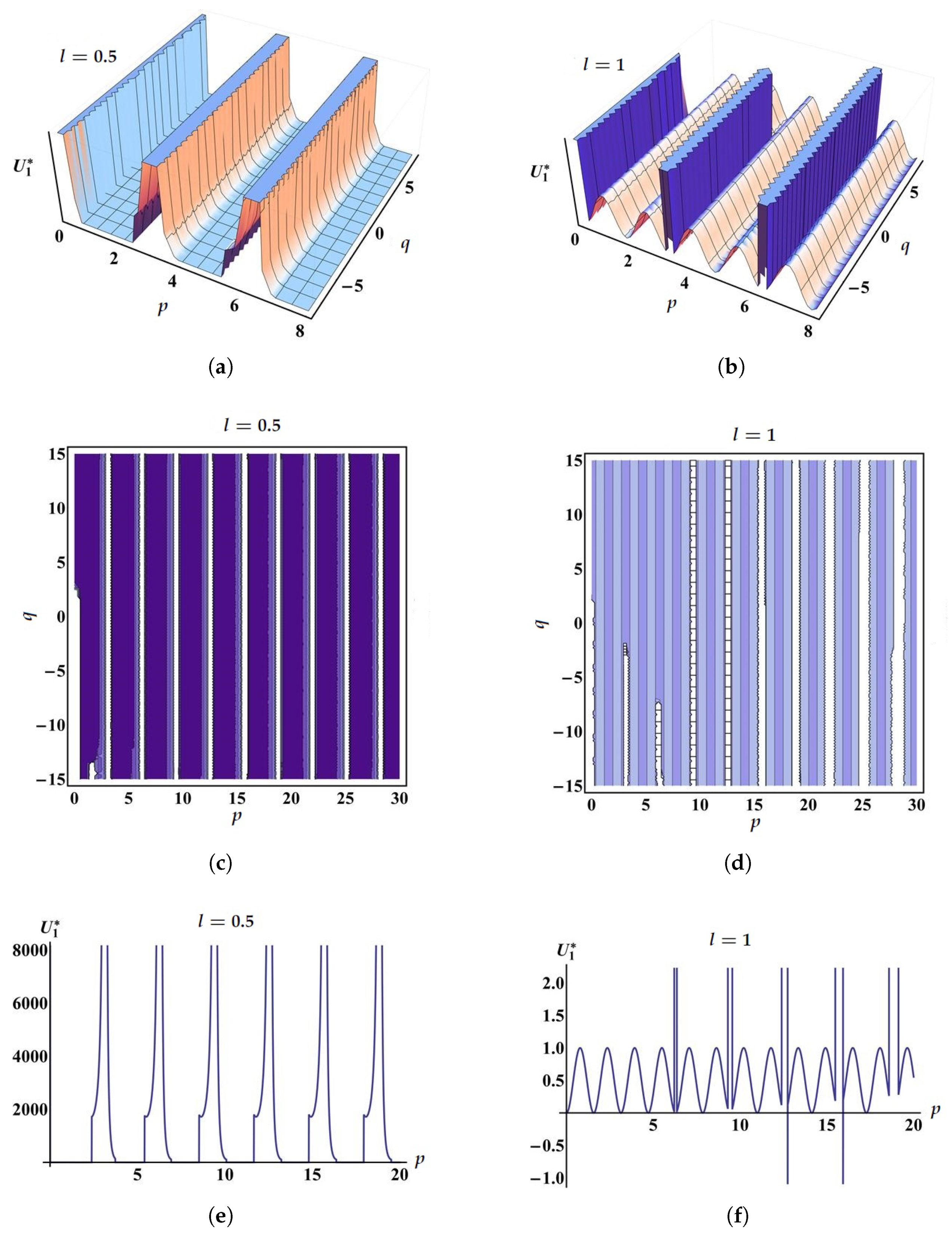
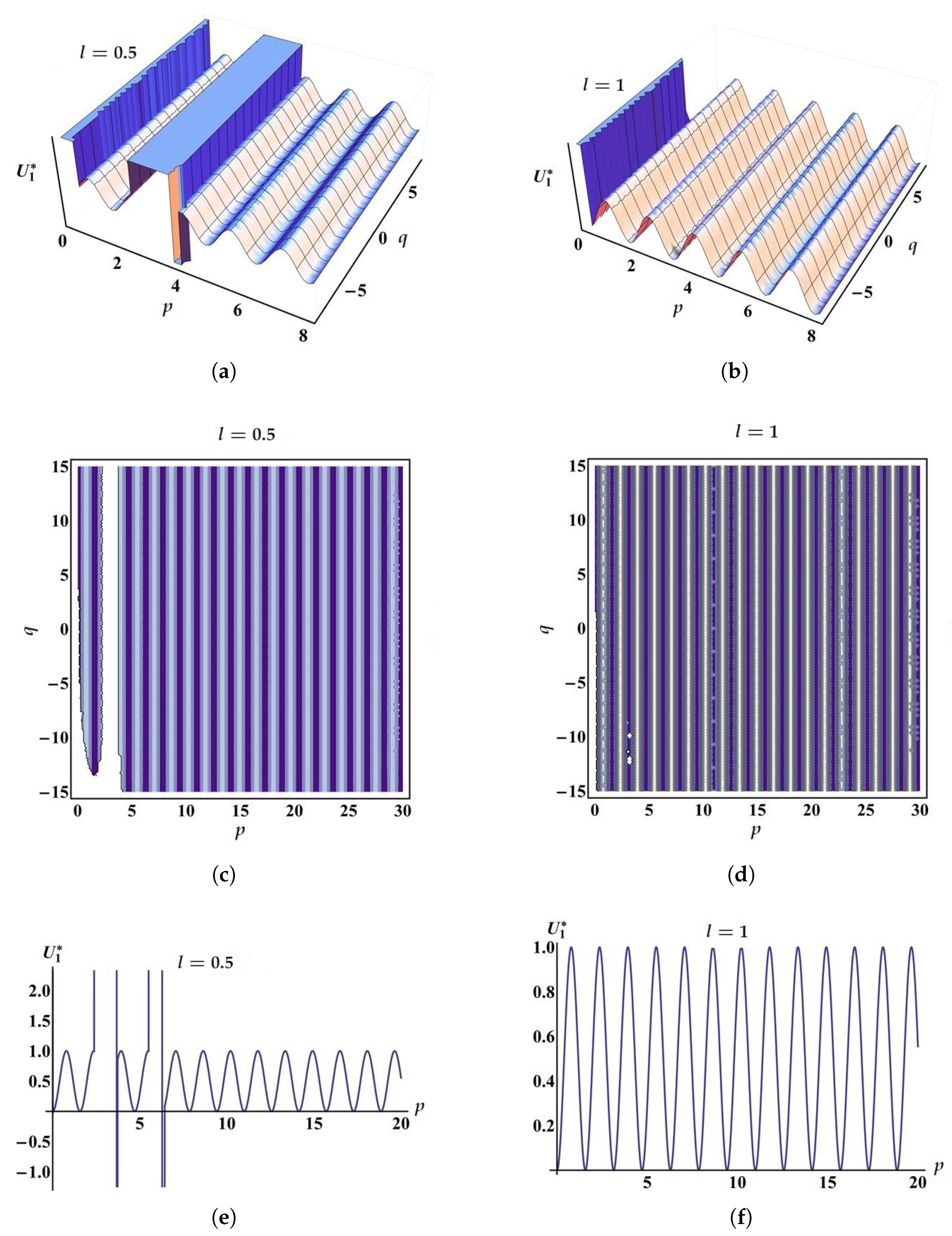
Remark 3.

The stochastic solutions (33)–(44) of Equation (14) strongly rely on the choosable functions $A_0\left(p\right),A_1\left(p\right),A_2\left(p\right),B_0\left(p\right),{\mathrm{\Lambda }}_1\left(p\right)$, and ${\mathrm{\Lambda }}_2\left(p\right)$. Hence, for various functions of this type, there exist different solutions of Equation (14), which can be extracted via Equations (33)–(44). In particular, this fact is shown for the solution $U_1.$ For the solutions $U_2,U_3,{\overline{U}}_1$, and ${\widehat{U}}_1,$ the procedures are analogous. Assume that $A_0\left(p\right)=A_0{B}_0^{\diamond 3}\left(p\right),{\mathrm{\Lambda }}_1\left(p\right)=A_1{B}_0\left(p\right),{\mathrm{\Lambda }}_2\left(p\right)=A_2{B}_0^{\diamond (-4)}\left(p\right),B_0\left(p\right)=\phi \left(p\right)+A_3{\vartheta }_1(p,l)\mathbb{L}\left(p\right),$ where $A_i(i=0,1,2,3)$ are arbitrary numbers, $\mathbb{L}\left(p\right)$ is the Gaussian one-variable white noise, which represents the time derivative of the Brownian motion $\mathbb{M}\left(p\right)$, and $\phi \left(p\right)$ is a real function, which is integrable in the sense of Definition 3. The Hermite transform of $\mathbb{L}\left(p\right)$ has the expansion $\stackrel{\sim }{\mathbb{L}}(p,z)={\sum }_{j=1}^{\infty }{z}_j{\int }_0^p{\psi }_j\left(\nu \right)d\nu$ [31]. By using the expansion of $\stackrel{\sim }{\mathbb{L}}\left(p\right)$, the identity ${exp}^{\diamond }\left(\mathbb{M}\left(p\right)\right)=exp\left(\mathbb{M}\left(p\right)-\frac{p^2}{2}\right)$ [31], and Equations (33)–(35), we acquire the following stochastic solution in a Brownian motion functional form:

$$U_1^{*}(p,q)=A_0{B}_0^2\left(p\right)-\frac{8{\kappa }^2{\left(l^{*}(p,q)\right)}^3[10A_2{B}_0^{-3}\left(p\right)+l^{*}(p,q)(A_1{B}_0\left(p\right)-3d{A}_2{B}_0^{-4}\left(p\right))]}{A_0{B}_0^2\left(p\right)},$$

(45)

where:

$$l^{*}(p,q)=\pm \sqrt{\frac{\eta }{Bexp\left(2\eta {\mathsf{\Omega }}^{*}(p,q)\right)+\kappa }},$$

(46)

and

$${\mathsf{\Omega }}^{*}(p,q)=-\frac{2d(A_0-d^2{A}_1+d^6{A}_0{A}_2)}{c}{\int }_0^p\frac{\phi \left(\nu \right)}{{\vartheta }_1(\nu ,l)}d\nu +{\int }_0^q\frac{d\nu }{{\vartheta }_2(\nu ,l)}+A_3\left(\mathbb{M}\left(p\right)-\frac{p^2}{2}\right).$$

(47)

Therefore, by picking adequate forms and values for the existent functions and parameters, we can represent the dynamical behavior of the obtained results. For $l=0.5$ and $1,$ the dynamical behavior of the wave solution (45) is explained by Figure 1 and Figure 2, when $A_0=A_3=0.5,A_1=-2.3,A_2=2.4,B=1,d=\eta =-c=2.5,\phi \left(p\right)=B_0\left(p\right)=sin\left(2p\right),{\vartheta }_1(p,l)=exp\left[(l-1)p\right]$, and ${\vartheta }_2(p,l)=exp\left[(1-l)p\right]$. Figure 1 elucidates the three-dimensional, contour, and two-dimensional dynamical behaviors of the wave solution (45) when the noise influence is absent $\left(\mathbb{M}\right(p)=0)$. Figure 2 demonstrates the three-dimensional, contour, and two-dimensional dynamical behaviors of the wave solution (45) under the noise influence $\mathbb{M}\left(p\right)=\mathrm{RAND}[0,1]\times exp\left(2p\right)$. From Figure 1 and Figure 2, it is deduced that the stochastic parts produce some disturbances in the amplitude of the traveling wave that represent the solution.

Moreover, from Figure 1 and Figure 2, one can realize that the total impact of the conformable factor l, which appears in the nonlinear terms of Equation (14), can provide a new comprehensive rate of change in the nonlinear dispersion of optical or other waves described by the Schrödinger–Hirota equation. In fact, applying the conformable factor in the nonlinear equation of motion causes the monotonicity of the nonlinear wave dispersion to increase or decrease. It is worth noting that, in Figure 1e,f, there are some strange nonlinearities that differ from what is familiar in nonlinear terms. These strange nonlinearities are due to the conformable differential operators proposed in Equation (14). These conformable operators generalize the classical ones and are physically interpreted as new velocities with directions depending on the conformable factor l. In fact, one can take the factor l with different numbers in $(0,1]$ and obtain different forms of the nonlinear wave dispersion. In our work, we only chose $l=0.5$ and $l=1$ as illustrative examples.

In the remaining portion of this section, we provide some comparative remarks that support our results.

Remark 4.

In [45], the authors used the helpful Equation (12) when $\sigma =2$ and $\kappa =\eta =1.$ In the current work, we employed this helpful equation when $\sigma =3$ and $\kappa ,\eta$ are arbitrary. Moreover, the present results were extracted in a stochastic conformable environment. This produces greater pluralism and realness in producing the exact solutions of the Schrödinger–Hirota equation.

Remark 5.

If we place the functions ${\vartheta }_1(p,l)={\vartheta }_2(p,l)=p^{1-l}$, then the gained solutions $U_1,U_2,U_3,{\overline{U}}_1$ and ${\widehat{U}}_1$ represent a novel group of wave solutions of the stochastic Schrödinger–Hirota equation with conformable operators proposed by Khalil et al. in [13]. Moreover, if $\kappa =\eta =B=1$ and $\sigma =2$, then the auxiliary Equation (12) reduces to:

$$\frac{dE}{dw}=E^2\left(w\right)-E\left(w\right),$$

(48)

and its solution becomes

$$E\left(w\right)=\frac{1}{1+exp\left(w\right)}.$$

(49)

Further, if we set $l=1$, $\mathbb{M}\left(p\right)=0$ and $\phi \left(p\right)={\phi }_0$ (constant), then ${\vartheta }_1(p,l)={\vartheta }_2(p,l)=1$, and all the conformable differential operators transfer to classical derivatives and all the stochastic coefficients reduce to deterministic ones. Hence, by simple calculations, one can see that all solutions of the Schrödinger–Hirota equation extracted in [4,46,47] can be obtained by our approach as spacial cases.

6. Conclusions

The Schrödinger–Hirota equation is one of the important nonlinear equations that describes the dynamics of soliton spread via optical fibers. In this work, we extracted a new group of deterministic and stochastic solutions of the Schrödinger–Hirota equation exactly in a Wick-type stochastic environment and with recent GDCOs. By combining the properties of GDCOs, some tools of white noise analysis, and the generalized Kudryashov scheme, a novel and direct methodology for constructing multiple solutions of the stochastic CNEEs with GDCOs was established. To highlight the usefulness and validity of this methodology, we applied it to construct diverse exact wave solutions of the Schrödinger–Hirota equation in a Wick-type stochastic space and with GDCOs. According to simple calculations, two significant types of wave solutions can be gained from our general exact solutions. These types of solutions are named soliton and periodic solutions and play considerable roles in many directions of nonlinear physical sciences. Moreover, a graphical visualization including three-dimensional, contour, and two-dimensional profiles was displayed for some of the gained solutions with the chosen functions and parameters. In Remarks 4 and 5, the significance of the resultant solutions was reinforced by some comparative aspects connected to some past research works on these types of solutions.

References

1. Ghanbari, B.; Nisar, K.S.; Aldhaifallah, M. Abundant solitary wave solutions to an extended nonlinear Schrödinger’s equation with conformable derivative using an efficient integration method. Adv. Differ. Equ. 2020, 2020, 328. [Google Scholar] [CrossRef]
2. Rezazadeh, H.; Abazari, R.; Khater, M.M.A.; Inc, M.; Baleanu, D. New optical solitons of conformable resonant nonlinear Schrödinger’s equation. Open Phys. 2020, 18, 761–769. [Google Scholar] [CrossRef]
3. Kumar, D.; Seadawy, A.R.; Joardar, A.K. Modified Kudryashov method via new exact solutions of some conformable fractional differential equations arising in mathematical biology. Chin. J. Phys. 2018, 56, 75–85. [Google Scholar] [CrossRef]
4. Rezazadeh, H.; Mirhosseini-Alizamini, S.M.; Eslami, M.; Rezazadeh, M.; Mirzazadeh, M.; Abbagari, S. New optical solitons of nonlinear conformable fractional Schrödinger–Hirota equation. Optik 2018, 172, 545–553. [Google Scholar] [CrossRef]
5. Soliman, A.H.; Hyder, A. Closed-form solutions of stochastic KdV equation with generalized conformable derivatives. Phys. Scr. 2020, 95, 065219. [Google Scholar] [CrossRef]
6. Zhao, D.; Luo, M. General conformable fractional derivative and its physical interpretation. Calcolo 2017, 54, 903–917. [Google Scholar] [CrossRef]
7. Alharbi, F.M.; Baleanu, D.; Ebaid, A. Physical properties of the projectile motion using the conformable derivative. Chin. J. Phys. 2019, 58, 18–28. [Google Scholar] [CrossRef]
8. Khaled, S.M.; El-Zahar, E.R.; Ebaid, A. Solution of Ambartsumian Delay Differential Equation with Conformable Derivative. Mathematics 2019, 7, 425. [Google Scholar] [CrossRef] [Green Version]
9. Zhao, D.; Pan, X.; Luo, M. A new framework for multivariate general conformable fractional calculus and potential applications. Physica A 2018, 510, 271–280. [Google Scholar] [CrossRef]
10. Choi, J.H.; Kim, H. Exact traveling wave solutions of the stochastic Wick-type fractional Caudrey-Dodd-Gibbon-Sawada-Kotera equation. AIMS Math. 2021, 6, 4053–4072. [Google Scholar] [CrossRef]
11. Korpinar, Z.; Inc, M.; Alshomrani, A.S.; Baleanu, D. The deterministic and stochastic solutions of the Schrödinger equation with time conformable derivative in birefrigent fibers. AIMS Math. 2020, 5, 2326–2345. [Google Scholar] [CrossRef]
12. Ulutas, E. Travelling wave and optical soliton solutions of the Wick-type stochastic NLSE with conformable derivatives. Chaos Solitons Fractals 2021, 148, 111052. [Google Scholar] [CrossRef]
13. Khalil, R.; Al Horani, M.; Yousef, A.; Sababheh, M. A new definition of fractional derivative. J. Comput. Appl. Math. 2014, 264, 65–70. [Google Scholar] [CrossRef]
14. Abdeljawad, T. On conformable fractional calculus. J. Comput. Appl. Math. 2015, 279, 57–66. [Google Scholar] [CrossRef]
15. Hyder, A.; Soliman, A.H. A new generalized θ-conformable calculus and its applications in mathematical physics. Phys. Scr. 2021, 96, 015208. [Google Scholar] [CrossRef]
16. Jarad, F.; Uğurlu, E.; Abdeljawad, T.; Baleanu, D. On a new class of fractional operators. Adv. Differ. Equ. 2017, 2017, 247. [Google Scholar] [CrossRef]
17. Khan, T.U.; Khan, M.A. Generalized conformable fractional operators. J. Comput. Appl. Math. 2019, 346, 378–389. [Google Scholar] [CrossRef]
18. Abdelhakim, A.A.; Machado, J.A.T. A critical analysis of the conformable derivative. Nonlinear Dyn. 2019, 95, 3063–3073. [Google Scholar] [CrossRef]
19. Atangana, A.; Khan, M.A. Validity of fractal derivative to capturing chaotic attractors. Chaos Solitons Fractals 2019, 126, 50–59. [Google Scholar] [CrossRef]
20. Kudryashov, N.A. One method for finding exact solutions of nonlinear differential equations. Commun. Nonlinear Sci. Numer. Simul. 2012, 17, 2248–2253. [Google Scholar] [CrossRef] [Green Version]
21. Ege, S.M.; Misirli, E. The modified Kudryashov method for solving some fractional-order nonlinear equations. Adv. Differ. Equ. 2014, 2014, 135. [Google Scholar] [CrossRef] [Green Version]
22. Kilicman, A.; Silambarasan, R. Modified Kudryashov method to solve generalized Kuramoto-Sivashinsky equation. Symmetry 2018, 10, 527. [Google Scholar] [CrossRef] [Green Version]
23. Gaber, A.A.; Aljohani, A.F.; Ebaid, A.; Tenreiro Machado, J. The generalized Kudryashov method for nonlinear space–time fractional partial differential equations of Burgers type. Nonlinear Dyn. 2019, 95, 361–368. [Google Scholar] [CrossRef]
24. Zayed, E.M.E.; Alurrfi, K.A.E. The modified Kudryashov method for solving some seventh order nonlinear PDEs in mathematical physics. World J. Model. Simul. 2015, 11, 308–319. [Google Scholar]
25. Salam, M.A.; Habiba, U. Application of the improved Kudryashov method to solve the fractional nonlinear partial differential equations. J. Appl. Math. Phys. 2019, 7, 912–920. [Google Scholar] [CrossRef] [Green Version]
26. Hyder, A.; Barakat, M.A. General improved Kudryashov method for exact solutions of nonlinear evolution equations in mathematical physics. Phys. Scr. 2020, 95, 045212. [Google Scholar] [CrossRef]
27. Arnous, A.H.; Ullah, M.Z.; Asma, M.; Moshokoa, S.P.; Zhou, Q.; Mirzazadeh, M.; Biswas, A.; Belic, M. Dark and singular dispersive optical solitons of Schrädinger-Hirota equation by modified simple equation method. Optik 2017, 136, 445–450. [Google Scholar] [CrossRef] [Green Version]
28. Biswas, A.; Jawad, A.J.M.; Manrakhan, W.N.; Sarma, A.K.; Khan, K.R. Optical solitons and complexitons of the Schrödinger–Hirota equation. Opt. Laser Technol. 2012, 44, 2265–2269. [Google Scholar] [CrossRef]
29. Kilic, B.; Inc, M. Optical solitons for the Schrödinger–Hirota equation with power law nonlinearity by the Bäcklund transformatioqn. Optik 2017, 138, 64–67. [Google Scholar] [CrossRef]
30. Biswas, A. Optical solitons: Quasi stationarity versus Lie transform. Opt. Quantum Electron. 2012, 35, 979–998. [Google Scholar] [CrossRef]
31. Holden, H.; Øsendal, B.; Ubøe, J.; Zhang, T. Stochastic Partial Differential Equations; Springer Science and Business Media, LLC: New York, NY, USA, 2010. [Google Scholar]
32. Braumann, C.A. Introduction to Stochastic Differential Equations with Applications to Modelling in Biology and Finance; Wiley: Hoboken, NJ, USA, 2019. [Google Scholar]
33. Egorov, V.; Maksimova, O.; Andreeva, I.; Koibuchi, H.; Hongo, S.; Nagahiro, S.; Ikai, T.; Nakayama, M.; Noro, S.; Uchimoto, T.; et al. Stochastic fluid dynamics simulations of the velocity distribution in protoplasmic streaming. Phys. Fluids 2014, 32, 121902. [Google Scholar] [CrossRef]
34. Zhang, Y.; Krasheninnikov, S. Novel approach to stochastic acceleration of electrons in colliding laser fields. Phys. Plasmas 2019, 26, 050702. [Google Scholar] [CrossRef] [Green Version]
35. Al Qarni, A.A.; Alshaery, A.A.; Bakodah, H.O. Optical solitons via the collective variable method for the Schrödinger–Hirota equation. Int. J. Appl. Comput. Math. 2021, 7, 8. [Google Scholar] [CrossRef]
36. Ray, S.S. Dispersive optical solitons of time-fractional Schrödinger–Hirota equation in nonlinear optical fibers. Physica A 2020, 537, 122619. [Google Scholar]
37. Savaissou, N.; Gambo, B.; Rezazadeh, H.; Bekir, A.; Doka, S.Y. Exact optical solitons to the perturbed nonlinear Schrödinger equation with dual-power law of nonlinearity. Opt. Quantum Electron. 2020, 52, 318. [Google Scholar] [CrossRef]
38. Melchert, O.; Demircan, A.; Yulin, A. Multi-frequency radiation of dissipative solitons in optical fiber cavities. Sci. Rep. 2020, 10, 8849. [Google Scholar] [CrossRef]
39. Sekha, G.A.; Kalikotay, P. Dynamics of self-reinforcing matter-wave in gravito-optical surface trap. Chaos 2019, 29, 103112. [Google Scholar] [CrossRef]
40. Seadawy, A.R.; Iqbal, M.; Lu, D. Propagation of kink and anti-kink wave solitons for the nonlinear damped modified Korteweg-de Vries equation arising in ion-acoustic wave in an unmagnetized collisional dusty plasma. Physica A 2020, 544, 123560. [Google Scholar] [CrossRef]
41. Wang, G.; Yang, K.; Gu, H.; Guan, F.; Kara, A.H. A (2+1)-dimensional sine-Gordon and sinh-Gordon equations with symmetries and kink wave solutions. Nucl. Phys. B 2020, 953, 114956. [Google Scholar]
42. Allen, J.E.; Frantzeskakis, D.J.; Karachalios, N.I.; Kevrekidis, P.G.; Koukouloyannis, V. Solitary and periodic waves in collisionless plasmas: The Adlam–Allen model revisited. Phys. Rev. E 2020, 102, 013209. [Google Scholar] [CrossRef]
43. Churilov, A.N. Orbital stability of periodic solutions of an impulsive system with a linear continuous-time part. AIMS Math. 2020, 5, 96–110. [Google Scholar] [CrossRef]
44. Vidal-Henriquez, E.; Zykov, V.; Bodenschatz, E.; Gholam, A. Convective instability and boundary driven oscillations in a reaction-diffusion-advection model. Chaos 2017, 27, 103110. [Google Scholar] [CrossRef] [PubMed] [Green Version]
45. Mirzazadeh, M.; Eslami, M.; Biswas, A. Dispersive optical solitons by Kudryashov’s method. Optik 2014, 125, 6874–6880. [Google Scholar] [CrossRef]
46. Eslami, M.; Rezazadeh, H.; Rezazadeh, M.; Mosavi, S.S. Exact solutions to the space-time fractional Schrödinger–Hirota equation and the space-time modified KDV-Zakharov-Kuznetsov equation. Opt. Quantum Electron. 2017, 49, 279. [Google Scholar] [CrossRef]
47. Kaur, L.; Wazwaz, A.M. Bright-dark optical solitons for Schrödinger–Hirota equation with variable coefficients. Optik 2019, 179, 479–484. [Google Scholar] [CrossRef]
Figure 1. When the noise influence is absent, (af) are three-dimensional (contour) (two-dimensional) profiles for the wave solution (45), when l = 0.5 and l = 1 , respectively.
Mathematics 09 02760 g001
Figure 2. Under the noise influence, (af) are three-dimensional (contour) (two-dimensional) profiles for the wave solution (45), when l = 0.5 and l = 1 , respectively.
Mathematics 09 02760 g002
Publisher’s Note: MDPI stays neutral with regard to jurisdictional claims in published maps and institutional affiliations.