Article

Spatial Pattern of Air Pollutant Concentrations and Their Relationship with Meteorological Parameters in Coastal Slum Settlements of Lagos, Southwestern Nigeria

by
Oluwaseun Princess Okimiji
1,2,
Kuaanan Techato
1,
John Nyandansobi Simon
1,
Opeyemi Oluwaseun Tope-Ajayi
2,
Angela Tochukwu Okafor
3,
Moses Akintayo Aborisade
4 and
Khamphe Phoungthong
1,*
1
Environmental Assessment and Technology for Hazardous Waste Management Research Center, Faculty of Environmental Management, Prince of Songkla University, Hat Yai 90110, Songkhla, Thailand
2
Department of Environmental Management and Toxicology, Federal University of Agriculture, Abeokuta P.M.B 2240, Ogun State, Nigeria
3
Department of Environmental Management and Toxicology, Michael Okpara University of Agriculture, Umudike P.M.B 7267, Abia State, Nigeria
4
School of Environmental Science and Engineering, Tianjin University, Tianjin 300350, China
*
Author to whom correspondence should be addressed.
Atmosphere 2021, 12(11), 1426; https://doi.org/10.3390/atmos12111426
Submission received: 4 October 2021 / Revised: 27 October 2021 / Accepted: 27 October 2021 / Published: 29 October 2021
(This article belongs to the Special Issue Air Pollution, Air Quality and Human Health)

Abstract

:
This study assessed the spatial disposition of air pollutants and their relationship with meteorological parameters in urban slum settlements of Lagos city. The gaseous pollutants were quantified using a gas analyzer, and the PM2.5 concentration and meteorological parameters were determined using an Air Metric Sampler and Wind Mate, respectively. SPSS for Windows and ArcGIS were used for data analysis. The results revealed that the seasonal variations in SO2, NO2, CO2, and PM2.5 showed a higher level of air pollutant concentration during the dry season than during the wet season. During the wet season, a significant correlation was observed between PM2.5 and temperature at the 1% level (0.957 **), and VOC and SO2 (0.907 *) at the 5% level; during the dry season, significant correlations were observed between NO2 and SO2 at the 1% level (0.9477 **), and PM2.5 and relative humidity (0.832 *) at the 5% level. Atmospheric pressure (72%), temperature (60%), and relative humidity (98.4) were the primary meteorological factors affecting air pollutants such as VOC, CO2, and SO2. The spatial dispersal of air pollutants revealed a high Z score and a moderate p-value, indicating hot spot locations throughout the five selected slum settlements. It is recommended that regular monitoring based on quantifiable economic costs that are beneficial to the well-being of the populace be investigated, and policy-based initiatives for air pollution control based on scientific evidence be advocated for.

1. Introduction

Environmental problems such as air pollution are the direct consequences of an opaque population [1]. Hence, a substantial problem with air pollution is seen mostly in underdeveloped countries [2]. Consequently, underdeveloped countries are increasingly contending with rampant urban sprawl, commerce evolution, traffic emissions, and increasing urban populations [3,4]. Developing cities are subject to population explosions, degrading environmental quality, and increased costs of urban services. The internal growth of cities and migration to urban centers exceed by far the creation of jobs [5]. In a recent study, it was projected that more than 60% of Nigerians will live in urban centers by 2025, and a considerable proportion will likely live in slums if action is not taken [6].
Slum conditions are a significant issue in sub-Saharan Africa, and the slum situation in Nigeria is already problematic because of the proportion of people affected. The official figure is 42 slum areas, according to the UNDP and World Bank [7]. Researchers have estimated the population of slum dwellers in Lagos to be at 60–70% [8]. Accordingly, [9] documented the communities of Majidun, Amukoko, Agege, Ijora-Badia, Bariga, Iwaya, and Makoko as the largest slum settlements in Lagos, as classified by the World Bank. The authors of [10] ascertained that Nigeria’s inability to strategize and control fast-growing urban centers has resulted in overpopulation, leading to air pollution in the entire urban center of Lagos.
The air pollution in Lagos originates from both anthropogenic and natural factors [11]. However, particular aerodynamic diameters released during the burning of biomass fuel and traffic emissions are the most significant challenge to underdeveloped nations, especially Nigeria [12]. Lagos showed elevated levels of particles caused by smog events in the city on the 12th of October 2005 [13]. These air pollutants were of anthropogenic and biogenic origin, and thus could originate from stationary pollution, chemical and vehicular exhaust emissions [14], smoke from tobacco, chemicals for cleaning, the use of solvents, the incineration of solid waste, the evaporation of gasoline, gas, and petroleum leakage [15]. Air pollutant accumulation caused by anthropogenic activities such as traffic emissions and industrial activity has resulted in worsening air pollution-related issues [16].
Air pollutant concentrations rely on direct emissions and the quantity of gaseous precursors, which are NO2, SO2, CO2, and PM2.5, as well as meteorological variables [17]. Meteorological conditions affect the dispersion of air pollutants [18], and also control atmospheric pollution on a moderately abrupt continuance scale [17]. Multiple factors, such as pollutant transportation and transformation, pollutant emissions, and meteorological conditions, affect air pollution [19,20]. Studies have uncovered that both meteorological conditions and air pollutant emissions dominate pollutant concentration trends [21,22]. The authors of [23] reported that favorable meteorological conditions have important effects on air criteria, by impacting dispersal conditions and thus the environmental capacity. Hence, both regional and local meteorology have an effect on the temporal and spatial ordering of air pollutants [22]. The authors of [24] ascertained that more than 70% of the daily air pollutant absorption in China could be attributed to meteorological conditions. The authors of [25] documented that there is no clear linear relationship between the air pollutant concentration due to chemical transformation and meteorological parameters such as relative humidity, temperature, and atmospheric pressure. For instance, an increase in clouds can cause an increase in sulfates and nitrates due increased sulfate heterogeneous reactions in water [26].
Several studies have also assessed the effectiveness of adopted measures, pollution reduction, and forecasting air quality [27,28,29,30]. The authors of [31] carried out monitoring and intensity analysis of slum growth in Lagos. The authors of [32] carried out a study on slum upgrading in the era of world-class city construction, while [33] assessed the social capital and higher resilience of slums in the Lagos metropolis. The authors of [34] worked on the spatiotemporal urban growth dynamics of the Lagos Metropolitan region of Nigeria based on hybrid methods for LULC modeling and prediction, but there was no unified, high-resolution, and time-varied air pollutant emission information for the 42 identified communities in Lagos, which were ranked based on their level of decay [35]. In recent years, studies have developed statistical/empirical models, especially for Lagos slum settlements, but only a few have been able to predict air pollutant concentrations arising from meteorological inputs. Researchers [36,37,38,39] have been able to explore the relationship between air quality dynamics and meteorology parameters in Dhaka city to a large extent. Most importantly, multiple non-linear regression models have been applied to explore the significance and role of various meteorology parameters, such as relative humidity, temperature, atmospheric pressure, and precipitation, on particulate and gaseous air pollutants [39]. Bivariate Pearson correlation coefficients were also employed to determine the relationship between meteorological parameters and air pollutants [37]. Additionally, the cross-correlation approach and multi-linear regression were also used to assess the effect of meteorological variables on seasonal changes in particulate matter disposition in Dhaka city [38]. Several studies have considered the source apportionment [40,41], elemental characterization [42,43], and spatiotemporal distribution [42] of particulate matter in Dhaka city.
However, there remains a knowledge gap between meteorological parameters and their impacts on concentrations of air pollutants. In this study, a systematic analysis, comprising the cross-correlation approach, multi-linear regression, and kriging and Getis–Ord general G statistics interpolation method, was used to investigate the relationships between air pollutants (PM2.5, CO2, SO2, NO2, and VOC) and meteorological parameters (temperature, atmospheric pressure, and relative humidity) in five selected slum settlements, based on a 12-month record of observations from 2018 to 2019. The goal was to understand these vital relationships in order to improve the understanding of the mechanisms that produce air pollution, enhance the forecast accuracy of air pollution, and provide effective measures for mitigating pollution. The objective of this study was to discuss the variation in air pollutant concentrations in coastal slum settlements, driven by meteorological parameters and the emissions of their precursors. The discussion includes: (i) the spatial pattern of air pollutant concentrations, (ii) meteorological factors that affect air pollutant concentrations and their relationship with meteorological variables, and (iii) the influence of meteorological parameters on ambient air quality in coastal slum settlements. This study will provide the necessary reference information for local governments to develop atmospheric environment pollution control strategies, and an emergency plan for coastal slum dwellers. Moreover, we evaluated the spatial pattern of the air pollutant concentration; unlike in most developed societies, where air quality monitoring is carried out routinely, environmental researchers undertake air quality assessments in most countries of sub-Saharan African, including Nigeria. Nevertheless, environmental agencies, city administrators, and residents need this information to safeguard the wellbeing of the people. Among the citizenry, this information will possibly motivate communal action to demand proper attention through responsible leadership.

2. Materials and Methods

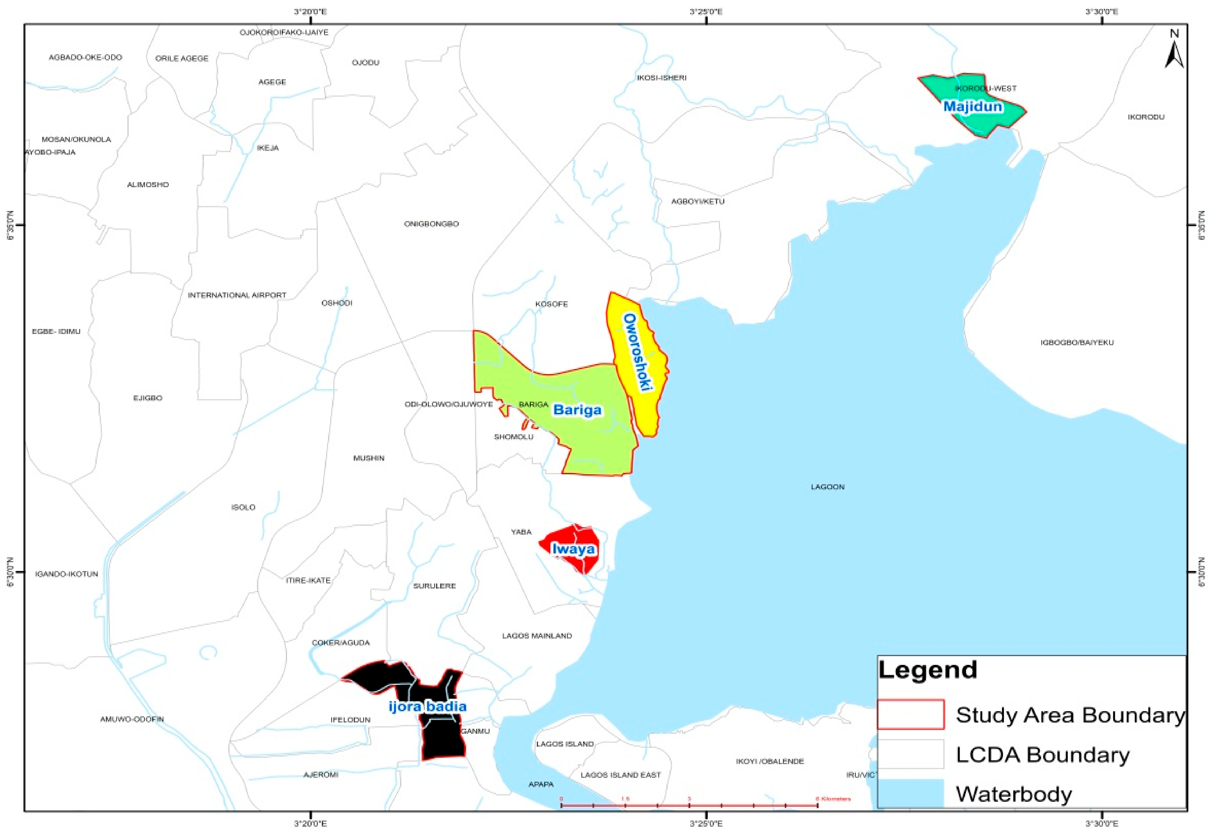
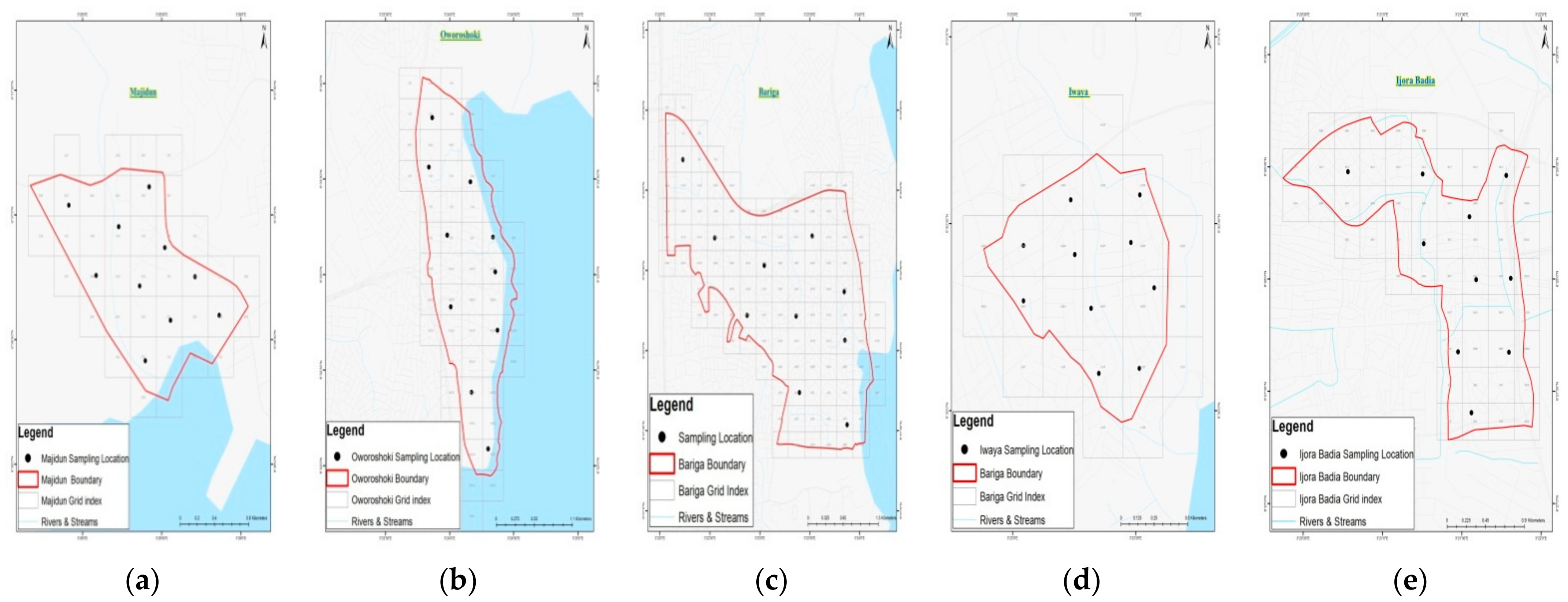
2.1. Study Area and Sample Site

The study area was the coastal slum settlement geomorphological unit of the Lagos metropolis, Southwestern Nigeria, which lies roughly between latitudes 6°30′ N and 6°40′ N and longitudes 3°00′ E and 4°00′ E. The study area occupies approximately 1171.28 km2 of land, covering luculent geographical settlements, with a population density of 6871 residents per square kilometer [44]. Its climate is characterized by two major vegetation types/climates, freshwater swamp and wet lowland tropical rainforest climates, with two distinct climatic seasons (a dry and a wet season) [45]. The region is drained by a dendritic drainage system comprising rivers that flow into the Lagos Lagoon, which ultimately discharges into the Atlantic Ocean [46]. In terms of population size, Lagos State is estimated to have a population ranging from 24.5 million in 2015 to 29 million by 2025 [10]. The population growth rate is estimated to range between 2.35% [7] and 8.0% [47], which represents a 3.44% annual change [48]. The authors of [49] identified 42 communities in Lagos and ranked them based on their level of decay [35]. Five of these communities were selected for this study: the Ijora-Badia, Iwaya, Majidun, Oworoshoki, and Bariga slums (Figure 1).

2.1.1. Ijora-Badia

The Ijora-Badia slum is one of the earlier identified slums (1984) and is located in Lagos Island, in the Apapa local government area, with an estimated population of 217,661 [44]. The settlement consists of three sub-communities: Oke Ilu-eri, Ajeromi, and Railway Line [33]. It is bordered on the north by the Lagos Badagry Expressway, on the east by a railway line running parallel with the Apapa road, and on the south by Ajegunle (another slum community) [33]. The earliest settlers of Ijora-Badia were displaced from the present-day location of the Nigeria National Art Theatre, Iganmu Lagos, after the federal government acquired the land through forceful eviction, without adequate consultation or compensation, in order to build the theater [50].

2.1.2. Iwaya

The Iwaya slum is located in mainland Lagos’ local government area. The community shares a boundary with another slum community [51]. The population is the smallest among the slum settlements, and the slum is enclosed by land. The estimated population was 58,000 and 725 persons per hectare in the 1995 projection [7]. It has close proximity to the University of Lagos, which aids its continuous growth. The community encroaches on water bodies, which can be seen from the Lagos third mainland bridge. Various ethnic groups live in Iwaya but are separated into sub-communities, such as Pedro/Shogunro, Ago Egun, and Iwaya Central. The community comprises both poor people [52] and white-collar workers [53]. Most of the residents engage in carpentry, fishing, and trading. The Iwaya slum has experienced forceful eviction of its residents and several demolition exercises. The Lagos State Government demolished more than 200 houses in August 2017 [54].

2.1.3. Majidun

Majidun is located in the Ikorodu local government area of Lagos State, in a peri-urban area, and had an estimated population of 40,195 and a population density of 638 persons per hectare in the 1995 projection [7]. The Yoruba ethnic group is the dominant group, and most of the buildings in these slums are referred to as family compounds rather than a slum community, as stated by the ruler of the area (king of Ikorodu community). Most of the houses are of mud type, and the community still shows the features of a traditional Yoruba town. The occupations of the residents include trading, tailoring, barbing, and pottery [55].

2.1.4. Oworoshoki

The Oworoshoki slum is located in the Somolu local government area of Lagos State. The estimated population is approximately 402,673 [56] in a land area of 11.6 km2. According to Adeniyi et al. [57], the Oworoshoki community shares a boundary with the Bariga Local Government area in the north, while, in the south, it shares a boundary with the Akoka community. In the east, the boundary is the major Ikorodu road from Fadeyi to Anthony, and in the west, it is Abule-Ijesha. The community is surrounded by swamp vegetation, located further north of its boundary in the Kosofe local government area [57].

2.1.5. Bariga

Bariga is located in the Kosofe local government area of Lagos State. It is located in the northern part of the state and bounded by three local governments: Ikeja, Ikorodu, and Shomolu [58]. Its estimated population is 682,772 in an area of 178.85 km2 [56]. Bariga vegetation is mostly swamp forest, encroached on by buildings and marketplaces. The indigenous dwellers are mainly the “Aworis”, whose major occupations are trading, mat-weaving, and fishing. A map of the Lagos metropolis was obtained and gridded to create cells of 300 m2 using Arc Map 10.1, as shown in Figure 1. Ten cells were randomly selected from each of the study areas using a random number table, according to the kriging method [59].

2.2. Measurement and Sampling of Pollutants

Ambient air and meteorological sampling were carried out at the five selected coastal slum settlements in the Lagos metropolis: Slum A (Ijora-Badia); B (Bariga); C (Majidun); D (Iwaya); and E (Oworoshoki). At each slum settlement, the air pollutant parameters were carbon dioxide (CO2), sulfur dioxide (SO2), nitrogen dioxide (NO2), volatile organic compounds (VOCs), and particulate matter (PM2.5). The meteorological parameters were temperature, relative humidity, and atmospheric pressure. These were measured four times per month for six months (June, July, August, September, October, November) in the wet season and six months (December, January, February, March, April, May) in the dry season from June 2018 to May 2019. In totality, 12 months of air pollution and meteorological monitoring were carried out across the sample locations. The geographical coordinates (latitude-x coordinate and longitude-y coordinate) of the sample sites were determined using a GPS device from Garmin (GPSMAP 76CSX model). A handheld portable gas analyzer (multi-RAE PGM-6208) was used for CO2, SO2, NO2, and VOC measurement in the windward direction at the sample locations. An Air Metric Sampler (PDR.1000AN) measuring kit was used on-site for measuring PM2.5 data. A Wind Mate (WM 350) instrument was used for measuring the meteorological parameters. All the measurements were taken at a time-weighted average with a digital meter, at 2 m from ground level, where humans are most likely to be exposed. This procedure was repeated for accuracy and reliability, and the monitoring dimensions were taken in triplicate. According to the manufacturer’s recommendation, the equipment was calibrated before and after each batch of samples.
The measurement techniques used for monitoring the reported criteria pollutants in this study were carried out according to the method proposed by [60,61]. The instruments used in the experiments provide an industry-leading array of interchangeable field-replaceable electrochemical, combustible, infrared, photoionization detector (PID), and gamma radiation sensors for a wide variety of applications. The instruments are digital meters that take time-weighted average measurements. The uncertainty associated with the instruments is primarily due to the devices not being calibrated before use, which results in inaccurate readout data. Additionally, not zeroing, erasing, or resetting the current data after use may affect the readout readings during the following sampling period. The hand-held portable gas analyzer (multi-RAE PGM-6208) was calibrated utilizing the “Two-point field calibration for zero and standard reference gases” method (span gas). VOC detection limits range from 100 to 2,000,000 mg/m3; SO2 detection limits range from 100 to 20,000 mg/m3; NO2 detection limits range from 100 to 20,000 mg/m3; and CO2 detection limits range from 1000 to 500,000 mg/m3. Calibration of the Air Metric Sampler (PDR.1000AN) for the measurement of PM2.5 was performed using two collectors of reference filters and two master real-time monitors (Thermo Electron Data RAM 4), with a detection limit of 1–4.0 × 10⁵ µg/m3. The Wind Mate (WM 350) device that was used to measure meteorological parameters had been pre-calibrated according to the manufacturer’s specifications.

2.3. Air Pollutant Data and Quality Assurance

Ambient air and meteorological sampling was carried out in situ using various calibrated hand-held devices. Air pollutant and meteorological parameter monitoring was carried out in one-hour triplicate periods three times per day (morning, afternoon, and night), based on limits set by USEPA [62] and FMEnv [63]. The hourly ambient air pollutant concentration was collected using different equipment calibrated according to the manufacturer’s recommendations for the gaseous, particulate, and meteorological parameters. These measurements were carried out at 50 points for each sample location, and replicated three times. Accordingly, data were generated based on the equipment’s standards and methods. Beforehand, screening of the raw data was conducted to ensure the accuracy of the obtained air pollutant and meteorological data. Missing data and maximal or minimal data for abrupt growth were removed. Hourly data were then used to generate the daily mean using at least 20 h of valid data. Secondly, monthly means were derived from the daily mean data, and an overall 20 days of valid data were used. The data were then used to generate the seasonal mean. Thirdly, validated data for the sample year were used to calculate the relationship and influence of these pollutant parameters.
Missing data showed the same pattern across the five selected sample sites. The air pollutant concentrations across the air sampling sites in each slum settlement were calculated as the air pollutant concentration at the coastal slum community level. Several baselines of 1 h and 24 h mean concentrations proposed based on the NAAQS [64], WHO [65], and FMEnv [63] were adopted for this study.

2.4. Assessment of Spatiotemporal Variations of Air Pollutants

The spatial data for this study included the duration of sampling, categorizing released pollutants, air pollutant concentrations, and geographical locations, for a representative collection of data across all the slum settlements. Air pollutant data from ground observations were imported into digital map layers for spatial analysis of the Lagos metropolis. Location coordinates were saved in Excel, and the shapefile representing the current scope of the Lagos metropolis was sourced into the GIS platform using ArcGIS 10.0 software. After assigning attribute data to spatial objects, the system was ready for spatiotemporal analysis and operation. Mapping of the areas with different concentration levels was carried out using the kriging and Getis–Ord general G statistics interpolation method in the ArcGIS 10.0 environment. The spatial analysis employed in this study used hot spot analysis, where vectors were used to identify the major hot spot and cold spot areas. In this way, density was considered in this study, suggesting where clusters existed in the dataset, while points were used to add up to polygons [66]. Getis–Ord general G statistics were used for this study, which gave the Z scores and p-values. A high Z score and a modest p-value implied a significant hot spot location. A negative Z score and a low p-value suggested the presence of a substantial cold spot. A higher Z score implied more intense clustering, while an A–Z near zero score meant no spatial clustering [67].
The Getis–Ord statistic is given as:
      G i * = j = 1   n w i , j x j X   j = 1   n w i ,   j [ n   j = 1 n w 2 s i , j j = 1 n w i ,   j
where xj is the criterion value for feature j, wi, j is the spatial weight between features i and j, and n is the total number of features and:
X = j = 1 n x j n  
s = j = 1 n X 2 j n X 2  
The kriging and Getis–Ord general G statistics interpolation method was used to predict the movement of air pollutant parameters from slum A to other slum locations within the Lagos metropolis. The obtained readings for the distribution map development were computed into ArcGIS 10 software to pre-define ranges of the respective air quality parameters. Maps were produced as colored gradients, representing the distribution pattern of the respective ranges of the parameters. Figure 2 presents the spatial gradient maps of the five selected coastal slum settlements in the Lagos metropolis.

2.5. Statistical Analysis

The statistical analysis employed in this study included descriptive and inferential statistics (SPSS windows, version 21.0). The trend in air pollutant concentrations was plotted on a line graph; the level of association between air pollutants and meteorological parameters was determined using correlation analysis. Multivariate regression analysis was used to assess the influence of the meteorological parameters on the air pollutant concentrations. In order to identify the factors that could explain the variation in the levels of sampled air quality parameters, the meteorological parameters of relative humidity (RH), temperature (T), and atmospheric pressure (AP) served as the explanatory variables (X), and the concentrations of selected air quality parameters were the dependent variable (Y); this is shown in Equation (4). The predictor variables were screened for multi-collinearity using inter-correlation analysis, so as to ensure accurate values for each in the regression models. All three variables had r2 values above 60.7%, so were suitable for the analysis [68].
Y = a + b 1 × 1 + b 2 × 2 + b 3 × 3 + e
where:
Y = value for the dependent variable (air quality parameters);
b = the quotients of the predictor variable (parameter X);
a = the intercept of model slope;
x = value of the independent variable;
e = estimation error.

3. Results

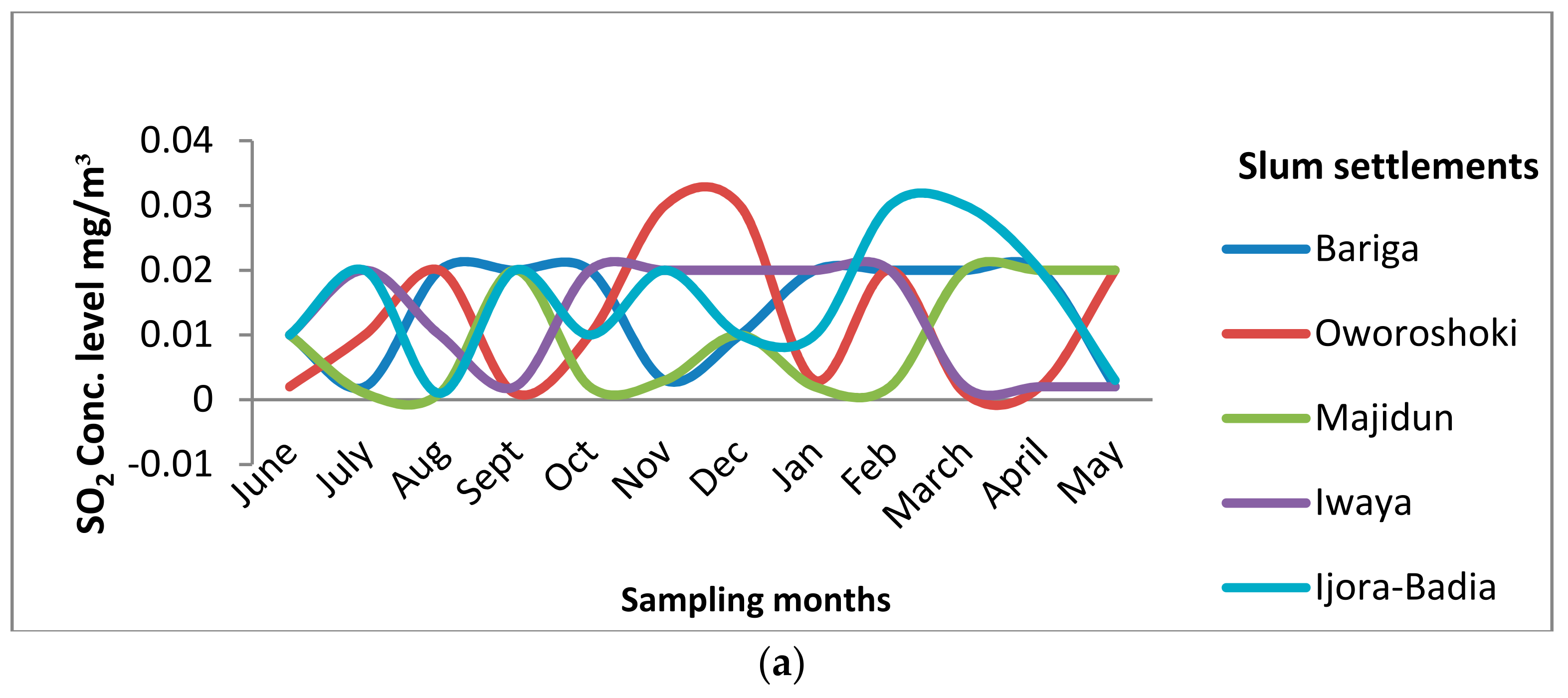
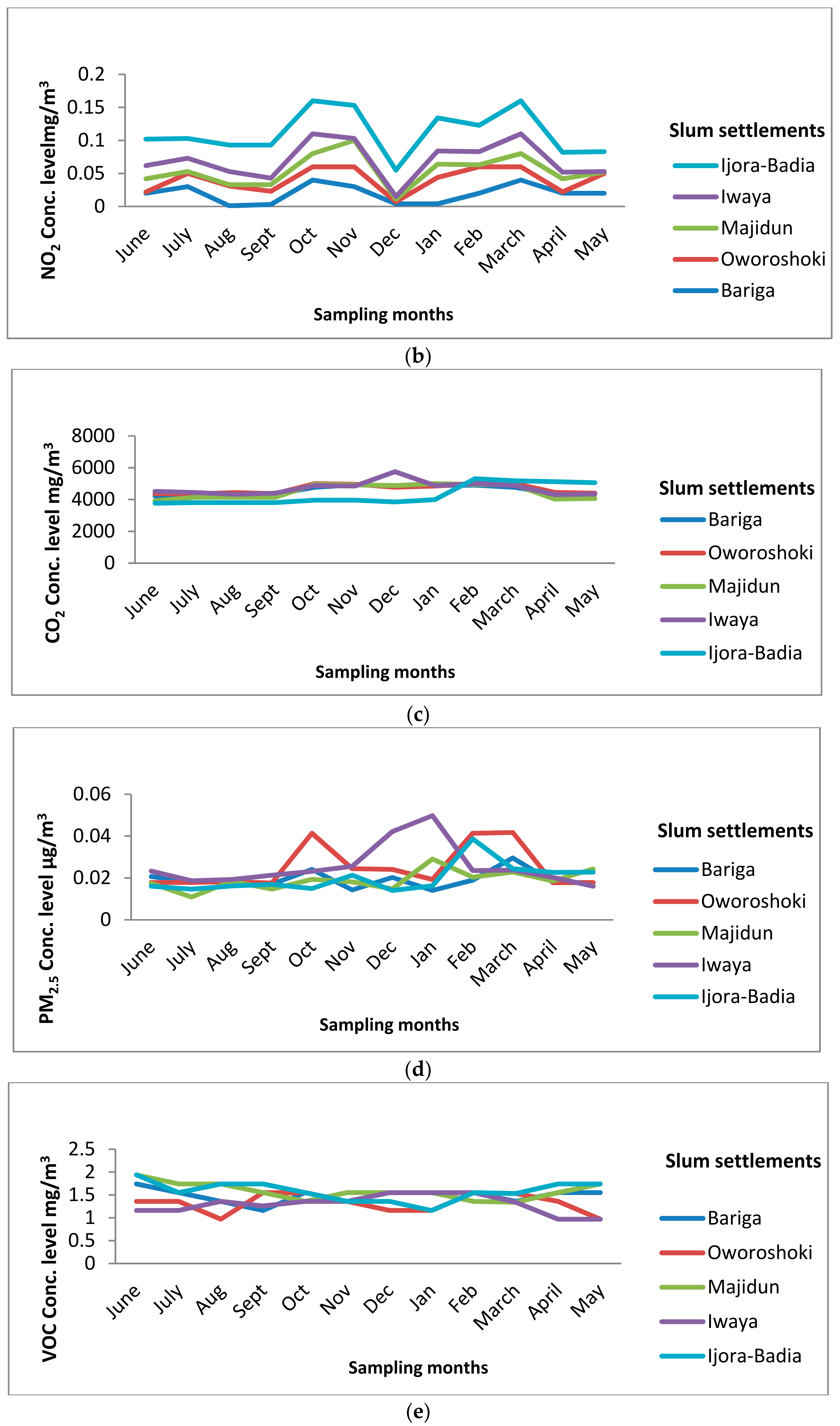
3.1. Seasonal Variation in Air Pollutants

The variation in air pollutants monitored from June 2018 to May 2019 revealed the trend patterns of the pollutants in five selected coastal slum settlements (Figure 3a–e). Based on the available data, the observed variation in all air pollutants was 0.001–0.03 mg/m3 (SO2), 0.001–0.05 mg/m3 (NO2), 3770–5750 mg/m3 (CO2), 1.09–4.97 µg/m3 (PM2.5), and 0.96–1.94 mg/m3 (VOC). It can be seen that from 2018 to 2019 (Figure 3a–e), there was an incremental change in the concentration level of air pollutants at the peak for SO2, NO2, CO2, PM2.5, and VOC (0.02–0.03 mg/m3, 0.03–0.04 mg/m3, 4510–5750 mg/m3, 3.86–4.97 µg/m3, and 1.74–1.94 mg/m3, respectively). There were significant reductions observed at the troughs for these air pollutants, in the range of 0.001–0.01 mg/m3, 0.001–0.02 mg/m3, 3770–4400 mg/m3, 1.09–2.90 µg/m3, and 0.96–1.55 mg/m3 for SO2, NO2, CO2, PM2.5, and VOC, respectively. According to the variations in the trend analysis, ambient air pollution of SO2 (October, November, December, January, and February), NO2 (September, October, November, and January), CO2 (November, December, and January), and PM2.5 (October and December) showed a higher concentration during the dry season. There were slight increments observed in the wet season for the months of March, April, and May (SO2), March and April (NO2), February and March (PM2.5), and June and July (VOC). In line with the observations from this study, Oworoshoki and Ijora-Badia showed a strong pattern for the SO2 concentration, while Ijora-Badia, Oworoshoki, Bariga, Majidun, and Iwaya showed a notable concentration pattern for NO2 pollution. Moreso and Iwaya experienced huge CO2 pollution. Oworoshoki, Iwaya, and Ijora-Badia had higher magnitudes of PM2.5 pollutants, while Majidun and Ijora-Badia experienced enormous VOC pollution.

3.2. Temporal Variations in Air Pollutant Concentrations in the Slum Settlements

The seasonal variation of the CO2 concentration is presented in Table 1. In the wet season, the mean concentration of CO2 was between 3843 and 4400 mg/m3, while in the dry season, it was 4874 to 5208 mg/m3 across all of the slum settlements. The obtained values were within the recommended threshold value of carbon dioxide in the environment.
The level of SO2 recorded in this study ranged from 0.005 to 0.015 mg/m3 in the wet season and between 0.009 and 0.026 mg/m3 in the dry season (Table 1). This exceeded the WHO [65] limits of 0.2 mg/m3 for daily average limits, while some of the study areas recorded values within the recommended limits. The obtained values were well below the NAAQS [64] (1 h) recommended limit of 0.075 mg/m3. Thus, the annual standard for SO2 is 3.0 mg/m3 [62].
The level of PM2.5 in the study area ranged between 1.734 and 1.956 µg/m3 in the wet season and 1.876 and 3.348 µg/m3 in the dry season (Table 1). The obtained values were within the suggested limits for an hour, but when multiplied by 24 h, the resultant value surpassed the WHO [65], NAAQS [64], and FMEnv [63] limits of 25 ug/m3 for 24 h. The NO2 level in this study varied from 0.014 to 0.024 mg/m3 in the wet season and 0.005 to 0.044 mg/m3 during the dry season (Table 1). The results obtained in some of the study regions were within the NAAQS [64] limit of 0.1 mg/m3 (1 h) and 0.05 mg/m3 (24 h), whereas values in other places surpassed the NAAQS [64] limit of 0.1 mg/m3 (1 h).
The volatile organic compounds level ranged between 1.192 and 1.898 mg/m3 (wet season) and 1.346 and 1.466 mg/m3 (dry season). The obtained values were within the NAAQS [64] limit of 6000 mg/m3 for 24 h, while some of the study areas obtained values exceeding the WHO [65] limit of 0.02 (1 h) mg/m3.

3.3. Relationship between Air Quality and Meteorological Parameters

The result of the correlation analysis for the five selected slum settlements in the wet seasons is shown in Table 2. A strong negative correlation was found between VOC and CO2 (r = −0.937 **), VOC and PM2.5 (r = −0.874 **), CO2 and SO2 (r = −0.994 **), NO2 and PM2.5 (r = −0.925 *), and SO2 and temperature (r = −0.835 *) across the study areas during the wet season. This implies that an increment in one parameter leads to a decrease in other parameters.
A positive correlation existed between VOC and SO2 (r = 0.907 *) and PM2.5 and temperature (r = 0.937 **). A decrease in one parameter will lead to a decrease in another parameter (Table 2).
Based on the information given in Table 3, the results showed a strong positive correlation between NO2 and SO2 (r = 0.947 **) and PM2.5 and relative humidity (r = 0.832 *). The strong association between PM2.5 and relative humidity can be explained by the presence of very humid aerosols, which create a positive artifact. There was a strong positive correlation between NO2 and SO2 and PM2.5 and temperature, meaning that an increase in one parameter will lead to an increase in another parameter.

3.4. Influence of Meteorological Parameters on Air Pollutants

The influence of temperature, relative humidity, and atmospheric pressure was evaluated for both the wet and dry seasons using linear regression analysis. The results, shown in Table 4, revealed that relative humidity had a strong coefficient of determination with VOC of r2 = 92.6%, NO2 of r2 = 78.3%, and SO2 of r2 = 89.2%. A strong coefficient of determination was also observed for temperature with CO2 of r2 = 99.7% and PM2.5 of r2 = 100%. Atmospheric pressure had a strong positive coefficient of determination with PM2.5 at r2 = 100% during the wet season. Significant and non-significant coefficient relationships were observed among the meteorological and air pollutant parameters.
As seen in Table 5, atmospheric pressure was positively correlated with all the air pollutant parameters in the dry season. The coefficient of determination for VOC was r2 = 72.0%, CO2 was r2 = 73.8%, SO2 was r2 = 84.4%, and PM2.5 was r2 = 98.4%. A moderate coefficient of determination also existed between atmospheric pressure and NO2 of r2 = 60.7%. Relative humidity was found to possess a positive coefficient of determination with PM2.5 of r2 = 100%. There were statistically significant coefficients of determination among the meteorological and air pollutant variables.

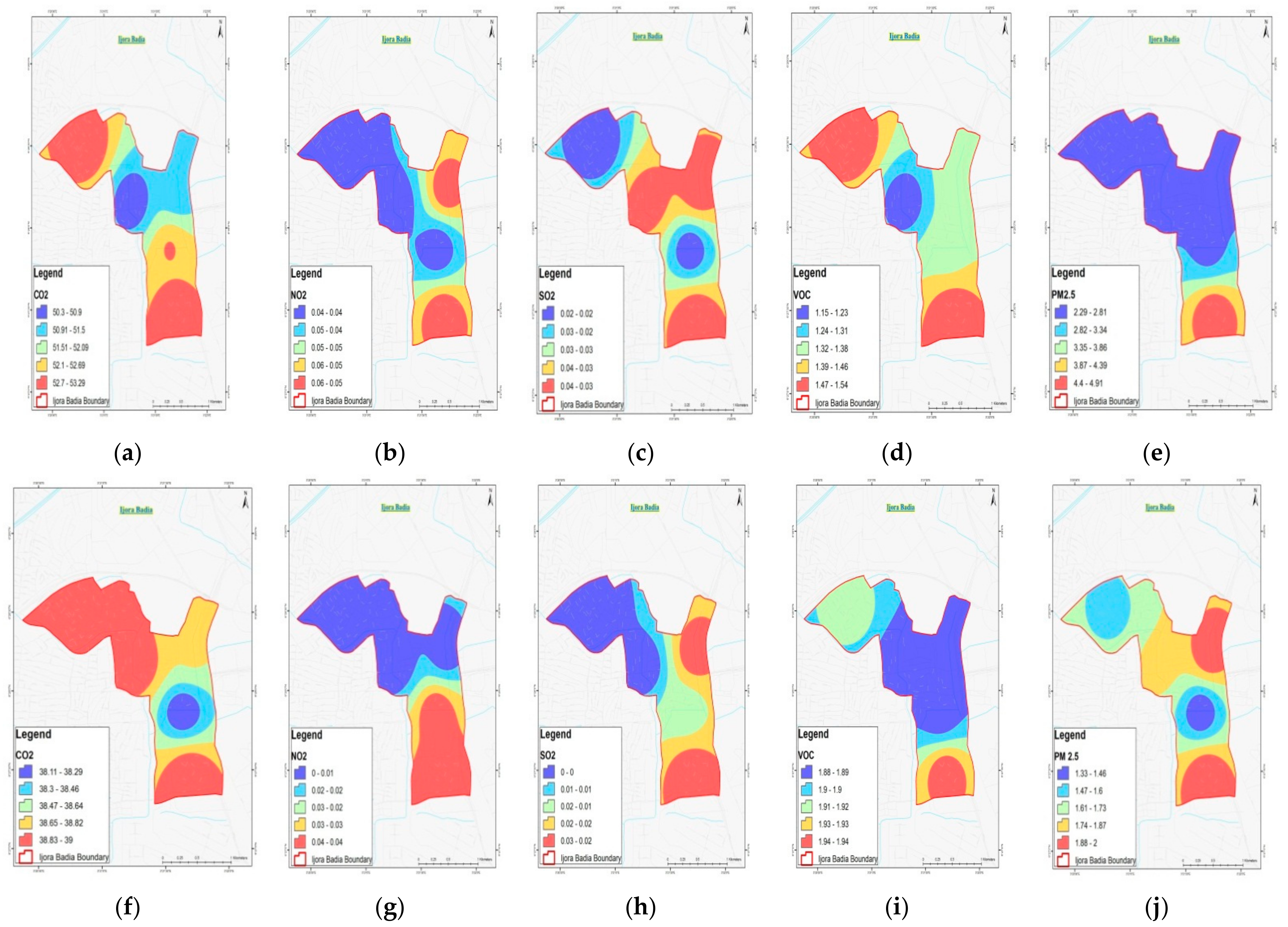
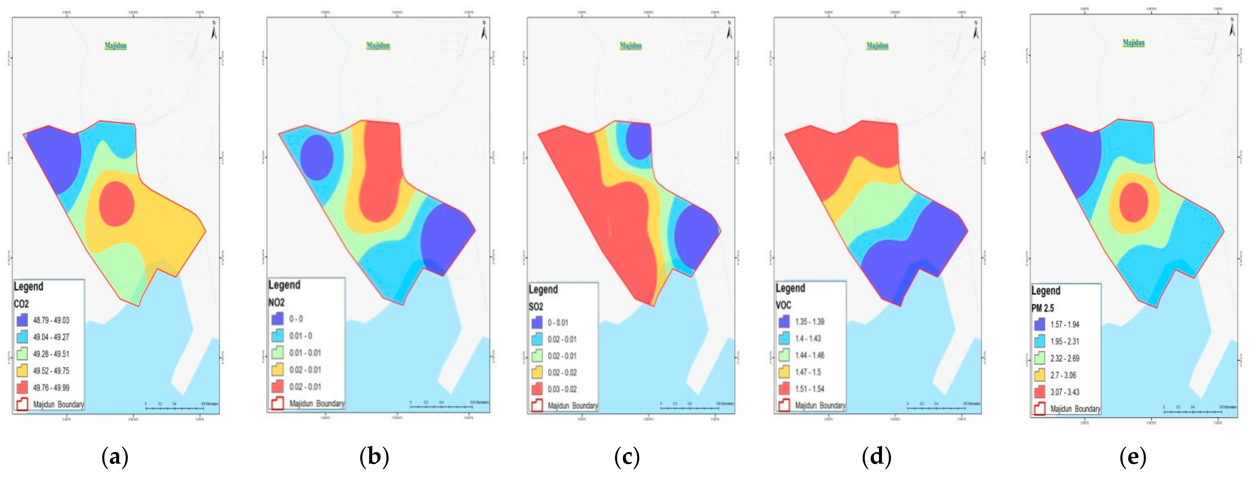
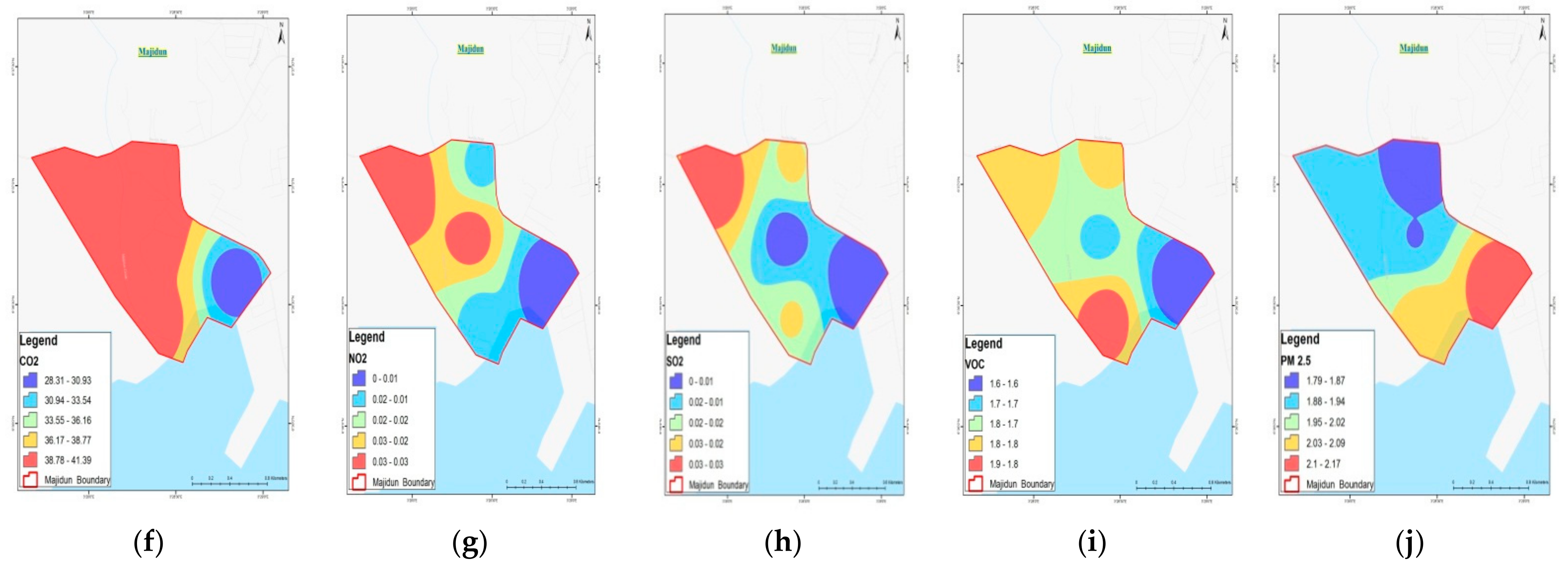
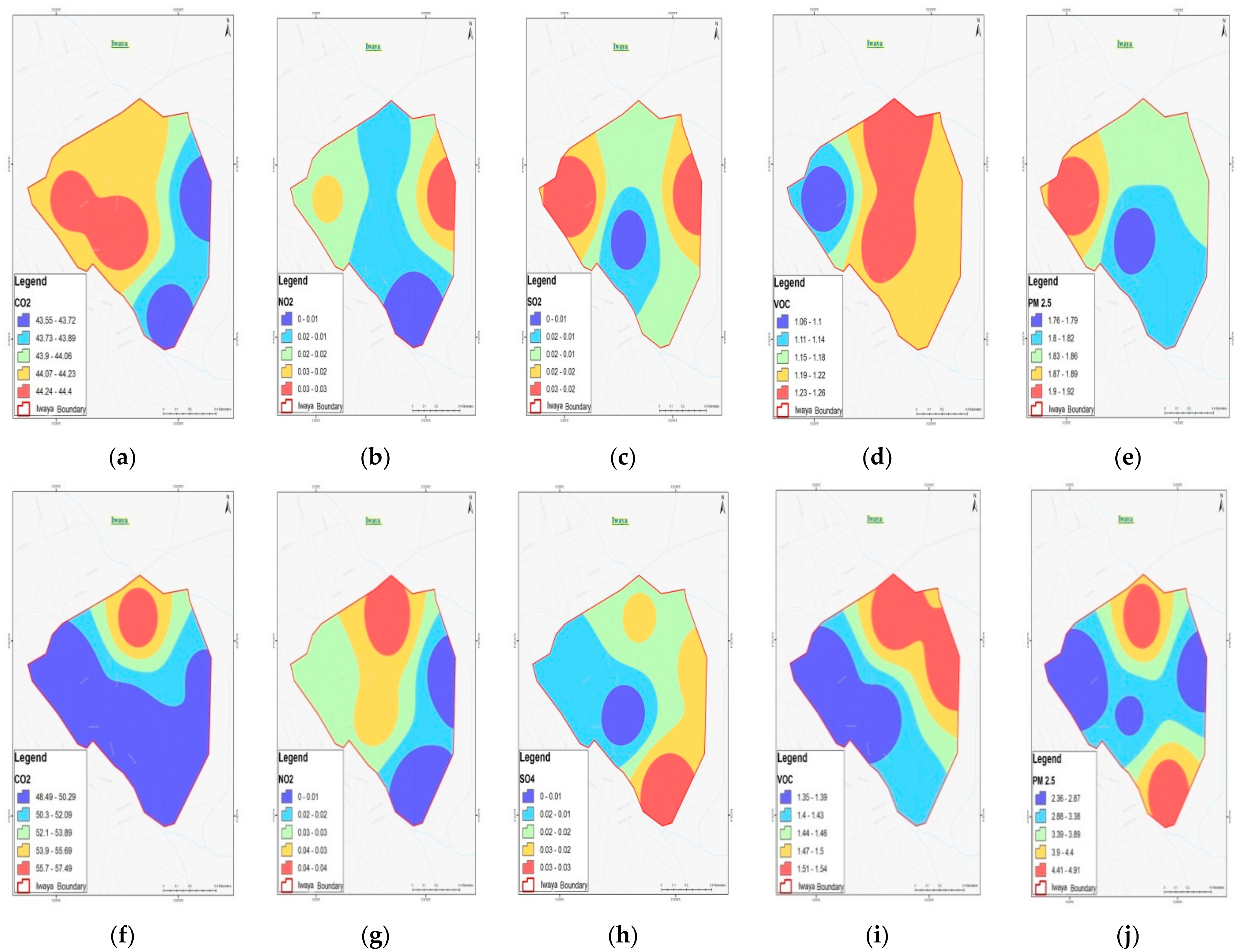
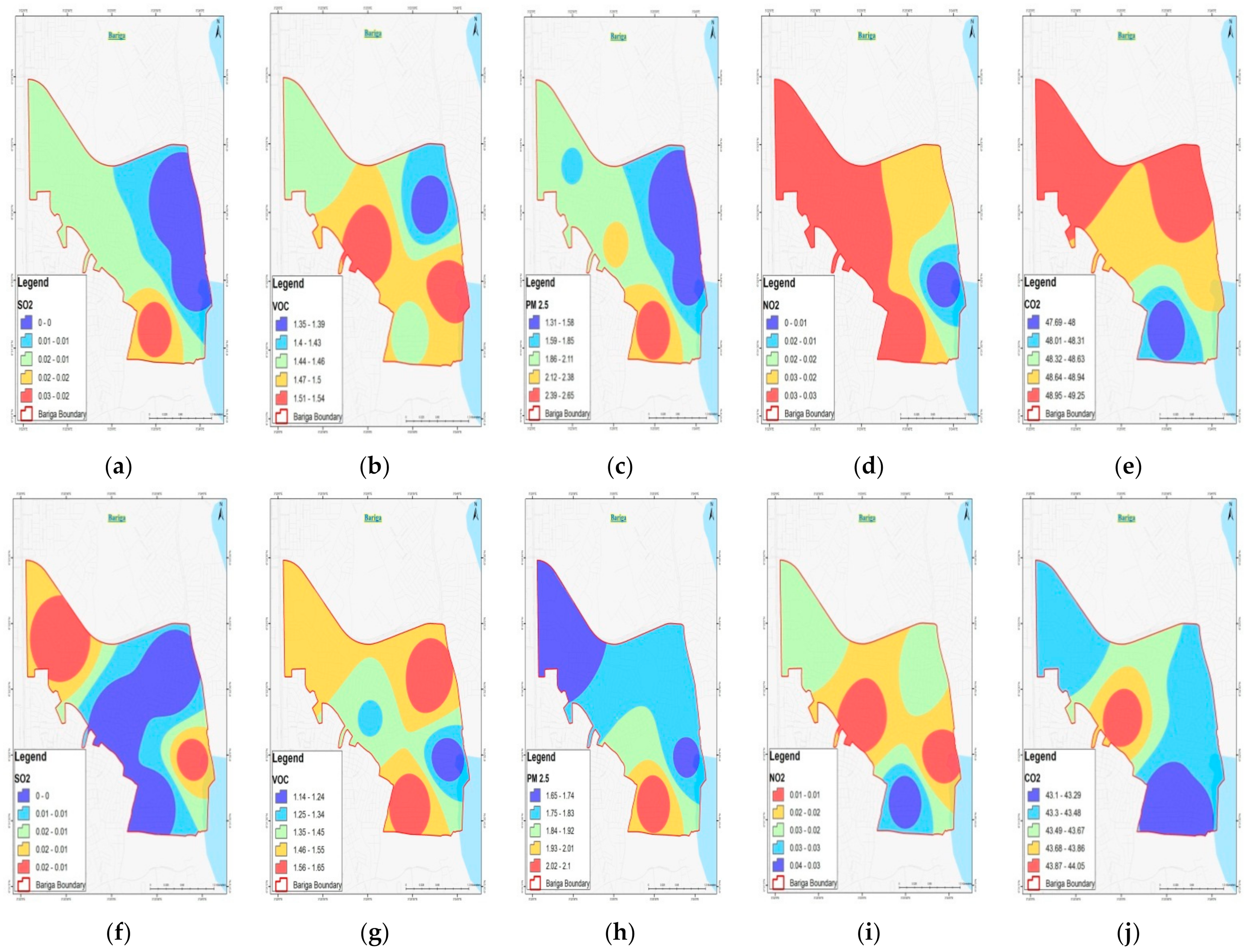
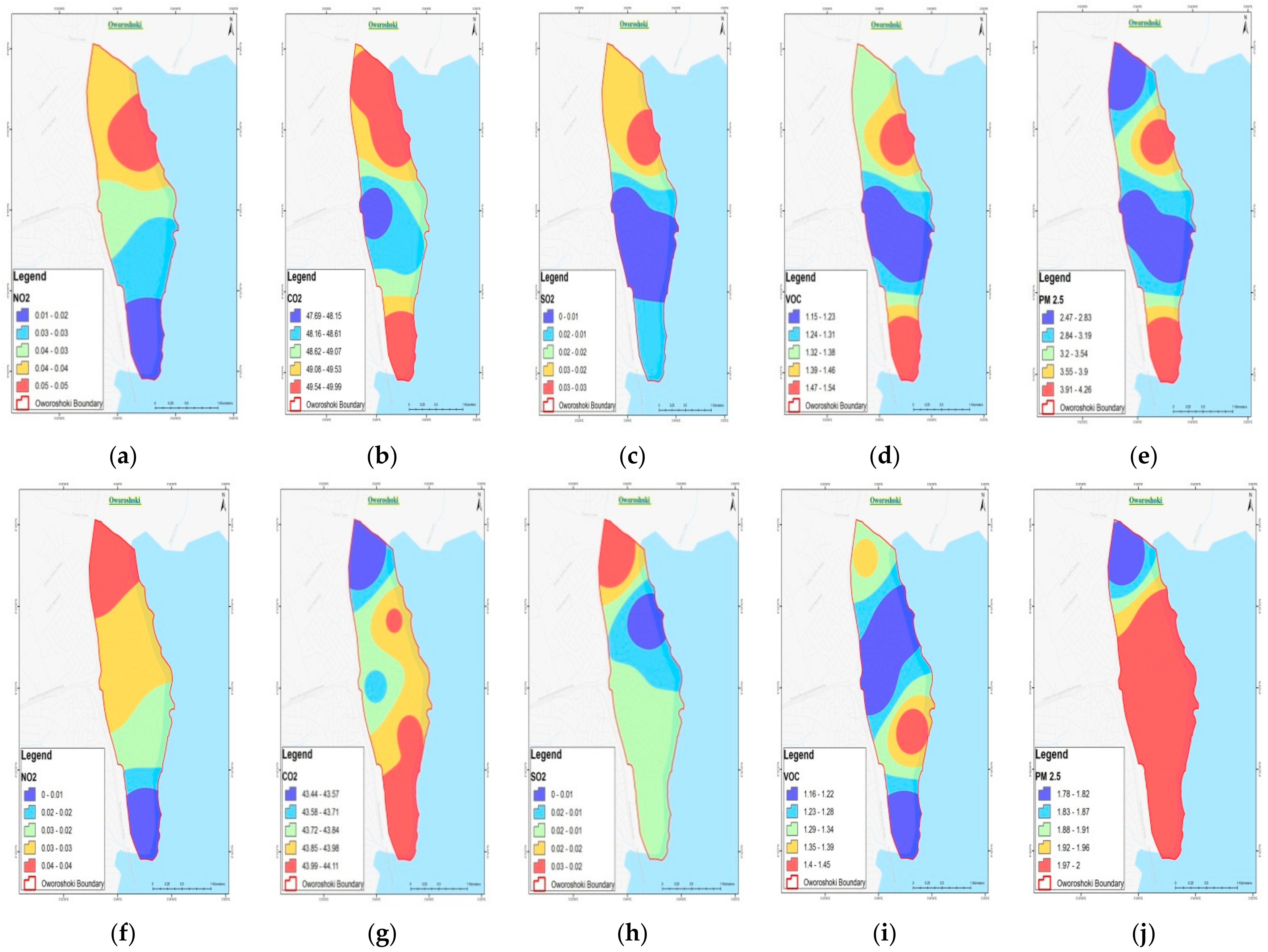
3.5. Spatial Distribution of Air Pollutants across Coastal Slum Settlements

The dispersal pattern of the air pollutant concentration level was monitored from June 2018 to May 2019 across the five selected slum settlements and is shown as five color charts on the map, representing the different concentration levels in the slum settlements (Figure 4, Figure 5, Figure 6, Figure 7 and Figure 8). There was a high to low score value recorded throughout the study area. Maps with a high Z score and a modest p-value imply a substantial hot spot location. A negative Z score and low p-value suggest a substantial cold spot [69]. In line with the spatial analysis results obtained from this study, it was evident that the dispersal pattern of pollutants from the five selected slum settlements (SA–SE) had high Z scores and modest p-values for air pollutants in the range of 49.19–57.59 (CO2), 0.03–0.05 (NO2), 0.02–0.03 (SO2), 1.41–1.54 (VOC), and 3.43–4.91 (PM2.5), signifying significant hot spot areas. The negative Z scores and low p-values of the air pollutants varied in the range of 47.69–48.79, 0.001–0.02, 0.001–0.01, 1.15–1.35, and 1.31–2.17 for CO2, NO2, SO2, VOC, and PM2.5, respectively, across the study areas; this suggested cold spot areas.
The findings from this study during the wet season showed high Z scores and a modest p-value for CO2, ranging from 39.00 to 44.40 for hot spot areas, while the values of 28.31–38.67 for a negative Z score and low p-value suggested cold spot areas across the five selected study areas (Figure 4, Figure 5, Figure 6, Figure 7 and Figure 8). NO2 showed a high Z score and a p-value that varied from 0.03 to 0.04, while the low p-score value ranged between 0.001 and 0.02. SO2 had a high Z score and p-value between 0.02 and 0.03, while 0.001–0.01 represented a negative Z score and low p-value for a cold spot area. Furthermore, VOC had a high Z score of 1.51–1.94 and p-value of 1.14–1.45. Additionally, PM2.5 had a high Z score and p-value ranging from 1.82 to 2.17, while the negative Z score and low p-value varied from 1.33 to 1.78 for cold spot areas in the Ijora-Badia, Bariga, Majidun, Iwaya, and Oworoshoki slum settlements.

4. Discussion

The findings from this study were consistent with Islam et al. [37], who reported that monthly particulate matter shows a higher concentration in dry periods (October to March) than in wet periods (April to September) in Dhaka. Usually, wet deposition due to precipitation and seasonal pollution sources are considered the main reasons for this seasonal variation [37]. The increased and decreased concentration levels of pollutants at the peak and trough during wet and dry seasons could be due to vehicular traffic, accompanied by construction/demolition activities and their related waste transfer and management, the open burning of solid waste, and secondary particle formation [70]. Trend analysis is an important tool for examining the changes in pollutant concentration over time [71] and can be used as evidence of the efficacy of policy interventions [72]. Studies have attempted to replicate this approach with more monitoring sites, such as the study by [73], which analyzed the trends in the concentration of a range of pollutants at 43 monitoring sites in the Veneto region of Italy. The authors of [72] employed a different method to examine the trends in roadside increments of various pollutants between 2005 and 2009 and 2010 and 2014, by averaging data from 65 London monitoring sites. The authors of [74] used this approach to estimate trends in particulate matter and ozone concentrations in Santiago, Chile, in 1989–1998, using data from four monitoring sites. In line with the observations of [75], environmental pollutants are emitted by large-scale human activities, thereby influencing the environment. These pollutants have different physical and chemical properties, explaining the discrepancies in their capacity for producing toxic effects. In this regard, [76] reported that the diffusion of these air pollutants is not restricted by urban boundaries; they can travel from one region to another. The findings from this study confirmed that continuous expansion, population increase, and the transformation of Lagos will contribute to increasing levels of air pollutants, thereby posing great environmental challenges to the city [13].
The authors of [77] documented that CO2 can enter into the atmosphere through municipal solid waste burning, the burning of trees and wood products, and chemical reactions. The authors of [78] also reported that the increase in anthropogenic activities is contributing immensely to outdoor pollution, and the rising level of CO2 is altering the disposition, production, and seasonal occurrence of aeroallergens. A rise in temperature of one degree caused by CO2 could increase cancer cases by 20 to 30% [79]. Exposure of the body to increased CO2 affects a person’s internal respiration, and might cause problems such as kidney damage, asphyxiation, and frostbite [80]. Additionally, adverse health effects such as suffocation, dizziness, and disorientation under certain circumstances might arise due to higher concentrations of CO2 in residential settlements [81].
The findings from this study imply that harmful emitted SO2 gases can be attributed to fossil fuel consumption or industrial activities. The authors of [82] ascertained that SO2 emissions are also a precursor to acid rain and atmospheric particulates. The authors of [83] showed that increased vehicle populations can be associated with SO2 emissions, since the combustion of fossil fuels creates SO2 emissions into the atmospheric environment. The authors of [84] stressed that anthropogenic activities are the main automobilist of air pollution emissions, adding to the pre-existing sources of natural emissions. However, [85] found that the health effects of these pollutants depend on the area, season, country, and time. Multiple cardiovascular health problems have been observed following exposure to air pollutants. The authors of [86] also reported that SO2 plays a significant role in respiratory symptoms in the healthy and in patients with underlying pulmonary disease, with symptoms such as coughing and wheezing, bronchitis, mucus production, and bronchospasm. In their work, the authors of [87] demonstrated that empirical SO2 exposure alters airway physiology, increasing airway resistance and increasing the risk of lung cancer in non-smokers. Furthermore, the authors of [88] conducted a study in China, where they found that SO2 may contribute to the risk of lung cancer mortality. The circulatory system is especially susceptible to toxins in exhaust fumes, and exposure has been linked to anemia and asphyxiation [89]. The toxicity of several air contaminants may also be related to numerous cancers in the long term [90].
The results of this study revealed that high levels of PM2.5 in these slums might be attributed to vehicular exhaust, due to the fairly dense traffic on major roads and bus stops. The authors of [91] reported that in arid regions in Asia, Africa, Latin America, and Australia, the main sources of PM2.5 in ambient air vary, but it can remain in the air for long periods. However, [92] reported that PM2.5 concentrations are higher in central urban areas because of the high-density built environment and human activities, with levels gradually decreasing toward the urban fringe. The authors of [93] also ascertained that variations in PM2.5 levels occur from site to site, based on the overall planning and layout of a city, landform [94], imminent built environment characteristics, and traffic [95], along with other human-related activities [96]. Furthermore, many epidemiological studies have confirmed the relationship between increased mortality and morbidity and higher PM2.5 concentrations [97]. A recent US study found that long-term exposure to ambient PM2.5 was associated with an elevated risk of mortality in nationwide adult cohorts [98]. Recently, approximately one million premature deaths yearly were attributed to atmospheric fine particle pollution worldwide [99]. An estimated 3.5 million COPD and 220,000 lung cancer deaths result from anthropogenic PM2.5 annually [100].
The high values recorded in this study could be attributed to traffic-related pollutants emitted from automobile engines [101], combustion processes, and industrial activities [102], which have emerged as the most significant atmospheric air contaminants connected to health problems such as chronic lung disease as a result of long-term exposure. However, systems other than respiratory organs can be involved; symptoms such as throat, nose, and eye irritation have been registered [103]. Recent epidemiological studies discovered that exposure to nitrogen dioxide early in life may lead to allergic diseases [104] and have a long-term impact on lung functional respiratory health throughout the lifetime [105]. The most vulnerable sub-group to NO2 is children, because they inhale more air than adults relative to their body size and have greater metabolic activity [106]. Poor air quality, either outdoors or indoors, can adversely affect the human respiratory and cardiovascular systems [107].
The results from this study showed that VOCs are released from both natural and man-made sources due to their elevated volatility under normal atmospheric conditions [108]. The International Agency for Research on Cancer (IARC) classifies VOCs such as benzene, 1,3-butadiene, and vinyl chloride as Group 1 carcinogens for humans [109]. There is evidence to support the idea that there is a link between environmental pollution and acute myeloid leukemia in children, particularly due to benzene exposure [110]. As a result, prolonged exposure to VOCs may be harmful to health [111]. VOCs are associated with neurological toxicity, kidney malfunction, acute and chronic respiratory disorders, irritation of the nose, throat, and eyes, headaches, nausea, dizziness, and allergic skin reactions, as well as damage to internal organs such as the liver and kidneys [112]. Simultaneous exposure to other VOCs may worsen other disease symptoms [113], through a synergistic effect on oxidative stress induction from exposure to toluene, chloroform, and dichloromethane. This type of exposure may also affect the fetal endocrine system [114], by altering the developmental process of the fetus. The authors of [115] commissioned a pollution and health study and reported that an estimated five to six million deaths occurred worldwide in 2015 due to modern environmental pollution.
The observed correlations among the air pollutants, especially VOC, CO2, and SO2 in the wet season and NO2 and SO2 during the dry season, may be due to their relatively common source [116]. The findings from this study confirmed that under high humidity conditions, semi-volatile species and aerosols can more easily be absorbed, leading to an increase in particulate matter concentrations [117]. In addition, high relative humidity favors the formation of temperature inversion, which stabilizes the atmospheric stratification and hinders the vertical diffusion of pollutants [118]. The values of NO2 were negatively correlated with temperature due to the transformation of NO2 to O3 and the high temperature under vertical dispersion conditions in [119]. Conversely, air pollutant variables in this study showed strong positive and negative correlations with meteorological parameters such as relative humidity, ambient temperature, and atmospheric pressure in both the wet and dry seasons (Table 2 and Table 3). The results of this study showed that PM2.5 had a significant positive correlation with temperature during the wet season; on the contrary, Islam et al. [37] reported an insignificant positive correlation with PM2.5 (r = 0.06, p = 0.734) during the wet season in Dhaka. An inverse relationship was found between PM2.5 and temperature in the literature [120], which indicates the cooling effect of particulate matter due to its negative radioactive forces [37]. Air pollutants can become airborne from the ground surface when they are emitted from an elevated stack, and they can be formed in the atmosphere as secondary particulate matter [37]. The findings from this study also showed that relative humidity was negatively correlated with temperature during the wet season, which is consistent with the results obtained from Dhaka city, where relative humidity was negatively correlated with PM2.5 in all periods (r = −0.48, −0.58, and −0.61, respectively, for the dry-1, wet, and dry-2 periods, p < 0.05 in all cases) [37]. The negative relationship found between PM2.5 and relative humidity during the wet and dry seasons showed the growth and posterior wet precipitation of particles, as observed in Dhaka [30], compared to the findings from this study. Other studies [37,38,39] have distinguished the effect of relative humidity on PM2.5. However, relative humidity can influence particles, where the gathered mass settles on the ground; the particulate matter average mass concentration has been shown to have a decreasing trend with an increase in ambient relative humidity [121]. High relative humidity has been found to favor the partition of semi-volatile species into the aerosol phase [120], leading to high particulate matter concentrations. A moister atmosphere usually accompanies a lower boundary layer [122], which additionally enhances the concentrations of primary source pollutants. NO2, SO2, and CO2 play a major role in producing O3 in the environment [123]. Although all combustion in air can produce this chemical compound, it relies on the composition of nitrogen in the combustion emissions [124]. Researchers [125] have found similar results to this study. Several studies have applied a correlation statistical tool to air pollution in Chicago [126], performed isotopic analyses in topsoil [127], and identified sources and correlations between PAHs and heavy metals in Switzerland and Spain [128], and in the urban road dust of Xi’an (China) [129]. The interactions between meteorological and air pollutant parameters are quite complex, vary seasonally, and are often influenced by the local physiography variations, such as the location of mountains and valleys, and the presence of substantial water bodies (rivers and lakes) [130]. The findings from this study revealed that air pollution mainly affects those living in large urban areas, where most people still generate their electricity through fossil fuel (diesel and petrol) for both commercial and domestic use, and road vehicular emissions contribute the most to the degradation of air quality [131].
The regression model of this study showed that temperature, atmospheric pressure, and relative humidity had a higher predictive power for the air pollutant parameters compared to the results obtained in Dhaka, with a low predictive power (adjusted r2 = 0.35). The study conducted in Dhaka city suggested that meteorological variables have a minor impact on the coarser particulate matter fraction compared to the finer fraction [30]. Atmospheric pressure, relative humidity, and temperature are the most significant predictors of the model used in this study, and their associations with the air pollutant parameters correspond to other studies conducted in Dhaka [37]. A study conducted in Xi’an showed that the contribution of SO2 to PM2.5 outweighed that of NO2, which implies that the main polluting gas was SO2 [17]. Research has also shown that 31% of NO2 contributes 10% of the total PM2.5 in air pollutants, especially from traffic, while 73% is emitted from power plants, accounting for 12% of the total PM2.5 in the year 2003 in the Huabei region, China [132]. The SO2 and NO2 contribution to PM2.5 in the year 2010 in Xi’an showed a different pattern compared to that recorded in 2003 in the Huabei region, while other studies showed that SO2 emissions started decreasing in China after 2006 [133]. In this context, [134] documented that Shanghai had a significant linear increase in NO2 concentrations, with approximately a 20% increase rate annually during the period of 1996–2005, while [135] noted that satellite observations and model simulation could also be used to detect and predict strong increases in NO2 in Eastern China. Accordingly, [133] found that SO2 from local coal-burning power plants is the primary contributor to air pollutants, produced from west–east electricity transmission and raw material-based projects in Xi’an. However, the findings from this study confirmed that meteorological factors can impact pollutant concentrations, and the exposure level of particle mixtures of pollutants can change throughout the year [136]. The heat from solar radiation is absorbed by the air, minimizing the atmospheric temperature near the Earth’s surface. The air layer nearer to the Earth’s surface becomes colder than the upper layers, thereby reducing the air currents moving upwards, leading to an increase in pollutant concentrations [137]. Generally speaking, this could explain the positive and moderately correlated air pollutant and meteorological parameters obtained in the wet and dry seasons. Several studies across the globe have assessed the link between meteorological processes and air pollution variables. The authors of [138] studied the effect of meteorological variables, including rainfall, on particulate concentration, and found that suspended particulate matter and PM10 had a negative correlation with rainfall at Ahmedabad in India. The authors of [139] also studied the effects of seasonal variation on particulates in Delhi, and found that the suspended particulate matter concentration was inversely related to relative humidity in all seasons. The authors of [121] studied the relationship between meteorological processes and air pollution in Kathmandu in Nepal, and found that an increase in humidity has a negative correlation with the concentration of PM2.5. The authors of [17] reported the benefits of air quality enhancement zone establishments in Taiwan, including CO2 capture, carbon storage, and global warming mitigation. However, the harmful effects of air pollution and its causes have been widely studied worldwide [140]. Air pollution is influenced by multiple environmental and meteorological factors, as well as traffic patterns, size, land use, and the orientation of buildings [141]. The findings from this study showed that the growth of these slum settlements is associated with anthropogenic activities that impact the urban environment [142].
The dispersion of pollutants can be affected by multiple variables [143]. Pollutant dispersion patterns can also provide information for an environmental health impact appraisal [144]. The obtained information from the maps shows that pollutants at different locations express different emission patterns across the slum settlements.
Additionally, the appearance of spatial clusters of pollutants in these areas suggests locations for the aggregation of contaminants, rather than representing the origin of emissions, which is influenced by geographical and climatological conditions. Several studies have applied the kriging and Getis–Ord approach to identify different levels of spatial clusters. The authors of [145] estimated vehicle emissions for major traffic routes, and evaluated their spatial pattern by applying the global Moran’s I and Getis tests. Spatial resolutions varied for one monitor [146] in high-density sampling campaigns [147]. However, Wang et al. [148] used the ordinary kriging method to estimate the spatial characteristics of PM across Beijing from 2008 to 2009. Liang et al. [149] suggested the use of hotspot-based spatial monitoring systems to further understand the mechanisms underlying the observed relationship between health and environmental policy implications. Spatial resolution should be adopted when carrying out air pollution monitoring appraisement.

5. Conclusions

This study revealed the effects of air pollutants and their associated health hazards on slum residents between June 2018 and May 2019 in the coastal slum settlements of the Lagos metropolis. The seasonal variation in air pollutants showed that SO2, NO2, CO2, and PM2.5 had higher trend patterns of pollution concentrations during the dry season than the wet season. A strong correlation was found between PM2.5 and temperature at the 1% level (0.957 **), and between VOC and SO2 (0.907 *) at the 5% level, during the wet season. Furthermore, during the dry season, a positive correlation existed between NO2 and SO2 at the 1% level (0.9477 **), as well as between PM2.5 and relative humidity (0.832 *) at the 5% level. The influence of meteorological parameters on air pollutants showed that the major predictive factors for the dispersion pattern of VOC, CO2, and SO2 were relative humidity, temperature, and atmospheric pressure, at a rate of 92.6%, 99.7%, and 100% and 72.0%, 60.7%, and 98.4% during the wet and dry seasons, respectively. Spatial analysis revealed that the dispersal pattern of air pollutants showed a high Z score and a modest p-value in Bariga, Majidun, and Oworoshoki. Most of these slum settlements showed clustering of pollutants in some parts of the communities, indicating likely locations for the accumulation of pollutants in hot spot zones. In addition, the Iwaya and Ijora-Badia slums recorded negative Z scores and low p-values in most parts of the settlement. The different patterns of clustering across the study area showed areas of lesser accumulation of pollutants, known as cold spot areas. Although this study captured the applicability of the kriging and Getis–Ord general G statistics interpolation method to map and quantitatively link the patterns and processes of air pollutants in the slum settlements of Lagos, there is scope for further improvement. The remotely sensed data utilized in this study covered two periods (wet and dry seasons) due to limited data availability, and covered a few selected slum settlements in Lagos, preventing the interval level of intensity analysis. A broader coverage, including all identified slum settlements and more years of remotely sensed data, could give further insight into air pollutant concentrations and their relationship with meteorological variables in the slum settlements of Lagos, Nigeria. Integrating spatial analysis in GIS and statistical modeling could help researchers to expand the understanding of the distribution of air pollutants in a location or area, in order to understand the factors that influence the trends and significance of ambient air pollution. The spatial map can also provide an overview of the potential risks experienced by slum dwellers exposed to high levels of air pollutants in certain areas.
The findings imply that the spatial and meteorology-based air quality model developed for monitoring the slum settlements cannot be applied to other sites. This study clearly showed that the location of pollution sources with respect to densely populated urban centers may play an important role in determining their adverse impacts. These results indicate that atmospheric pressure, relative humidity, and temperature can be contributing factors in governing air pollutant concentrations in the slum settlement. Some of these meteorological events are not completely dissociative; for instance, increased humidity would naturally be positively correlated with rainfall events, and hence drawing a conclusion based on a particular meteorological parameter to predict the air pollutant concentration would be unwise. A follow-up investigation of the impact of meteorological variables on air pollutants in slum settlements is warranted once proper meteorological observations are available. The kriging and Getis–Ord general G statistics interpolation method presented here that was used to predict the movement of air pollutant parameters from slum A to other slum locations within the Lagos metropolis has other implications as well. The concentration of air pollutants can be forecast from the model used for this study if the meteorological variables and air pollutant concentration data of a city are known. A retrospective analysis of air pollutant trends in slum settlements where air pollutant concentration data were not reported or were missing for a certain period of interest can also be achieved. Air pollutant and meteorology models can be developed through the predictive power of the model, as indicated by their respective adjusted r2 values; however, the predictions will have uncertainty. The predicted variables should be used cautiously, acknowledging their limitations. Additionally, the model is centered on the meteorological and air quality data of slum settlements in Lagos only; thus, care is necessary when using it for other geographical localities, where emission scenarios and meteorological conditions may be different.
In Lagos State, ambient air monitoring remains unregulated and uncoordinated, despite the efforts of local researchers and relevant government agencies, such as the National Environmental Standards and Regulatory Agency and Nigerian Metrological Agency. Therefore, it is recommended that a national air quality monitoring network be established in important urban areas, including the slum settlements in Lagos. Fixing emission caps and taxes for industries based on identifiable economic costs and advantages to public health and quality of life is required. This would support new, rational, and scientific regulations, policies, and advancements to combat air pollution. Finally, the findings from this study provide valuable information on environmental pollution sources that could aid environmental legislators in the decision-making process.

Author Contributions

O.P.O.: Conceptualization, Methodology, Software, Investigation, and Writing—Original Draft Preparation. K.T.: Supervision, Project Administration. J.N.S.: Reviewing, Editing, and Formal Analysis. O.O.T.-A.: GIS Software Analysis. A.T.O.: Data Curation and Investigation. M.A.A.: Software, Validation, and Writing—Reviewing and Editing. K.P.: Final Draft Preparation, Supervision, and Funding Acquisition. All authors have read and agreed to the published version of the manuscript.

Funding

This research was supported by Prince of Songkla University and the Ministry of Higher Education, Science, Research, and Innovation under the Reinventing University Project (Grant Number REV64023).

Institutional Review Board Statement

Not applicable.

Informed Consent Statement

Not applicable.

Data Availability Statement

National Emission Standards for Hazardous Air Pollutants for Source Categories. Portland Cement Manufacturing Industry. Federal Register https://www.gpo.gov/fdsys/pkg (accessed on 14 June 2018); Lagos Water Regulatory Commission (LSWRC). (2016). Introduction. Retrieved from http://lswrc.lagosstate.gov.ng/2016/06/10/introduction-2/ (accessed on 25 September 2021); 66. NAAQS 2O12. Criteria Air Pollutants Ambient Standards. https://epa.gov (accessed on 30 June 2021).

Acknowledgments

The contributions and resources of the authors and all the co-authors of this publication are gratefully acknowledged. This research was supported by Prince of Songkla University and the Ministry of Higher Education, Science, Research, and Innovation under the Reinventing University Project (Grant Number REV64023).

Conflicts of Interest

The authors declare that they have no known competing financial interests or personal relationships that could have appeared to influence the work reported in this paper.

References

  1. Borck, R.; Schrauth, P. Population density and urban air quality. Reg. Sci. Urban Econ. 2021, 86, 103596. [Google Scholar] [CrossRef]
  2. Landrigan, P.J. Air pollution and health. Lancet Public Health 2017, 2, e4–e5. [Google Scholar] [CrossRef] [Green Version]
  3. Phoungthong, K.; Tekasakul, S.; Tekasakul, P.; Prateepchaikul, G.; Jindapetch, N.; Furuuchi, M.; Hata, M. Emissions of particulate matter and associated polycyclic aromatic hydrocarbons from agricultural diesel engine fueled with degummed, deacidified mixed crude palm oil blends. J. Environ. Sci. 2013, 25, 751–757. [Google Scholar] [CrossRef]
  4. Phoungthong, K.; Tekasakul, S.; Tekasakul, P.; Furuuchi, M. Comparison of particulate matter and polycyclic aromatic hydrocarbons in emissions from IDI-turbo diesel engine fueled by palm oil–diesel blends during long-term usage. Atmos. Pollut. Res. 2017, 8, 344–350. [Google Scholar] [CrossRef]
  5. Godehart, S.; Vaughan, A. Research Reviewing the Bng in Relation to Upgrading Informal Settlements. In Research Paper for Theme 1: Conceptual Framework; The National Department of Housing, Singapore Institute of Management (SIM): Singapore, 2008; p. 20. [Google Scholar]
  6. FGN-MDG Report. The Millennium Development Goals Report: We Can End Poverty; United Nations: New York, NY, USA, 2010; Available online: http://www.mdgreport.org (accessed on 15 January 2010).
  7. Agbola, T.; Agunbiade, E.M. Urbanization, slum development and security of tenure: The challenges of meeting millennium development goal 7 in metropolitan Lagos, Nigeria. In Urban Population-Environment Dynamics in the Developing World: Case Studies and Lessons Learned; Committee for International Cooperation in National Research in Demography (CICRED): Paris, France, 2009; pp. 77–106. Available online: http://www.populationenvironmentresearch.org/workshops.jsp#W2007 (accessed on 21 October 2019).
  8. George, C.K. The Challenges of Urbanization in Nigeria Urban Centres: A Review of the Physical Planning Development of Lagos Megalopolis. In Proceedings of Architects Colloquium; Architects Registration Council of Nigeria: Abuja, Nigeria, 2008; pp. 74–95. [Google Scholar]
  9. Falade, J.B. The Role of Physical Planning in a Megacity. In Paper Presented on the Theme: Towards a Harmonius Megacity Organized by the Lagos State Government during the 2008 World Habitat Day at the Lagos State Secretariat, Ikeja; Federal Ministry of Power, Works and Housing: Abuja, Nigeria, 2008; pp. 1–12. [Google Scholar]
  10. UN-Habitat; (United Nations Human Settlements Programme). State of the World’s Cities 2010/2011-Cities for All: Bridging the Urban Divide; Earthscan Publishers: Nairobi, Kenya, 2008; Available online: www.unhabitat.org (accessed on 10 March 2018).
  11. Ojiodu, C.C.; Okuo, J.M.; Olumayede, E.G. Spatial and temporal variability of volatile organic compounds (VOCs) pollution in Appa industrial areas of Lagos state, Southwestern-Nigeria. J. Acad. Environ. Sci. 2013, 1, 53–61. [Google Scholar]
  12. Do, D.H.; Van Langenhove, H.; Walgraeve, C.; Hayleeyesus, S.F.; De Wispelaere, P.; Dewulf, J.; Demeestere, K. Volatile organic compounds in an urban environment: A comparison among Belgium, Vietnam and Ethiopia. Int. J. Environ. Anal. Chem. 2013, 93, 298–314. [Google Scholar] [CrossRef]
  13. Olowoporoku, A.; Longhurst, J.; Barnes, J. Framing Air Pollution as a Major Health Risk in Lagos, Nigeria. In Air Pollution XX; Brebbia, C., Longhurst, J., Eds.; WIT Press: Southampton, UK; Boston, MA, USA, 2012; pp. 479–486. ISBN 9781845645823. [Google Scholar]
  14. Kumar, P.; Yadav, S. Seasonal variations in water soluble inorganic ions, OC and EC in PM10 and PM>10 aerosols over Delhi: Influence of sources and meteorological factors. Aerosol Air Qual. Res. 2016, 16, 1165–1178. [Google Scholar] [CrossRef] [Green Version]
  15. Suvarapu, L.N.; Seo, Y.K.; Baekm, S.O. Volatile organic compounds and polycyclic aromatic hydrocarbons in ambient air of Indian cities—A review. Res. J. Chem. Environ. 2013, 17, 67–75. [Google Scholar]
  16. Luken, R.A.; Van Berkel, R.; Leuenberger, H.; Schwager, P. A 20-year retrospective of the national cleaner production centres programme. J. Clean. Prod. 2016, 112, 1165–1174. [Google Scholar] [CrossRef]
  17. Wang, P.; Cao, J.; Tie, X.; Wang, G.; Li, G.; Hu, T.; Wu, Y.; Xu, Y.; Xu, G.; Zhao, Y.; et al. Impact of Meteorological Parameters and Gaseous Pollutants on PM2.5 and PM10 Mass Concentrations during 2010 in Xi’an, China. Aerosol Air Qual. Res. 2015, 15, 1844–1854. [Google Scholar] [CrossRef] [Green Version]
  18. Zhou, H.; Yu, Y.; Gu, X.; Wu, Y.; Wang, M.; Yue, H.; Gao, J.; Lei, R.; Ge, X. Characteristics of Air Pollution and Their Relationship with Meteorological Parameters: Northern Versus Southern Cities of China. Atmosphere 2020, 11, 253. [Google Scholar] [CrossRef] [Green Version]
  19. Wang, X.-C.; Klemeš, J.J.; Dong, X.; Fan, W.; Xu, Z.; Wang, Y.; Varbanov, P.; Reviews, S.E. Air pollution terrain nexus: A review considering energy generation and consumption. Renew. Sust. Energ. Rev. 2019, 105, 71–85. [Google Scholar] [CrossRef]
  20. Ma, Y.; He, W.; Zhao, H.; Zhao, J.; Wu, X.; Wu, W.; Li, X.; Yin, C. Influence of Low Impact Development practices on urban diuse pollutant transport process at catchment scale. J. Clean. Prod. 2019, 213, 357–364. [Google Scholar] [CrossRef]
  21. Zhong, Q.; Ma, J.; Shen, G.; Shen, H.; Zhu, X.; Yun, X.; Meng, W.; Cheng, H.; Liu, J.; Li, B.; et al. Distinguishing Emission-Associated Ambient Air PM2.5 Concentrations and Meteorological Factor-Induced Fluctuations. Environ. Sci. Technol. 2018, 52, 10416–10425. [Google Scholar] [CrossRef] [Green Version]
  22. Liu, X.; Nie, D.; Zhang, K.; Wang, Z.; Li, X.; Shi, Z.; Wang, Y.; Huang, L.; Chen, M.; Ge, X.; et al. Evaluation of particulate matter deposition in the human respiratory tract during winter in Nanjing using size and chemically resolved ambient measurements. Air Qual. Atmos. Health 2019, 12, 529–538. [Google Scholar] [CrossRef]
  23. Meng, C.; Cheng, T.; Gu, X.; Shi, S.; Wang, W.; Wu, Y.; Bao, F. Contribution of meteorological factors to particulate pollution during winters in Beijing. Sci. Total Environ. 2019, 656, 977–985. [Google Scholar] [CrossRef]
  24. He, J.; Gong, S.; Yu, Y.; Yu, L.; Wu, L.; Mao, H.; Song, C.; Zhao, S.; Liu, H.; Li, X.; et al. Air pollution characteristics and their relation to meteorological conditions during 2014–2015 in major Chinese cities. Environ. Pollut. 2017, 223, 484–496. [Google Scholar] [CrossRef] [PubMed]
  25. Chan, C.K.; Yao, X. Air Pollution in Mega Cities in China. Atmos. Environ. 2008, 42, 1–42. [Google Scholar] [CrossRef]
  26. Zhang, Q.; Tie, X.; Lin, W.L.; Cao, J.J.; Quan, J.N.; Ran, L.; Xu, W.Y. Measured Variability of SO2 in an Intensive Fog Event in the NCP Region, China; Evidence of High Solubility of SO2. Particuology 2013, 11, 41–47. [Google Scholar] [CrossRef]
  27. Cobourn, W.G. An enhanced PM2.5 air quality forecast model based on nonlinear regression and back-trajectory concentrations. Atmos. Environ. 2010, 44, 3015–3023. [Google Scholar] [CrossRef]
  28. Liu, Y.; He, K.; Li, S.; Wang, Z.; Christiani, D.C.; Koutrakis, P. A statistical model to evaluate the effectiveness of PM2.5 emissions control during the Beijing 2008 Olympic Games. Environ. Int. 2012, 44, 100–105. [Google Scholar] [CrossRef]
  29. Liang, X.; Zou, T.; Guo, B.; Li, S.; Zhang, H.; Zhang, S.; Huang, H.; Chen, S.X. Assessing Beijing’s PM2.5 pollutions: Severity, weather impact, APEC and winter heating. Proc. R. Soc. Lond. Ser. 2015, 471, 20150257. [Google Scholar] [CrossRef] [Green Version]
  30. Afrin, S.; Islam, M.; Ahmed, T. A Meteorology Based Particulate Matter Prediction Model for Megacity Dhaka. Aerosol Air Qual. Res. 2020, 21, 200371. [Google Scholar] [CrossRef]
  31. Badmos, O.S.; Rienow, A.; Callo-Concha, D.; Greve, K.; Jürgens, C. Urban Development in West Africa—Monitoring and Intensity Analysis of Slum Growth in Lagos: Linking Pattern and Process. Remote Sens. 2018, 10, 1044. [Google Scholar] [CrossRef] [Green Version]
  32. Adama, O. Slum upgrading in the era of World-Class city construction: The case of Lagos, Nigeria. Int. J. Urban Sustain. Dev. 2020, 12, 219–235. [Google Scholar] [CrossRef] [Green Version]
  33. Obaitor, O.S.; Lawanson, T.O.; Stellmes, M.; Lakes, T. Social Capital: Higher Resilience in Slums in the Lagos Metropolis. Sustainability 2021, 13, 3879. [Google Scholar] [CrossRef]
  34. Wang, J.; Maduako, I. Spatio-temporal urban growth dynamics of Lagos Metropolitan Region of Nigeria based on Hybrid methods for LULC modeling and prediction. Eur. J. Remote Sens. 2018, 51, 251–265. [Google Scholar] [CrossRef] [Green Version]
  35. Lagos-State/UNCHS. Identification of Urban Renewal Areas in Metropolitan Lagos; Lagos—State/UNCHS: Lagos, Nigeria, 1984. [Google Scholar]
  36. Afrin, S.; Islam, M.M.; Ahmed, T.; Ali, M.A. The influence of meteorology on particulate matter concentration in the air of Dhaka City. In Proceedings of the 2nd International Conference on Advances in Civil Engineering (ICACE-2014), Dubai, United Arab Emirates, 1–2 October 2014. [Google Scholar]
  37. Islam, M.M.; Afrin, S.; Ahmed, T.; Ali, M.A. Meteorological and seasonal influences in ambient air quality parameters of Dhaka city. J. Civ. Eng. 2015, 43, 67–77. [Google Scholar]
  38. Islam, N.; Saroar, M.G.; Ahmed, T. Meteorological influences on atmospheric particles in Darus Salam Area of Dhaka City. In Proceedings of the 4th International Conference on Civil Engineering for Sustainable Development (ICCESD), Khulna, Bangladesh, 9–11 February 2018; pp. 1–12. Available online: http://www.iccesd.com/proc_2018/Papers/r_p4167.pdf (accessed on 15 July 2020).
  39. Kayes, I.; Shahriar, S.A.; Hasan, K.; Akhter, M.; Kabir, M.M.; Salam, M.A. The relationships between meteorological parameters and air pollutants in an urban environment. Glob. J. Environ. Sci. Manag. 2019, 5, 265–278. [Google Scholar] [CrossRef]
  40. Biswas, S.K.; Tarafdar, S.A.; Islam, A.; Khaliquzzaman, M. Investigation of Sources of Atmospheric Particulate Matter (APM) at an Urban Area in Bangladesh; Chemistry Division, Atomic Energy Centre: Dhaka, Bengal, 2001. [Google Scholar]
  41. Guttikunda, S. Impact Analysis of Brick Kilns on the Air Quality in Dhaka, Bangladesh. SIM-Air Work. Pap. Ser. 2009, 21, 234. Available online: www.urbanemissions.info/simair (accessed on 3 August 2019).
  42. Begum, B.A.; Biswas, S.K.; Hopke, P.K.; Cohen, D.D. Multi-element analysis and characterization of atmospheric particulate pollution in Dhaka. Aerosol Air Qual. Res. 2006, 6, 334–359. [Google Scholar] [CrossRef]
  43. Boman, J.; Gatari, M.J.; Wagner, A.; Hossaini, M.I. Elemental characterization of aerosols in urban and rural locations in Bangladesh. X-Ray Spectrom. 2005, 34, 460–467. [Google Scholar] [CrossRef]
  44. World Population Review. Lagos Population. Available online: https://worldpopulationreview.com (accessed on 20 June 2021).
  45. Lagos Water Regulatory Commission (LSWRC). Introduction. 2016. Available online: http://lswrc.lagosstate.gov.ng/2016/06/10/introduction-2 (accessed on 16 March 2020).
  46. Oyegoke, S.O.; Sojobi, A.O. Developing appropriate technique to alleviate the Ogun River network annual flooding problems. Int. J. Sci. Eng. Res. 2012, 3, 1–7. [Google Scholar]
  47. George, C.K. Challenges of Lagos as a Mega-City. 2010. Available online: http://www.allafrica.com/stories/201002221420.html (accessed on 12 July 2010).
  48. UN. World Urbanization Prospects, Population Division. New York. 2018. Available online: https://population.un.org (accessed on 19 June 2021).
  49. United Nations Development Programme. What will it take to achieve the Millennium Development Goals-An International Assessment, Goran Holmquist, External Financing of Social Protection: Opportunities and Risks. Dev. Policy Rev. 1984, 30, 5–27. [Google Scholar]
  50. Morka, F.C. A Place to Live: A Case Study of the Ijora-Badia Community in Lagos, Nigeria. Enhancing Urban Safety and Security: Global Report on Human Settlements. 2007. Available online: https://staging.unhabitat.org/downloads/docs/GRHS.2007.CaseStudy.Tenure.Nigeria.pdf (accessed on 15 July 2017).
  51. Olulade, P. Assessing the Lagos Megacity Selected Slum Settlements Housing and Environmental Conditions. J. Multidiscip. Eng. Sci. Technol. 2016, 3, 5408–5416. [Google Scholar]
  52. Action Health Incorporated. A Promise to Keep: Supporting Out-of-School Adolescent Girls to Reach Their Potential; Action Health Incorporated and Lagos State Ministry of Education: Lagos, Nigeria, 2011. [Google Scholar]
  53. Kunnuji, M.O. Experience of domestic violence and acceptance of intimate partner violence among out-of-school adolescent girls in Iwaya Community, Lagos state. J. Interpers. Violence 2015, 30, 543–564. [Google Scholar] [CrossRef] [PubMed]
  54. Sahara Reporters. Lagos State Government Demolishes 200 Houses at Iwaya. 19 August 2017. Available online: https://secure.saharareporters.com/2017/08/19/lagos-stategovernment-demolishes-200-houses-iwaya (accessed on 2 April 2019).
  55. Dekolo, S.O.; Olayinka, D.N. Monitoring peri-urban land use change with multi-temporal Landsat imagery. In Urban and Regional Data Management: UDMS Annual; Ellul, C., Zlatanova, S., Rumor, M., Laurini, R., Eds.; CRS, Taylor & Francis: London, UK, 2013; pp. 145–159. [Google Scholar]
  56. NPC. National Population Commission: Population Data Sheet 1 and Summary of Sensitive Tables; National Population Commission: Abuja, Nigeria, 2006; Volume 5. [Google Scholar]
  57. Adeniyi, T.A.; Adeonipekun, P.A.; Olowokudejo, J.D.; Akande, I.S. Airborne Pollen Records of Shomolu Local Government Area in Lagos State. Not. Sci. Biol. 2014, 6, 428–432. [Google Scholar] [CrossRef] [Green Version]
  58. Oyinloye, M.; Olamiju, I.; Ogundiran, A. Environmental Impact of Flooding on Kosofe Local Government Area of Lagos State, Nigeria: A GIS Perspective. J. Environ. Earth Sci. 2013, 3, 57–66. [Google Scholar]
  59. Sajil Kumar, P.J.; Jegathambal, P.; James, E.J. Multivariate and Geostatistical Analysis of Groundwater Quality in Palar River Basin. Int. J. Geol. 2011, 5, 108–119. [Google Scholar]
  60. Odekanle, E.L.; Fakinle, B.S.; Jimoda, L.A.; Okedere, O.B.; Akeredolu, F.A.; Sonibare, J.A. In vehicle and pedestrian exposure to carbon monoxide and volatile organic compounds in a mega city. Urban Clim. 2017, 21, 173–182. [Google Scholar] [CrossRef]
  61. Payus, C.M.; Vasu Thevan, A.T.; Sentian, J. Impact of school traffic on outdoor carbon monoxide levels. City Environ. Interact. 2020, 4, 100032. [Google Scholar] [CrossRef]
  62. USEPA. Volatile Organic Compounds Impact on Indoor Air Quality. 2019. Available online: https://www.epa.gov/indoor-air-quality-iaq/volatile-organic-compouns (accessed on 11 April 2019).
  63. FEMEnv. National Emission Standards for Hazardous Air Pollutants for Source Categories. Portland Cements Manufacturing Industry. Federal Register. 1999. Available online: https://www.gpo.gov/fdsys/pkg (accessed on 14 June 2018).
  64. NAAQS. Criteria Air Pollutants Ambient Standards. 2012. Available online: https://epa.gov (accessed on 30 June 2021).
  65. World Health Organization. Air Quality Guidelines for Particulate Matter, Ozone, Nitrogen Dioxide and Sulfur Dioxide: Summary of Risk Assessment; World Health Organization: Geneva, Switzerland, 2006; Available online: https://apps.who.int/iris/handle/10665/69477. (accessed on 30 June 2021).
  66. Baller, R.D.; Richardson, K.K. Social integration, imitation, and the geographic patterning of suicide. Am. Soc. Rev. 2002, 67, 873–888. [Google Scholar] [CrossRef]
  67. Getis, A.; Ord, J.K. Local Spatial Statistics: An Overview; John Wiley and Sons: Hoboken, NJ, USA, 1996. [Google Scholar]
  68. Shin, S.; Moon, H.I.I.; Lee, K.S.; Hong, M.K.; Byeon, S.H. A chemical risk ranking and scoring method for the selection of harmful substances to be specially controlled in occupational environments. Int. J. Environ. Res. Public Health 2014, 11, 12001–12014. [Google Scholar] [CrossRef] [PubMed] [Green Version]
  69. Taghvaee, S.; Sowlat, M.H.; Mousavi, A.; Hassanvand, M.S.; Yunesian, M.; Naddafi, K.; Sioutas, C. Source apportionment of ambient PM 2.5 in two locations in central Tehran using the Positive Matrix Factorization (PMF) model. Sci. Total Environ. 2018, 628, 672–686. [Google Scholar] [CrossRef] [PubMed]
  70. Guerreiro, C.B.; Foltescu, V.; de Leeuw, F. Air quality status and trends in Europe. Atmos. Environ. 2014, 98, 376–384. [Google Scholar] [CrossRef] [Green Version]
  71. Font, A.; Fuller, G.W. Did policies to abate atmospheric emissions from traffic have a positive effect in London? Environ. Pollut. 2016, 218, 463–474. [Google Scholar] [CrossRef] [PubMed] [Green Version]
  72. Masiol, M.; Squizzato, S.; Formenton, G.; Harrison, R.M.; Agostinelli, C. Air quality across a European hotspot: Spatial gradients, seasonality, diurnal cycles and trends in the Veneto region, NE Italy. Sci. Total Environ. 2017, 576, 210–224. [Google Scholar] [CrossRef] [PubMed]
  73. Mavroidis, I.; Chaloulakou, A. Long-term trends of primary and secondary NO2 production in the Athens area. Variation of the NO2/NOx ratio. Atmos. Environ. 2011, 45, 6872–6879. [Google Scholar] [CrossRef]
  74. Ethical Unicorn. Everything You Need to Know about Aerosols & Air Pollution. 2019. Available online: https://ethicalunicorn.com/2019/04/29/everything-you-need-to-know-about-aerosols-air-pollution/ (accessed on 4 October 2019).
  75. Aslam, M.Y.; Krishna, K.R.; Beig, G.; Tinmaker, M.I.R.; Chate, D.M. Diurnal evolution of urban heat island and its impact on air quality by using ground observations (SAFAR) over New Delhi. Open J. Air Pollut. 2017, 6, 52–64. [Google Scholar] [CrossRef] [Green Version]
  76. USEPA. United States Environmental Protection Agency Overview on Greenhouse Gases Emission. 2016. Available online: https://www.epa.gov/ghgemissions/overview-greenhouse-gases (accessed on 27 September 2016).
  77. USEPA. Integrated Science Assessment for Particulate Matter. EPA/600/R-08/139F. National Center for Environmental Assessment, Office of Research and Development, U.S. Environmental Protection Agency, Research Triangle Park, NC. 2009. Available online: http://cfpub.epa.gov/ncea/cfm/recordisplay (accessed on 10 April 2019).
  78. Kalaugher, L. Carbon Dioxide Increase Causes Air Pollution Deaths. 2008. Available online: http://environmentalresearchweb.org/cws/article/news/32401 (accessed on 27 September 2016).
  79. Thind, A. The Effect of Carbon Emissions on Human Health. 2013. Available online: https://prezi.com/the-effect-of-carbon-emissions-on-human-health/ (accessed on 27 November 2016).
  80. Nelson, L. Carbon Dioxide Poisoning. Summary of Physiological Effects and Toxicology of CO2 on Humans. J. Emerg. Med. 2000, 32, 36–38. [Google Scholar]
  81. Don-Pedro, K.N. Man and the Environmental Crises; Purevetics Press Limited: Abuja, Nigeria, 2009; p. 459. [Google Scholar]
  82. Pan, Y.P.; Wang, Y.S.; Tang, G.O.; Wu, D. Spatial Distribution and Temporal Variations of Atmospheric Sulfur Deposition in Northern China: Insights into the Potential Acidification Risks. Atmos. Chem. Phys. 2013, 1, 1675–1688. [Google Scholar] [CrossRef] [Green Version]
  83. Lamarque, J.-F.; Bond, T.C.; Eyring, V.; Granier, C.; Heil, A.; Klimont, Z.; Lee, D.; Liousse, C.; Mieville, A.; Owen, B.; et al. Historical (1850–2000) gridded anthropogenic and biomass burning emissions of reactive gases and aerosols: Methodology and application. Atmos. Chem. Phys. 2010, 10, 7017–7039. [Google Scholar] [CrossRef] [Green Version]
  84. Bourdrel, T.; Bind, M.-A.; Béjot, Y.; Morel, O.; Argacha, J.-F. Cardiovascular effects of air pollution. Arch. Cardiovasc. Dis. 2017, 110, 634–642. [Google Scholar] [CrossRef]
  85. Tze-Ming, C.; Janaki, G.; Scott, S.; Ware, G.K. Outdoor Air Pollution: Nitrogen Dioxide, Sulfur Dioxide and Carbon Monoxide Health Effects. Am. J. Med. Sci. 2007, 333, 249–256. [Google Scholar]
  86. Ravi, K.; Jeremy, P.E.; Domen, K. Environmental Impact of Mining and Mineral Processing, Chapter 4. J. Sci. Direct 2016, 4, 53–157. [Google Scholar] [CrossRef]
  87. Cao, J.; Yang, C.; Li, J.; Chen, R.; Chen, B.; Gu, D.; Kan, H. Association between long-term exposure to outdoor air pollution and mortality in China: A cohort study. J. Hazard. Mater. 2011, 186, 1594–1600. [Google Scholar] [CrossRef]
  88. Wargo, J.; Wargo, L.; Alderman, N. The Harmful Effects of Vehicle Exhaust: A Case for Policy Change; Environment and Human Health Inc.: North Haven, CT, USA, 2006; p. 64. Available online: http://www.ehhi.org/exhaust06.pdf (accessed on 18 June 2018).
  89. Nakano, T.; Otsuki, T. Environmental air pollutants and the risk of cancer. Gan Kagaku Ryoho 2013, 40, 1441–1445. (In Japanese) [Google Scholar]
  90. Watts, N.; Amann, M.; Ayeb-Karlsson, S.; Belesova, K.; Bouley, T.; Boykoff, M.; Byass, P.; Cai, W.; Campbell-Lendrum, D.; Chambers, J.; et al. The lancet countdown on health and climate change: From 25 years of inaction to a global transformation for public health. Lancet 2018, 391, 581–630. [Google Scholar] [CrossRef]
  91. Cheng, X.; Feng, J. Health effects of built environment based on a comparison of walkability and air pollution: A case study of Nanjing City. Prog. Geogr. 2019, 38, 296–304. [Google Scholar]
  92. Yuan, M.; Song, Y.; Hong, S.; Huang, Y. Evaluating the effects of compact growth on air quality in alreadyhigh-density cities with an integrated land use-transport emission model: A case study of Xiamen, China. Habitat Int. 2017, 69, 37–47. [Google Scholar] [CrossRef]
  93. Zheng, S.; Zhou, X.; Singh, R.P.; Wu, Y.; Ye, Y.; Wu, C. The Spatiotemporal distribution of air pollutants and their relationship with land-use patterns in Hangzhou City, China. Atmosphere 2017, 8, 110. [Google Scholar] [CrossRef] [Green Version]
  94. Boarnet, M.G.; Houston, D.; Edwards, R.; Princevac, M.; Ferguson, G.; Pan, H.; Bartolome, C. Fine particulate concentrations on sidewalks in five Southern California cities. Atmos. Environ. 2011, 45, 4025–4033. [Google Scholar] [CrossRef]
  95. Lenschow, P.; Abraham, H.J.; Kutzner, K.; Lutz, M.; Preu, J.D.; Reichenbacher, W. Some ideas about the sources of PM10. Atmos. Environ. 2001, 35, S23–S33. [Google Scholar] [CrossRef]
  96. Li, P.; Xin, J.; Wang, Y.; Wang, S.; Shang, K.; Liu, Z.; Li, G.; Pan, X.; Wei, L.; Wang, M. Time-series analysis of mortality effects from airborne particulate matter size fractions in Beijing. Atmos. Environ. 2018, 81, 253–262. [Google Scholar] [CrossRef]
  97. Pope, C.A., III; Ezzati, M.; Dockery, D.W. Fine particulate air pollution and life expectancies in the United States: The role of influential observations. J. Air Waste Manag. Assoc. 2018, 63, 129–132. [Google Scholar] [CrossRef] [Green Version]
  98. Lelieveld, J.; Barlas, C.; Giannadaki, D.; Pozzer, A. Model calculated global, regional and megacity premature mortality due to air pollution. Atmos. Chem. Phys. 2013, 13, 7023–7037. [Google Scholar] [CrossRef] [Green Version]
  99. Anenberg, S.C.; Horowitz, L.W.; Tong, D.Q.; West, J.J. An estimate of the global burden of anthropogenic ozone and fine particulate on premature human mortality using atmospheric modelling. Environ. Health Perspect. 2010, 118, 1189–1195. [Google Scholar] [CrossRef] [PubMed]
  100. Richmond-Bryant, J.; Owen, R.C.; Graham, S.; Snyder, M.; McDow, S.; Oakes, M.; Kimbrough, S. Estimation of on-road NO2 concentrations, NO2/NOX ratios, and related roadway gradients from near-road monitoring data. Air Qual. Atmos. Health 2017, 10, 611–625. [Google Scholar] [CrossRef]
  101. Demirel, G.; Osden, O.; Dongeroglu, T.; Gaga, E.O. Personal Exposure of Primary School Children to BTEX, NO2 and Ozone in Eskisehir, Turkey: Relationship with Indoor/Outdoor Concentration and Risk Assessment. Sci. Total Environ. 2014, 473, 537–548. [Google Scholar] [CrossRef] [PubMed]
  102. Ogen, Y. Assessing nitrogen dioxide (NO2) levels as a contributing factor to corona virus (COVID-19) fatality. Sci. Total Environ. 2020, 726, 138605. [Google Scholar] [CrossRef] [PubMed]
  103. Deng, Q.; Lu, C.; Li, Y.; Sundell, J.; Norback, D. Exposure to Outdoor Air Pollution during Trimesters of Pregnancy and Childhood Asthma, Allergic Rhinitis and Eczema. Environ. Res. 2016, 150, 119–127. [Google Scholar] [CrossRef] [PubMed]
  104. He, B.; Huang, J.V.; Kwok, M.K.; Yeung, S.L.A.; Hui, L.L.; Li, A.M.; Leung, G.M.; Schooling, C.M. The Association of Eray-Life Exposure to Air Pollution with Lung Function at 17.5 Years in the Children of 1997, Hong Kong Chinese Birth Cohort. Environ. Int. 2019, 123, 444–450. [Google Scholar] [CrossRef] [PubMed]
  105. Dong, J.; Zhang, S.; Xia, L.; Yu, Y.; Hu, S.; Sun, J.; Zhou, P.; Chen, P. Physical Activity, a Critical Exposure Factor of Environmental Pollution in Children and Adolescents Health Risk Assessment. Int. J. Environ. Res. Public Health 2018, 15, 176. [Google Scholar] [CrossRef] [PubMed] [Green Version]
  106. Fann, N.; Lamson, A.; Anenberg, S.; Wesson, K.; Risley, D.; Hubbell, B. Estimating the National Public Health Burden Associated With Exposure to Ambient PM2.5 and Ozone. Risk Anal. 2012, 32, 81–95. [Google Scholar] [CrossRef] [PubMed]
  107. Godish, T.; Davis, W.T.; Fu, J.S. Air Quality, 5th ed.; CRC Press: Boca Raton, FL, USA, 2015. [Google Scholar]
  108. International Agency for Research on Cancer. List of Agents Classified by the IARC Monographs; International Agency for Research on Cancer, IARC: Lyon, France, 2017; pp. 1–105. Available online: https://monographs.iarc.fr/ENG/Classification/ClassificationsGroupOrder.pdf (accessed on 10 October 2017).
  109. Houot, J.; Marquant, F.; Goujon, S. Residential Proximity to Heavy-Traffic Roads, Benzene Exposure, and Childhood Leukemia-The GEOCAP Study, 2002–2007. Am. J. Epidemiol. 2015, 182, 685–693. [Google Scholar] [CrossRef] [PubMed] [Green Version]
  110. Wu, R.; Dai, H.; Geng, Y.; Xie, Y.; Masui, T.; Liu, Z.; Qian, Y. Economic impacts from PM2.5 pollution-related health effect: A case study in Shanghai. Environ. Sci. Technol. 2017, 51, 5035–5042. [Google Scholar] [CrossRef] [PubMed]
  111. Yorifuji, T.; Noguchi, M.; Tsuda, T.; Suzuki, E.; Takao, S.; Kashima, S.; Yanagisawa, Y. Does open-air exposure to volatile organic compounds near a plastic recycling factory cause health effects? J. Occup. Health 2012, 54, 79–87. [Google Scholar] [CrossRef] [PubMed] [Green Version]
  112. Belmont-Díaz, J.; López-Gordillo, A.P.; Garduño, E.M.; Serrano-García, L.; Coballase-Urrutia, E.; Cárdenas-Rodríguez, N.; Arellano-Aguilar, O.; Montero-Montoya, R.D. Micronuclei in bone marrow and liver in relation to hepatic metabolism and antioxidant response due to coexposure to chloroform, dichloromethane, and toluene in the rat model. Biomed. Res. Int. 2014, 2014, 425070. [Google Scholar] [CrossRef]
  113. Bolden, A.L.; Kwiatkowski, C.F.; Colborn, T. New look at BTEX: Are ambient levels a problem? Environ. Sci. Technol. 2015, 49, 5261–5276. [Google Scholar] [CrossRef]
  114. Landrigan, P.J.; Fuller, R.; Acosta, N.J.; Adeyi, O.; Arnold, R.; Basu, N.; Bibi Balde, A.; Bertollini, R. The Lancet Commission on Pollution and Health. Lancet 2018, 391, 462–512. [Google Scholar] [CrossRef] [Green Version]
  115. Wright, J. Environmental Chemistry; Routledge (Taylor & Francis Group): London, UK, 2003; pp. 225–251. [Google Scholar]
  116. Duo, B.; Cui, L.; Wang, Z.; Li, R.; Zhang, L.; Fu, H.; Chen, J.; Zhang, H.; Qiong, A. Observations of atmospheric pollutants at Lhasa during 2014–2015: Pollution status and the influence of meteorological factors. J. Environ. Sci. 2018, 63, 28–42. [Google Scholar] [CrossRef]
  117. Yang, J.; Ji, Z.; Kang, S.; Zhang, Q.; Chen, X.; Lee, S.Y. Spatiotemporal variations of air pollutants in western China and their relationship to meteorological factors and emission sources. Environ. Pollut. 2019, 254, 112952. [Google Scholar] [CrossRef]
  118. Chen, X.; Situ, S.; Zhang, Q.; Wang, X.; Sha, C.; Zhouc, L.; Wu, L.; Wu, L.; Ye, L.; Li, C. The synergetic control of NO2 and O3 concentrations in a manufacturing city of southern China. Atmos. Environ. 2019, 201, 402–416. [Google Scholar] [CrossRef]
  119. Wang, J.; Wang, Y.; Liu, H.; Yang, Y.; Zhang, X.; Li, Y.; Zhang, Y.; Deng, G. Diagnostic identification of the impact of meteorological conditions on PM2.5 concentrations in Beijing. Atmos. Environ. 2013, 81, 158–165. [Google Scholar] [CrossRef]
  120. Giri, D.; Murthy, K.V.; Adhikary, P.R. The Influence of Meteorological Conditions on PM10 Concentrations in Kathmandu Valley. Int. J. Environ. Res. 2008, 2, 49–60. [Google Scholar]
  121. He, Y.; Uno, I.; Wang, Z.; Ohara, T.; Sugimoto, N.; Shimizu, A.; Richter, A.; Burrows, J.P. Variations of the Increasing Trend of Tropospheric NO2 over Central East China during the Past Decade. Atmos. Environ. 2008, 41, 4865–4876. [Google Scholar] [CrossRef]
  122. Sandeep, A.; Rao, T.N.; Ramkiran, C.N.; Rao, S.V.B. Differences in atmospheric boundary-layer characteristics between wet and dry episodes of the Indian summer monsoon. Bound.-Layer Meteorol. 2014, 153, 217–236. [Google Scholar] [CrossRef]
  123. Chelani, A.B. Study of Extreme CO, NO2 and O3 Concentrations at a Traffic Site in Delhi: Statistical Persistence Analysis and Source Identification. Aerosol Air Qual. Res. 2013, 13, 377–384. [Google Scholar] [CrossRef] [Green Version]
  124. USEPA. Methane and Nitrous Oxide Emissions from Natural Sources. U.S. Environmental Protection Agency; National Service Center for Environmental Publications (NSCEP): Washington, DC, USA, 2010. Available online: http://webcache.googleusercontent.com/search?q=:epa.gov/ (accessed on 12 May 2021).
  125. Zhang, L.E. Ozone-CO correlations determined by the TES satellite instrument in continental outflow regions. Geophys. Res. Lett. 2006, 33. [Google Scholar] [CrossRef] [Green Version]
  126. Binaku, K.; Schmeling, M. Multivariate statistical analyse of air pollutants and meteorology in Chicago during summers 2010–2012. Air Qual. Atmos. Health 2017, 10, 1227–1236. [Google Scholar] [CrossRef] [Green Version]
  127. Zhu, G.; Guo, Q.; Xiao, H.; Chen, T.; Yang, J. Multivariate statistical and lead isotopic analyses approach to identify heavy metal sources in topsoil from the industrial zone of Beijing Capital Iron and Steel Factory. Environ. Sci. Pollut. Res. 2017, 24, 14877–14888. [Google Scholar] [CrossRef]
  128. Foan, L.; Leblond, S.; Thöni, L.; Raynaud, C.; Santamaría, J.M.; Sebilo, M.; Simon, V. Spatial distribution of PAH concentrations and stable isotope signatures (δ13C, δ15N) in mosses from three European areas–characterization by multivariate analysis. Environ. Pollut. 2014, 184, 113–122. [Google Scholar] [CrossRef] [PubMed] [Green Version]
  129. Pan, H.; Lu, X.; Lei, K. A comprehensive analysis of heavy metals in urban road dust of Xi’an, China: Contamination, source apportionment and spatial distribution. Sci. Total Environ. 2017, 609, 1361–1369. [Google Scholar] [CrossRef]
  130. Prabhu, V.; Soni, A.; Madhwal, S.; Gupta, A.; Sundriyal, S.; Shridhar, V.; Sreekanth, V.; Mahapatra, P.S. Black carbon and biomass burning associated high pollution episodes observed at Doon valley in the foothills of the Himalayas. Atmos. Res. 2020, 243, 105001. [Google Scholar] [CrossRef]
  131. USGCRP. Global Climate Change Impacts in the United States. Climate Change Impacts by Sectors: Ecosystems. In United States Global Change Research Program; Karl, T.R., Melillo, J.M., Peterson, T.C., Eds.; Cambridge University Press: New York, NY, USA, 2009. [Google Scholar]
  132. Stehr, J.W.; Dickerson, R.R.; Hallock-Waters, K.A.; Doddridge, B.G.; Kirk, D. Observations of NOy, CO, and SO2 and the Origin of Reactive Nitrogen in the Eastern United States. J. Geophys. Res. 2000, 105, 3553–3563. [Google Scholar] [CrossRef]
  133. Lu, Z.; Streets, D.G.; Zhang, Q.; Wang, S.; Carmichael, G.R.; Cheng, Y.F.; Wei, C.; Chin, M.; Diehl, T.; Tan, Q. Sulfur Dioxide Emissions in China and Sulfur Trends in East Asia Since 2000. Atmos. Chem. Phys. 2010, 10, 6311–6331. [Google Scholar] [CrossRef] [Green Version]
  134. Zhao, Y.; Nielsen, C.P.; Lei, Y.; McElroy, M.B.; Hao, J. Quantifying the uncertainties of a bottom-up emission inventory of anthropogenic atmospheric pollutants in China. Atmos. Chem. and Phys. 2011, 11, 2295–2308. [Google Scholar] [CrossRef] [Green Version]
  135. Li, C.; Zhang, Q.; Krotkov, N.A.; Streets, D.G.; He, K.; Tsay, S.C.; Gleason, J.F. Recent Large Reduction in Sulfur Dioxide Emissions from Chinese Power Plants Observed by the Ozone Monitoring Instrument. Geophys. Res. Lett. 2010, 37, L08807. [Google Scholar] [CrossRef] [Green Version]
  136. Li, B.; Zhang, J.; Zhao, Y.; Yuan, S.; Zhao, Q.; Shen, G.; Wu, H. Seasonal variation of urban carbonaceous aerosols in a typical city Nanjing in Yangtze River Delta, China. Atmos. Environ. 2013, 106, 223–231. [Google Scholar] [CrossRef]
  137. Abed EI-Raoof, S. Diurnal and seasonal variation of air pollution at Al-Hashimeya town, Jordan. J. Earth Environ. Sci. 2009, 2, 1–6. [Google Scholar]
  138. Bhaskar, B.V.; Mehta, V. Atmospheric particulate pollutants and their relationship with meteorology in Ahmedabad. Aerosol Air Qual. Res. 2010, 10, 301–315. [Google Scholar] [CrossRef] [Green Version]
  139. Jayaraman, G. Seasonal variation and dependence on meteorological condition of roadside suspended particles/pollutants at Delhi. Environ. Sci. 2007, 2, 130–138. [Google Scholar]
  140. Abernethy, R.C.; Allen, R.W.; McKendry, I.G.; Brauer, M. Adult lung function and long-term air pollution exposure. ESCAPE: A multicentre cohort study and meta-analysis. Eur. Respir. J. 2014, 45, 38–50. [Google Scholar]
  141. Abernethy, R.C.; Allen, R.W.; McKendry, I.G.; Brauer, M. A land use regression model for ultrafine particles in vancouver, Canada. Environ. Sci. Technol. 2013, 47, 5217–5225. [Google Scholar] [CrossRef] [PubMed] [Green Version]
  142. Singh, O.; Arya, P.; Chaudhary, B.S. On rising temperature trends at Dehradun in Doon valley of Uttrakhand, India. J. Earth Syst. Sci. 2013, 122, 613–622. [Google Scholar] [CrossRef] [Green Version]
  143. Kelishadi, R.; Poursafa, P. Air pollution and non-respiratory health hazards for children. Arch. Med. Sci. 2010, 6, 483–495. [Google Scholar] [CrossRef]
  144. Tashayo, B.; Alimohammadi, A.; Sharif, M. A hybrid fuzzy inference system based on dispersion model for quantitative environmental health impact assessment of urban transportation planning. Sustainability 2017, 9, 134. [Google Scholar] [CrossRef] [Green Version]
  145. Requia, W.J.; Koutrakis, P.; Roig, H.L. Spatial distribution of vehicle emission inventories in the federal district, brazil. Atmos. Environ. 2015, 112, 32–39. [Google Scholar] [CrossRef]
  146. Guo, Y.; Jia, Y.; Pan, X.; Liu, L.; Wichmann, H.E. The association between fine particulate air pollution and hospital emergency room visits for cardiovascular diseases in Beijing, China. Sci. Total Environ. 2009, 407, 4826–4830. [Google Scholar] [CrossRef]
  147. Leitte, A.M.; Schlink, U.; Herbarth, O.; Wiedensohler, A.; Pan, X.C.; Hu, M.; Richter, M.; Wehner, B.; Tuch, T.; Wu, Z.; et al. Size-segregated particle number concentrations and respiratory emergency room visits in Beijing, China. Environ. Health Perspect. 2010, 119, 508–513. [Google Scholar] [CrossRef]
  148. Wang, A.; Guo, Y.; Li, G.; Zhang, Y.; Westerdahl, D.; Jin, X.; Pan, A.X.; Chen, L. Spatiotemporal analysis for the effect of ambient particulate matter on cause-specific respiratory mortality in Beijing, China. Environ. Sci. Pollut. Res. Int. 2016, 23, 10946–10956. [Google Scholar] [CrossRef] [PubMed]
  149. Liang, Y.; Fang, L.; Pan, H.; Zhang, K.; Kan, H.; Brook, J.R.; Sun, Q. PM2.5 in Beijing—Temporal pattern and its association with influenza. Environ. Health 2014, 13, 102. [Google Scholar] [CrossRef] [PubMed] [Green Version]
Figure 1. Map of Lagos metropolis, showing the five selected slum settlements where the study area is located, and the sample locations.
Atmosphere 12 01426 g001
Figure 2. Spatial gradient map of the five selected coastal slum settlements in Lagos metropolis, showing the boundary of each of the slums, sampling design, and sample locations. (a) Majidun; (b) Oworoshoki; (c) Bariga; (d) Iwaya; (e) Ijora-Badia.
Atmosphere 12 01426 g002
Figure 3. Concentrations of air pollution across the slum communities during the 2018–2019 sampling period. (a) Trend pattern of SO2 concentrations in the selected slum settlements during 2018–2019, showing two slum settlements with pollutant increments at the peak both in the wet and dry seasons. (b) Concentrations of NO2 in the selected slum settlements during 2018–2019 showing four slum settlements with pollutant increments at the peak both in the wet and dry seasons, while one of the settlements shows a decreasing pattern. (c) CO2 concentration in the five selected slum settlements during 2018–2019 showing that all the slum settlements have the same trend pattern of pollutants both in the wet and dry seasons. (d) Trend pattern of particulate matter (PM2.5) concentration during 2018–2019 showing that two of the slum settlements had a similar trend pattern both in the wet and dry seasons compared to the other slum settlements. (e) Concentrations of VOC pollutants in the selected slum settlements showing a similar pattern of pollution emissions during the wet and dry seasons from 2018 to 2019.
Atmosphere 12 01426 g003aAtmosphere 12 01426 g003b
Figure 4. Dispersal pattern of air pollutant concentrations from the Ijora-Badia slum settlement from 2018 to 2019 during the wet and dry season sampling periods, showing areas with hot and cold spots marked with different colors on the map, representing the pollution level. (a) CO2 mg/m3 Dry; (b) NO2 mg/m3 Dry; (c) SO2 mg/m3 Dry; (d) VOC mg/m3 Dry; (e) PM2.5 µg/m3 Dry; (f) CO2 mg/m3 Wet; (g) NO2 mg/m3 Wet; (h) SO2 mg/m3 Wet; (i) VOC mg/m3 Wet; (j) PM2.5 µg/m3 Wet.
Atmosphere 12 01426 g004
Figure 5. Air pollutant concentration maps showing the dispersal pattern of pollutants in the Bariga slum settlement, including areas with high and cold spot zones, identified by four color types on the map, from the 2018 to 2019 sampling period. (a) SO2 mg/m3 Dry; (b) VOC mg/m3 Dry; (c) PM2.5 µg/m3 Dry; (d) NO2 mg/m3 Dry; (e) CO2 mg/m3 Dry; (f) SO2 mg/m3 Wet; (g) VOC mg/m3 Wet; (h) PM2.5 µg/m3 Wet; (i) NO2 mg/m3 Wet; (j) CO2 mg/m3 Wet.
Atmosphere 12 01426 g005
Figure 6. Spatial pattern of the air pollutant concentration from the Majidun slum settlement (2018 to 2019) during the wet and dry seasons. The magnitude of the pollution is identified with different colors on the map, which signify areas with hot and cold spots. (a)CO2 mg/m3 Dry; (b) NO2 mg/m3 Dry; (c) SO2 mg/m3 Dry; (d) VOC mg/m3 Dry; (e) PM2.5 µg/m3 Dry; (f) CO2 mg/m3 Wet; (g) NO2 mg/m3 Wet; (h) SO2 mg/m3 Wet; (i) VOC mg/m3 Wet; (j) PM2.5 µg/m3 Wet.
Atmosphere 12 01426 g006aAtmosphere 12 01426 g006b
Figure 7. Pattern of air pollutant concentrations from the Iwaya slum settlement from 2018 to 2019 for the wet and dry season sampling periods. The intensity of the pollution is represented by four color types on the map, which depict hot and cold spots. (a) CO2 mg/m3 Wet; (b) NO2 mg/m3 Wet; (c) SO2 mg/m3 Wet; (d) VOC mg/m3 Wet; (e) PM2.5 µg/m3 Wet; (f) CO2 mg/m3 Dry; (g) NO2 mg/m3 Dry; (h) SO2 mg/m3 Dry; (i) VOC mg/m3 Dry; (j) PM2.5 µg/m3 Dry.
Atmosphere 12 01426 g007
Figure 8. Spatial pattern of air pollutant concentrations from the Oworoshoki slum settlement from the 2018 to 2019 sampling periods for the wet and dry seasons. The dispersal pattern of the pollutants is shown on the map with different colors, and the legend displays the quantity of pollutant released in the ambient environment of the slum. (a) NO2 mg/m3 Dry; (b) CO2 mg/m3 Dry; (c) SO2 mg/m3 Dry; (d) VOC mg/m3 Dry; (e) PM2.5 µg/m3 Dry; (f) NO2 mg/m3 Wet; (g) CO2 mg/m3 Wet; (h) SO2 mg/m3 Wet; (i) VOC mg/m3 Wet; (j) PM2.5 µg/m3 Wet.
Atmosphere 12 01426 g008
Table 1. Mean concentrations of the air quality parameters (N = 250) (wet and dry seasons).
Wet Season
Code/N = 50LocationVOC mg/m3NO2 mg/m3CO2 mg/m3PM2.5 µg/m3SO2 mg/m3F-TabSig. Level (p < 0.005)
SAIjora-Badia1.898 ± 0.026 d0.017 ± 0.020 a3875.60 ± 38.837 a1.734 ± 0.290 a0.010 ± 0.009 a25.4760.000
SBBariga1.454 ± 0.221 b0.018 ± 0.008 a4344.20 ± 36.204 b1.820 ± 0.176 a0.005 ± 0.004 a0.3420.847
SCMajidun1.702 ± 0.110 c0.016 ± 0.013 a3843.00 ± 568.751 a1.956 ± 0.161 a0.015 ± 0.012 a6.1430.002
SDIwaya1.192 ± 0.081 a0.014 ± 0.010 a4400.40 ± 39.029 b1.834 ± 0.572 a0.013 ± 0.007 a1.4820.245
SEOworoshoki1.256 ± 1.136 a0.024 ± 0.014 a4384.40 ± 27.970 b1.956 ± 0.984 a0.010 ± 0.006 a0.9350.464
Dry Season
Code/N = 50LocationVOC mg/m3NO2 mg/m3CO2 mg/m3PM2.5 µg/m3SO2 mg/m3F-TabSig. Level (p < 0.005)
SAIjora-Badia1.386 ± 0.162 a0.044 ± 0.005 c5208.20 ± 138.401 b2.992 ± 1.079 ab0.026 ± 0.005 b0.6800.614
SBBariga1.466 ± 0.078 a0.022 ± 0.012 b4874.20 ± 62.651 a1.876 ± 0.553 a0.009 ± 0.008 a7.1630.001
SCMajidun1.446 ± 0.095 a0.005 ± 0.004 a4941.40 ± 46.188 a2.258 ± 0.695 ab0.013 ± 0.009 ab2.5620.070
SDIwaya1.438 ± 0.096 a0.019 ± 0.016 ab5071.00 ± 383.367 ab3.348 ± 1.301 b0.016 ± 0.010 ab2.4500.080
SEOworoshoki1.346 ± 0.195 a0.030 ± 0.015 b4915.00 ± 102.127 a3.236 ± 0.936 b0.013 ± 0.012 ab2.4140.083
NAAQS (2012) Limits-6000 (24 h)0.1 (1 h)-3.5 (24 h)0.075 (1 h)--
WHO (2006) Limits-0.001–0.020.2 (1 h)5000X3 (TLV)2.5 (24 h)0.02 (24 h)--
USEPA (2000) Limits--0.05 (24 h)
0.04 (1 year)
-3.5 (1 h)
2.5 (1 year)
0.2 (1 h)
0.125 (24 h)
--
Values are the means ± standard deviations. Different superscripts in the same column indicate significant differences at p < 0.05 according to the Duncan multiple range test (DMRT).
Table 2. Relationship between air quality and meteorological parameters across the study area (wet season).
ParametersVOC
mg/m3 (w)
CO2
mg/m3
NO2 mg/m3SO2 mg/m3PM2.5 µg/m3Temperature °CAtmospheric Pressure
mm/Hg
Relative
Humidity %
VOC mg/m3 (w)1.00
CO2 mg/m3−0.937 **1.00
NO2 mg/m30.77−0.5721.00
SO2 mg/m30.907 *−0.994 **0.561.00
PM2.5 µg/m3−0.874 *0.785−0.925 *−0.7921.00
Temperature °C−0.7790.797−0.799−0.835 *0.937 **1.00
Atmospheric Pressure mm/Hg0.243−0.1090.5570.102−0.323−0.3571.00
Relative Humidity %0.444−0.5240.5990.601−0.755−0.904 *0.2531.00
** Correlation is significant at the 0.01 level (1-tailed). * Correlation is significant at the 0.05 level (1-tailed).
Table 3. Relationship between air quality and meteorological parameters across the study area (dry season).
ParametersVOC mg/m3 (d)CO2 mg/m3NO2 mg/m3SO2
mg/m3
PM2.5 µg/m3Temperature °CAtmospheric Pressure mm/HgRelative Humidity %
VOC mg/m3 (d)1.00
CO2 mg/m3−0.5321.00
NO2 mg/m30.1720.4561.00
SO2
mg/m3
0.400.3650.947 **1.00
PM2.5 µg/m3−0.6840.531−0.499−0.5171.00
Temperature °C−0.7530.7020.4250.1410.2351.00
Atmospheric Pressure mm/Hg−0.0780.169−0.0280.1480.333−0.2841.00
Relative Humidity %−0.4770.393−0.551−0.5990.832 *0.208−0.1921.00
** Correlation is significant at the 0.01 level (1-tailed). * Correlation is significant at the 0.05 level (1-tailed).
Table 4. Influence of meteorological parameters on air pollutant parameters (wet season).
Model Parameters (Wet Season)r2 (%)St. Error of the EstimateF. ValueSig. Level
Yvoc = X(RH)92.60.48050.1260.002
YCO2 = X(T)99.72.4221475.3850.000
YNO2 = X(RH)78.30.01314.3950.019
YSO2 = X(RH)89.20.00133.1540.005
YPM2.5 = X(T + AP)1000.0425006.2220.000
Table 5. Influence of meteorological parameters on air pollutant parameters (dry season).
Model Parameters (Dry Season)r2 (%)St. Error of the EstimateF. ValueSig. Level
Yvoc = X(AP)72.00.0620.8580.641
YCO2 = X(AP)73.81.3570.9400.622
YNO2 = X(T + AP)60.70.0100.5150.742
YSO2 = X(AP)84.40.0041.8090.489
YPM2.5 = X(AP + RH)98.40.18220.6100.160
Publisher’s Note: MDPI stays neutral with regard to jurisdictional claims in published maps and institutional affiliations.

