A Network Parameter Database False Data Injection Correction Physics-Based Model: A Machine Learning Synthetic Measurement-Based Approach

Abstract

Concerning power systems, real-time monitoring of cyber–physical security, false data injection attacks on wide-area measurements are of major concern. However, the database of the network parameters is just as crucial to the state estimation process. Maintaining the accuracy of the system model is the other part of the equation, since almost all applications in power systems heavily depend on the state estimator outputs. While much effort has been given to measurements of false data injection attacks, seldom reported work is found on the broad theme of false data injection on the database of network parameters. State-of-the-art physics-based model solutions correct false data injection on network parameter database considering only available wide-area measurements. In addition, deterministic models are used for correction. In this paper, an overdetermined physics-based parameter false data injection correction model is presented. The overdetermined model uses a parameter database correction Jacobian matrix and a Taylor series expansion approximation. The method further applies the concept of synthetic measurements, which refers to measurements that do not exist in the real-life system. A machine learning linear regression-based model for measurement prediction is integrated in the framework through deriving weights for synthetic measurements creation. Validation of the presented model is performed on the IEEE 118-bus system. Numerical results show that the approximation error is lower than the state-of-the-art, while providing robustness to the correction process. Easy-to-implement model on the classical weighted-least-squares solution, highlights real-life implementation potential aspects.

1. Introduction

The use of machine learning techniques in power systems research has been an increasing trend in recent years due to the transition to the Smart Grid (SG). As utility companies move towards SG implementation, the new technology being used will provide more data to be analyzed. This is a natural fit for the integration of machine learning techniques into the power systems field. One area in particular that can take advantage of machine learning is cyber-physical security of the SG. Besides all of the benefits that come with the transition to the SG, the increasing reliance on communication, automation and information technology systems adds vulnerability to cyber-security threats [1,2,3,4,5,6,7]. Cyber-attacks have already been successfully executed with major consequences. In Ukraine, a cyber-attack led to a major blackout that impacted 225,000 customers [8]. This draws a lot of awareness from academic circle and industrial practitioners which fueled research in the cyber-security of the power grid, including solutions based on machine learning techniques.

When considering cyber-security of the SG monitoring systems, a critical process is the state estimation (SE), which is the core real-time monitoring tool used by utility companies. SE analyzes measurements from throughout the system to estimate the voltages of each bus. The results of SE are then used in many applications, including bad data analysis, which can be used to detect and identify a variety of different potential cyber-attacks on the SG. However, most research only focuses on false data injection (FDI) attacks on measurements used in SE. Further, research that involves machine learning so far focuses on either creating more accurate SE results or aiding in the detection of measurement FDI attacks [9,10,11,12,13,14,15,16]. In the authors’ previous works [17,18], hybrid data-driven and physics-based methods for anomaly detection on the SG are developed, but they still only deal with measurement FDI attacks. On the other hand, there is no real-time monitoring for these network parameters which are used in SE process. The database of network parameters can be stealthily attacked [19,20] or can be corrupted due to several reasons such as human entry error or failure to update replaced equipment parameters etc. Therefore, inaccuracy in the database information may lead system operators to blame errors in the SE results on measurements accuracy. Hence, the quality of SE solution can be severely impacted due to these two main sources: measurement or network parameter errors. In the literature though, the work on addressing network parameter FDI is seldom covered as measurements, giving that both sources of cyber-attacks can greatly impact the SE.

Bad data processing is an important sub-routine function which mainly aims to detect, identify and correct measurement errors in SE. Different from tampering the sensor measurements, the database of network parameters is stored at a control center, and as previously stated, are not monitored. These are ideal conditions for maliciously adversaries, which might attempt to modify the network parameters database with the intent to change state estimation results. There are several methods developed to detect, identify and correct errors pertaining to network parameters. The aim in this work pertains though to model parameter FDI correction in bad data processing. Regarding parameter errors processing, in [21], the author uses an augmented state vector-based approach. Similarly, refs. [2,22,23,24,25,26] all depend heavily on high measurement redundancy, since they are based on the state vector augmentation approach. Considering stealthy parameter FDI, this can easily lead to observability issues in the SE. Still, these approaches cannot handle multiple simultaneous attacks. In previous works of the authors, parameter FDI cyber-attack correction models have been presented [19,27,28]. However, these works consider only either single-parameter attacks or multiple attacks of equal magnitude. With the integration of machine learning in SG technologies, refs. [29] developed a parameter error detection technique that uses both machine learning based multivariate linear regression models and the Innovation-based SE [30]. However, the work proposed in [29] deals with detection of the parameter FDI attack only and leaves parameter FDI correction modeling for future work. Correction is a critical step in ensuring the SE produces reliable results for future measurement sets.

In the authors’ previous work [31], a parameter FDI correction model is presented. However, the limitations of [31] are twofold: (1) the assumption of the availability of a measurement set at the FDI location, i.e., both real power flow and reactive power flow measurements are available for parameter correction. (2) the method is deterministic, i.e., the residual is zero, which means inaccuracy in the measurement set will lead to an inaccurate correction of parameters. These limitations naturally inspired the authors to develop a new, overdetermined correction model that doesn’t assume all of the real measurements necessary are always available as well as accurate. In order to do this, an additional measurement set is generated, called Synthetic Measurements (SM) in this paper, to increase the redundancy level and enable a new SE towards parameter correction. The linear regression prediction used in [29] was used to generate Synthetic Measurements (SM) in a similar way as in [32]. Therefore, the contributions of this work are threefold:

1.

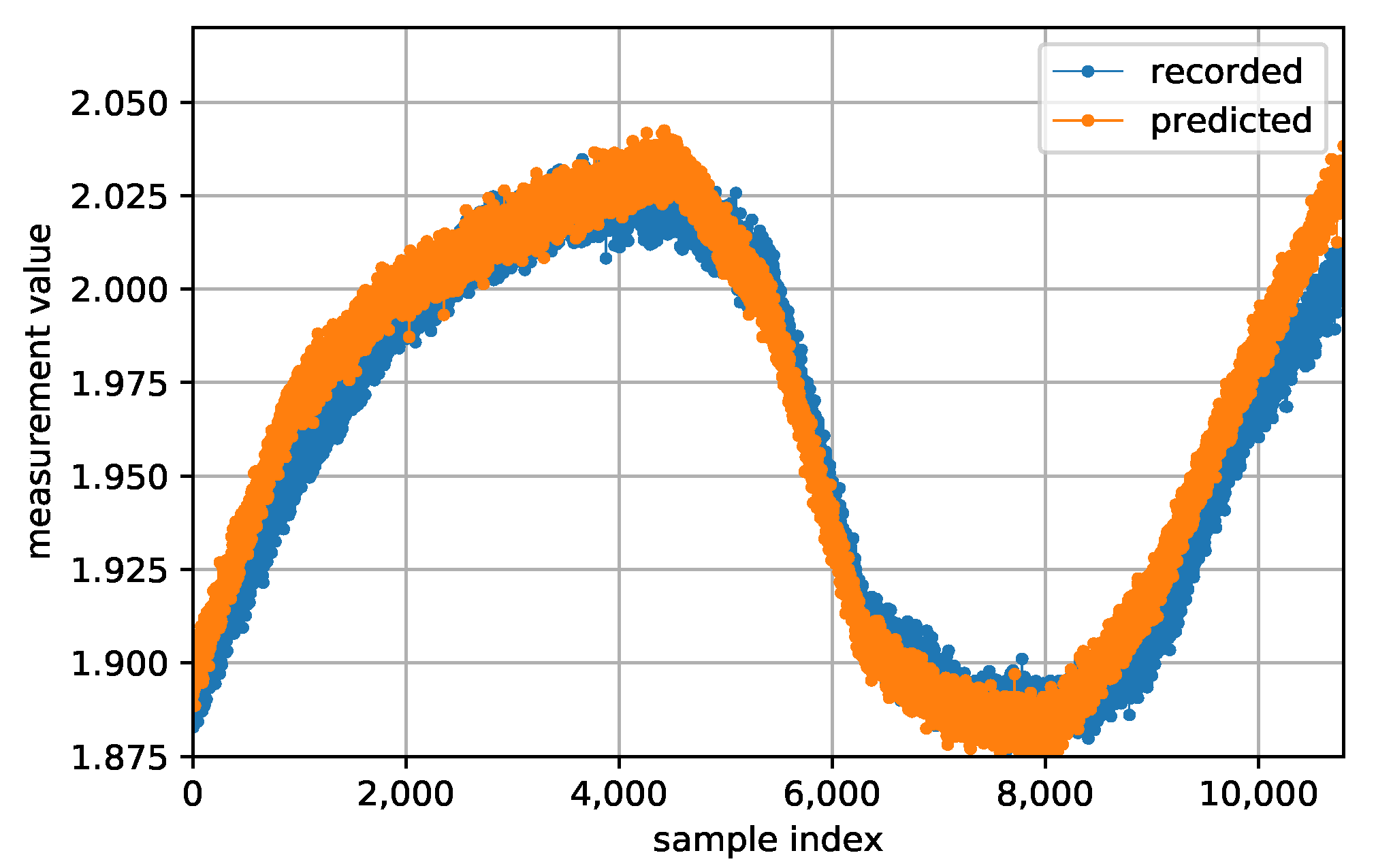
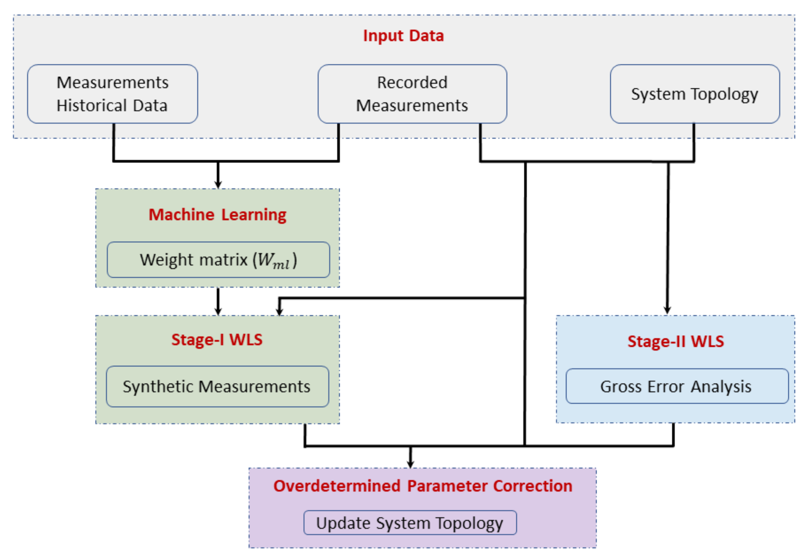
Creating synthetic measurements based on weights obtained from machine learning linear regression prediction;

2.

Developing an overdetermined physics-based model for parameter FDI correction;

3.

Incorporating synthetic measurements in the parameter FDI correction model.

The remainder of this paper is organized as follows. Section 2 provides theoretical background on state estimation with synthetic measurements, the machine learning (ML) model for measurement prediction and the correction model for unbalanced parameter FDI attacks. Section 3 presents the parameter FDI correction physics-based model. Test results of a case study are shown in Section 4. Finally, Section 5 presents conclusions and remarks of this work.

2. Background Information

2.1. State Estimation Augmented with Synthetic Measurements

State estimation aims at solving a set of non-linear algebraic differentiable equations that have the following form [33]:

$$\mathbf{z}=\mathbf{h}\left(\mathbf{x}\right)+\mathbf{e}$$

(1)

where $\mathbf{z}\in {\mathbb{R}}^m$ is the measurement vector, $\mathbf{x}\in {\mathbb{R}}^N$ is the state variables vector, $\mathbf{h}\left(\mathbf{x}\right):{\mathbb{R}}^m\to {\mathbb{R}}^N,(m>N)$ is a non-linear differentiable function that relates the states to the measurements, $\mathbf{e}$ is the measurement error vector assumed with zero mean, standard deviation $\sigma$ and having Gaussian probability distribution, and $N=2n-1$ is the number of unknown state variables. Hence, in the weighted least square state estimation (WLS SE), the approach consists of solving the following minimization problem:

$$\begin{array}{cc}\hfill {\displaystyle \underset{\mathbf{x}}{min}}& \multicolumn{1}{c}{J\left(\mathbf{x}\right)={[\mathbf{z}-\mathbf{h}\left(\mathbf{x}\right)]}^T\mathbf{W}[\mathbf{z}-\mathbf{h}\left(\mathbf{x}\right)]}\end{array}$$

(2)

where $\mathbf{W}$ is a diagonal weight matrix composed by the inverse of the squared values of measurement standard deviations ($\sigma$): $\mathbf{W}$ = $diag\left({[{\sigma }_1^{-2},\dots ,{\sigma }_m^{-2}]}^T\right)$. $J\left(x\right)$ index is a norm in the measurements vector space.

The measurement model in (1) relies on the characterises of the grid, i.e., connectivity and system parameters. If corrupted data is used, then the obtained solution will be physically incorrect, and could potentially mislead the operators who monitor the grid.

In the view of the minimization problem in (2), WLS SE considers minimizing the error as described in (1), which assumes that the residual tends to follow a normal distribution. From the Central Limit Theorem [33], adding large number of independent random variables that follow any distribution with bounded variance, their properly normalized sum tends to approximate a normal distribution. Therefore, for detecting errors using classical WLS, the hypothesis test solely relies on the distribution of ${\chi }^2$. If ${\chi }^2$ distribution does not follow a normal distribution, then the hypotheses test will fail. In ordered to have ${\chi }^2$ distribution to follow a normal distribution the measurement model degrees of freedom needs to be increased. Increasing degree of freedom comes with the financial cost of increasing the measurement set through additional meters.

Ideally, one would want to have a measurement reading in every bus and line section. However, this is not realistic, considering the inherent financial cost. Instead, measurements can be created artificially at locations where no real-life measurement or historical data exist. These measurements, named synthetic measurements, were modeled in [32]. One should not confuse synthetic measurements with pseudo measurements, which are created considering available historical data [33]. The main idea of creating synthetic measurements is to approximate the residual of the measurement model to a normal distribution. In doing so, not only parameter FDI correction is enhanced, as will be presented, but also the global redundancy level of the system increases, which enhances gross error detection and identification [32].

2.2. Linear Regression Prediction Model

Considering a prediction data-driven model selection, performance comparison among several options were made, including linear and non-linear formulations. Test results indicated that a linear regression model was sufficient to yield a great prediction performance. In addition, it is a simpler model with less hyper parameters than other formulations. Multiple linear regression models can be used to estimate SG measurements. The justification for multiple linear regression use is that it is a simple model with few parameters to train. It has been shown that the linear model can achieve satisfying prediction performance on daily load data [29]. Historical measurement values are used as input features to train these multiple linear regression models. During the training, ML model takes historical data (measurement values from past ‘K’ days) as inputs and current day measurements as the target. The training process returns model coefficients that can be used to generate synthetic measurement values from historical measurements. These coefficients estimated using the multiple linear regression model for properly scaled input features also provide an easy way to understand the contribution of each input feature in estimating the target.

Consider D equal to the number of measurement values, and the number of past days used as input features for regression models be K. Thus, D linear regression models can be trained, corresponding to D measurements. The corresponding measurements from K past days are used as input features for the regression model.

$${\mathbf{y}}_d={\mathbf{fi}}_d^0+{\mathbf{fi}}_d^1{\mathbf{x}}_{d1}+\cdots +{\mathbf{fi}}_d^K{\mathbf{x}}_{dK},$$

(3)

where the dependent variable ${\mathbf{y}}_d\in {\mathbb{R}}^{D\times 1}$ is a vector that contains d-th measurement values for the current day, the independent variable ${\mathbf{x}}_{dk}\in {\mathbb{R}}^{D\times 1}$ is a vector that contains d-th measurement values from k-th past day, and ${\mathbf{fi}}_d\in {\mathbb{R}}^{1\times (K+1)}$ is a vector that contains ${\mathbf{fi}}_d^0,{\mathbf{fi}}_d^1,\dots ,{\mathbf{fi}}_d^K$ values.

The regression coefficient matrix $\mathbf{fi}\in {\mathbb{R}}^{D\times (K+1)}$ contains $(K+1)$ values (one for each of the past K days and one intercept) for D multiple linear regression models. $\mathbf{fi}$ is estimated by solving (3) using the Least Squares Fit method. Figure 1 illustrates recorded measurement values and the measurement values prediction by the multiple linear regression models, trained with past temporal data.

We create ‘Weight matrix ($W_{ml}$)’ based on values of regression model coefficients of each measurement. $W_{ml}\in {\mathbb{R}}^{D\times D}$ is used to weigh the measurements in state estimation process and it is calculated from $\mathbf{fi}$ as:

$$W_{ml}^{i,j}=\left\{\begin{array}{cc}\frac{K+1}{{\displaystyle \sum _{k=0}^K}{({\mathbf{fi}}_i^k-\overline{{\mathbf{fi}}_i})}^2},\hfill & \mathrm{if}i=j\hfill \\ 0,\hfill & \mathrm{if}\mathrm{i}\ne \mathrm{j}.\hfill \end{array}\right.$$

(4)

where $i,j=1,2,3,\dots ,D$ represents the measurement number and $\overline{{\mathbf{fi}}_i}$ represents measurement i average of $K+1$ regression coefficients.

As a greater number of days are used to create historical data, the reliance of the model on any one day reduces and the model develops a capability to capture the general measurement deviation patterns. This can improve the generalization ability of the model. We assume that the current day measurements do not deviate from the historical trend by a huge margin and the training data does not have any anomalies. The historical data could be analyzed through bad detection techniques such as [18] for the presence of anomalies and then only the data that does not contain bad data could be used for ML model training.

2.3. Unbalanced Parameter FDI Attack Correction Model

In (1), the possibility of errors in the parameter data is not considered. Instead, if one considers $z=h(x,p)+e$, where p is the parameter in error, this function can be expanded into a Taylor Series [19]:

$$z_i=h_{i,0}+\frac{\partial h_i(x,p)}{\partial p}△p,$$

(5)

where $△p$ denotes the parameter error. From (5), the parameter error can be calculated to be as follow:

$$△p=\frac{z_i-h_{i,0}}{H_{p,0}},$$

(6)

where $H_{p,0}$ denotes the Jacobian of the parameter. All the quantities are known, so the parameter error can be calculated by (6), which is called the relaxed model here, since it considers the measurement without error. With this model, parameter error can be corrected by using measurement value of reactive power flow corresponding to the line where the parameter attack happened through iterations. However, system net parameter values includes three components, which are series conductance g, series susceptance b and shunt susceptance $b^{sh}$. In the meantime, the weights of these three components are decided by network parameter database, so one can only correct the parameter error through this model when these components have the exactly same percentage attack, lets say, $10\%$ on g, $10\%$ on b, and $10\%$ on $b^{sh}$. Thus unbalanced FDI in parameter values are not considered by this model, for example, $30\%$ on g, $20\%$ on b, and $10\%$ on $b^{sh}$. To address this issue, an unbalanced correction model is presented as follows [31]:

$$\left(\begin{array}{c}\Delta g_{km}\\ \Delta b_{km}\\ \Delta b_{km}^{sh}\end{array}\right)={\tau }_n^{-1}\left(\begin{array}{c}{Z}_{P_{k-m\left(loss\right)}}-h_{P_{k-m\left(loss\right)}}^n\\ Z_{P_{k-m}}-h_{P_{k-m}}^n\\ Z_{Q_{k-m}}-h_{Q_{k-m}}^n\end{array}\right),$$

(7)

where the parameter correction Jacobian matrix $\tau$ is defined as:

$$\tau =\left(\begin{array}{ccc}{|E_k-E_m|}^2& 0& 0\\ V_k^2-V_k{V}_{m}cos{\theta }_{km}& -V_k{V}_{m}sin{\theta }_{km}& 0\\ -V_k{V}_{m}sin{\theta }_{km}& -V_k^2+V_k{V}_{m}cos{\theta }_{km}& -V_k^2\end{array}\right).$$

(8)

In (7), n denotes the iteration index; $Z_{P_{k-m\left(loss\right)}}$, $Z_{P_{k-m}}$, $Z_{Q_{k-m}}$ are recorded measurement values of real power loss, real power flow and reactive power flow for FDI attacked line from bus k to m; $h_{P_{k-m\left(loss\right)}}^n$, $h_{P_{k-m}}^n$, $h_{Q_{k-m}}^n$ denote the continuous nonlinear differentiable function of above three quantities at $n_{th}$ iteration. In (8), parameter correction Jacobian matrix $\tau$ uses the magnitude of the voltage drop ${|E_k-E_m|}^2$, voltage injection V and phase difference $\theta$ for bus k and m to perform parameter correction. One can see from (7) and (8), parameter errors of conductance $\Delta g_{km}$, series susceptance $\Delta b_{km}$ and shunt susceptance $\Delta b_{km}^{sh}$ are corrected by using 3 measurements. However, two issues may yield a failure of this process: (1) There are incomplete measurements dataset needed by this model; (2) conductance error $\Delta g_{km}$ can only be estimated from corresponding real power loss measurement which is relatively small in Transmission Line (TL), so an incorrect estimated $\Delta g_{km}$ will cause a wrong estimation of series susceptance error $\Delta b_{km}$ and shunt susceptance error $\Delta b_{km}^{sh}$. To address this issue, a synthetic measurement enhanced parameter correction model is presented in this paper.

3. Synthetic Measurement Enhanced Parameter Error Correction

3.1. Framework for Parameter FDI Correction

The parameter FDI correction framework is illustrated in Figure 2. Input data consists of historical measurements of the system for the past days, recorded measurements from meters, parameters data and system topology such as connectivity status. The Machine Learning (ML) model process measurements from past days to predict measurements of the current day. The resultant weights attained from ML model are considered in stage—I WLS state estimation, which generates SM. Meanwhile, gross error analysis is performed in stage—II WLS state estimation. In this stage, FDI detection and identification is taken place [18,19]. Upon detecting and identifying parameter attacks in the network, a parameter FDI correction model is solved. Once parameter correction performed, system model is updated.

The process of creating SM is referred to as stage—I WLS in Figure 2. In this stage, existing measurements (bus power injection, power flow and voltage measurements) are weighted based on weights derived from ML models described in Section 2.2. Upon WLS SE convergence, power flow estimates in lines with no real-life measurement recorded are to be used as SM. The idea here is to increase, artificially, local measurement redundancy, with linear independent information, providing thus the necessary condition for the development of an overdetermined database of network parameters FDI cyber attack correction model. Hence, for every line section, there will be power flow measurement reading from both ends of the lines. These SM in addition to existing scan of measurements are processed in the FDI correction model, described in Section 3.2.

3.2. Overdetermined Parameter FDI Correction Model

Consider the conjugate of the complex power flow [33]:

$$\begin{array}{cc}\hfill S_{k-m}^{*}& =E_k^{*}{I}_{k-m}\hfill \\ & =y_{k-m}{V}_k{e}^{-j{\theta }_k}(V_k{e}^{j{\theta }_k}-V_m{e}^{j{\theta }_m})+j{b}_{km}^{sh}{V}_k^2.\hfill \end{array}$$

(9)

The expressions for real and reactive power flows can be obtained by identifying the corresponding coefficients of the real and the imaginary parts of (9):

$$\begin{array}{c}\hfill P_{k-m}=V_k^2{g}_{km}-V_k{V}_m{g}_{km}\cos {\theta }_{km}\\ \hfill -V_k{V}_m{b}_{km}\sin {\theta }_{km},\end{array}$$

(10)

$$\begin{array}{c}\hfill Q_{k-m}=-V_k^2(b_{km}+b_{km}^{sh})+V_k{V}_m{b}_{km}cos{\theta }_{km}\\ \hfill -V_k{V}_m{g}_{km}sin{\theta }_{km}.\end{array}$$

(11)

Through equation (10), one can derive the real power loss of a line:

$$\begin{array}{cc}\hfill P_{k-m\left(loss\right)}& =P_{k-m}+P_{m-k}\hfill \\ & =g_{km}(V_k^2+V_m^2-2V_k{V}_{m}cos{\theta }_{km})\hfill \\ & =g_{km}{|E_k-E_m|}^2,\hfill \end{array}$$

(12)

Through equation (11), one can derive the reactive power loss of a line:

$$\begin{array}{cc}\hfill Q_{k-m\left(loss\right)}& =Q_{k-m}+Q_{m-k}\hfill \\ & =-b_{km}^{sh}(V_k^2+V_m^2)\hfill \\ & -b_{km}(V_k^2+V_m^2-2V_k{V}_{m}cos{\theta }_{km})\hfill \\ & =-b_{km}^{sh}(V_k^2+V_m^2)-b_{km}{|E_k-E_m|}^2.\hfill \end{array}$$

(13)

Equations (10)–(13) provide a model which correlates the real power flow losses, reactive power losses, real power flow, and reactive power flow with system net parameters, as (14) and (15). It is important to note that in this framework, all six of the measurements in (14) are always used in the correction process, but they may not all be real measurements. Any measurements that are not available through a sensor are calculated as SM as described earlier. For example, if the $P_{k-m}$, and $Q_{k-m}$ are the only true measurements, $P_{m-k}$, and $Q_{m-k}$ will be SM. $P_{k-m\left(loss\right)}$ will be calculated by $P_{k-m}$ and $P_{m-k}$, $Q_{k-m\left(loss\right)}$ will be obtained by $Q_{k-m}$ and $Q_{m-k}$.

$$\begin{array}{c}\hfill {\tau }_{up}\left(\begin{array}{c}{g}_{km}\\ b_{km}\\ b_{km}^{sh}\end{array}\right)=\left(\begin{array}{c}{P}_{k-m\left(loss\right)}\\ Q_{k-m\left(loss\right)}\\ P_{k-m}\\ P_{m-k}\\ Q_{k-m}\\ Q_{m-k}\end{array}\right),\end{array}$$

(14)

where ${\tau }_{up}$ is defined as:

$${\tau }_{up}=\left(\begin{array}{ccc}{|E_k-E_m|}^2& 0& 0\\ 0& -{|E_k-E_m|}^2& -(V_k^2+V_m^2)\\ V_k^2-V_k{V}_{m}cos{\theta }_{km}& -V_k{V}_{m}sin{\theta }_{km}& 0\\ V_m^2-V_k{V}_{m}cos{\theta }_{km}& V_k{V}_{m}sin{\theta }_{km}& 0\\ -V_k{V}_{m}sin{\theta }_{km}& -V_k^2+V_k{V}_{m}cos{\theta }_{km}& -V_k^2\\ V_k{V}_{m}sin{\theta }_{km}& -V_m^2+V_k{V}_{m}cos{\theta }_{km}& -V_m^2\end{array}\right)$$

(15)

By linearizing (14) through a Taylor series, considering a Newton-Raphson method at $n^{th}$ iteration:

$$\begin{array}{c}\hfill {\tau }_{{up}_n}\left(\begin{array}{c}\Delta g_{km}\\ \Delta b_{km}\\ \Delta b_{km}^{sh}\end{array}\right)=A\end{array},$$

(16)

where A is the residual of the set of measurements associated with the correction of line parameters as follows:

$$\begin{array}{c}\hfill A=\left(\begin{array}{c}{Z}_{P_{k-m\left(loss\right)}}-h_{P_{k-m\left(loss\right)}}^n\\ Z_{Q_{k-m\left(loss\right)}}-h_{Q_{k-m\left(loss\right)}}^n\\ Z_{P_{k-m}}-h_{P_{k-m}}^n\\ Z_{P_{m-k}}-h_{P_{m-k}}^n\\ Z_{Q_{k-m}}-h_{Q_{k-m}}^n\\ Z_{Q_{m-k}}-h_{Q_{m-k}}^n\end{array}\right)\end{array}.$$

(17)

The expression in (15) shows that augmenting ${\tau }_{up}$ and the measurements set, will change the model in (8) into an overdetermined system of nonlinear algebraic equations. Model (16) can be solved considering the minimization problem:

$$\underset{\Delta g_{km},\Delta b_{km},\Delta b_{km}^{sh}}{min}{[{\tau }_{up}\left(\begin{array}{c}\Delta g_{km}\\ \Delta b_{km}\\ \Delta b_{km}^{sh}\end{array}\right)-A]}^T{W}_p[{\tau }_{up}\left(\begin{array}{c}\Delta g_{km}\\ \Delta b_{km}\\ \Delta b_{km}^{sh}\end{array}\right)-A].$$

(18)

One finds the classical WLS SE solution for (18) is:

$$\left(\begin{array}{c}\Delta g_{km}\\ \Delta b_{km}\\ \Delta b_{km}^{sh}\end{array}\right)={\left({\tau }_{up}^T{W}_p{\tau }_{up}\right)}^{-1}{\tau }_{up}^T{W}_{p}A,$$

(19)

where $W_p$ is the weight matrix for parameter correction, ${\sigma }_r$ in each element denotes one standard deviation of corresponding residue at each iteration:

$$W_p=diag\left([\frac{1}{{\sigma }_{r_{P_{k-m\left(loss\right)}}}^2},\frac{1}{{\sigma }_{r_{Q_{k-m\left(loss\right)}}}^2},\dots ,\frac{1}{{\sigma }_{r_{Q_{m-k}}}^2}]\right).$$

(20)

4. Case Study

The presented model is validated using the IEEE 118-bus system. Topology and parameters of the IEEE 118-bus system are found in [34]. With the aid of MATPOWER [35], a measurement set is obtained, which consists of 712 measurement leading to a global redundancy level (GRL) 3.029. A Gaussian noise with zero mean and known variance is added to the measurement set. In addition, a measurement dataset corresponding to eight consecutive days each of which one contains 21,600 samples based on a common daily load profile that contains temporal information of a power system’s changing state is generated and fed to machine learning models for measurements prediction and measurements’ weight. It is worth noting that different noise levels were used for generating multiple datasets. Real line power flows, reactive line power flows, bus power injections, and voltage magnitudes are included in each measurement set. The implementation and evaluation of the machine learning algorithm was executed using python libraries such as NumPy [36], SciPy [37], Matplotlib [38] and Scikit-learn [39]. The first $50\%$ of the samples in each day are used to train multiple linear regression models.

In the following, two different parameter FDI attack scenarios are presented. In each scenario, attack detection is flagged if the objective function $J\left(x\right)$ is above threshold value $C={\chi }_{p,dof}^2$. Identification is performed by building a descending list of $CM{E}^N$ (based on their absolute values) [19]. In the correction step, the presented model in Section 2.1 is solved.

4.1. Parameter Attack Scenario I

In scenario I, an unbalanced parameter FDI attack is injected to the series and shunt parameter of the line 23–32 ($-18\%$ on parameter g, $12\%$ on parameter b, $-6\%$ on parameter $b^{sh}$) on the IEEE 118-bus system.

In this case, the parameters of line 23–32 are attacked. The first process of the framework is FDI detection. Results are presented in

Table 1. Processing cyber-attacks.

Processing Measurement Cyber-Attack Step 1
J (x) = 1246.587 > C = 775.1861 Attack Detected!
${\mathit{CME}}^{\mathit{N}}$Descending List
Measurement	$\mathit{II}$	${\mathit{CME}}^{\mathit{N}}$
$Q_{23}$	0.0395	−8.4156
$Q_{32–23}$	3.9464	6.9948
$Q_{23–25}$	0.1380	5.9432
$P_{23–32}$	0.3557	5.5826
$Q_{24}$	0.4774	−4.4724
$Q_{32}$	3.9464	3.9948

. One can see that the objective function $J\left(x\right)$ is 1246.587, which is higher than threshold value (C = ${\chi }^2$ = 775.1861), thus a cyber attack is detected. For identification, a descending list of $CM{E}^N$ is built. From the resultant list, the largest absolute value of $CM{E}^N$ which is 8.4156 is related to reactive power injection for bus 23. In addition, one can see that the $CM{E}^N$ value of corresponding reactive power flow $Q_{32–23}$, real power flow $P_{23–32}$ and reactive power injection $Q_{32}$ are also above the threshold value ($\beta =3$). This situation is characterized as a parameter attack on line 23–32 [19]. For parameter correction, the process described in Section 2.1 is implemented. The results are shown in

Table 2. Corrected Parameters using the updated parameter correction Jacobian matrix ${\tau }_{up}$.

Parameter Correction
Parameter	Database	Erroneous	Presented Correction (Approximation Error)	State-of-the-Art Correction (Approximation Error) [31]
$g_{23–32}$	2.2169	1.8179	2.2285 $(0.525\%)$	2.2385 $(0.974\%)$
$b_{23–32}$	−8.0635	−9.0311	−8.0782 $(0.183\%)$	−8.0854 $(0.271\%)$
$b_{23–32}^{sh}$	0.0587	0.0551	0.0586$(0.170\%)$	0.0589$(0.340\%)$

. In the state of the art parameter correction model [31] (also presented in (7)), one can clearly see that the model requires at least three different real-life measurements: two real power flow $P_{km}$, $P_{mk}$ and one reactive power flow measurement $Q_{km}$. However, there is no guarantee that the required measurements will exist. For example, in the current testing measurement configuration, only 1 real power flow $P_{23–32}$ measurement and 1 reactive power flow $Q_{32–23}$ measurement are assumed to exist. Therefore, the correction model in (7) is unable to process the expecting correction due to the unavailability of the power flow measurement $P_{32–23}$. To resolve this issue, in the presented framework, synthetic measurements are considered only for unavailable measurements. These synthetic measurements are generated by running WLS SE using weights obtained from machine learning linear regression prediction. For this task, no gross error detection analytics is performed. In this case, 358 SMs are generated (adding 358 SM yields a GRL increase from 3.029 to 4.55). Then, two synthetic measurements $P_{32–23}$ and $Q_{23–32}$ are obtained and augmented from SM dataset. Parameter correction is processed by using 2 existing measurements and two synthetic measurements in the presented parameter FDI correction model (18). Results of such correction are presented in Figure 3. As one can see, the parameter correction process converges at 26th iteration while approximation errors for $g_{23–32}$, $b_{23–32}$, $b_{23–32}^{sh}$ are $(0.525\%)$, $(0.183\%)$, $(0.340\%)$ respectively, which are all lower than state of the art model in [31]. After parameter correction is obtained, a new state estimation process is performed in which objective function $J\left(x\right)$ is found to be 684.5437, which is lower than threshold value C. Hence, no FDI attack is detected.

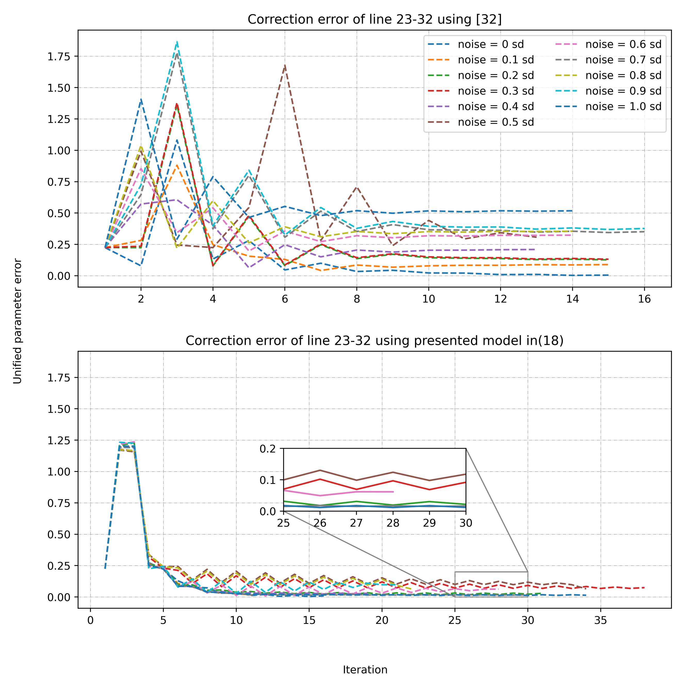
4.2. Parameter Attack Scenario II

• A measurement cyber-attack of magnitude 5 $\sigma$ is added to reactive power flow from bus 31 to bus 17 ($Q_{31–17}$).
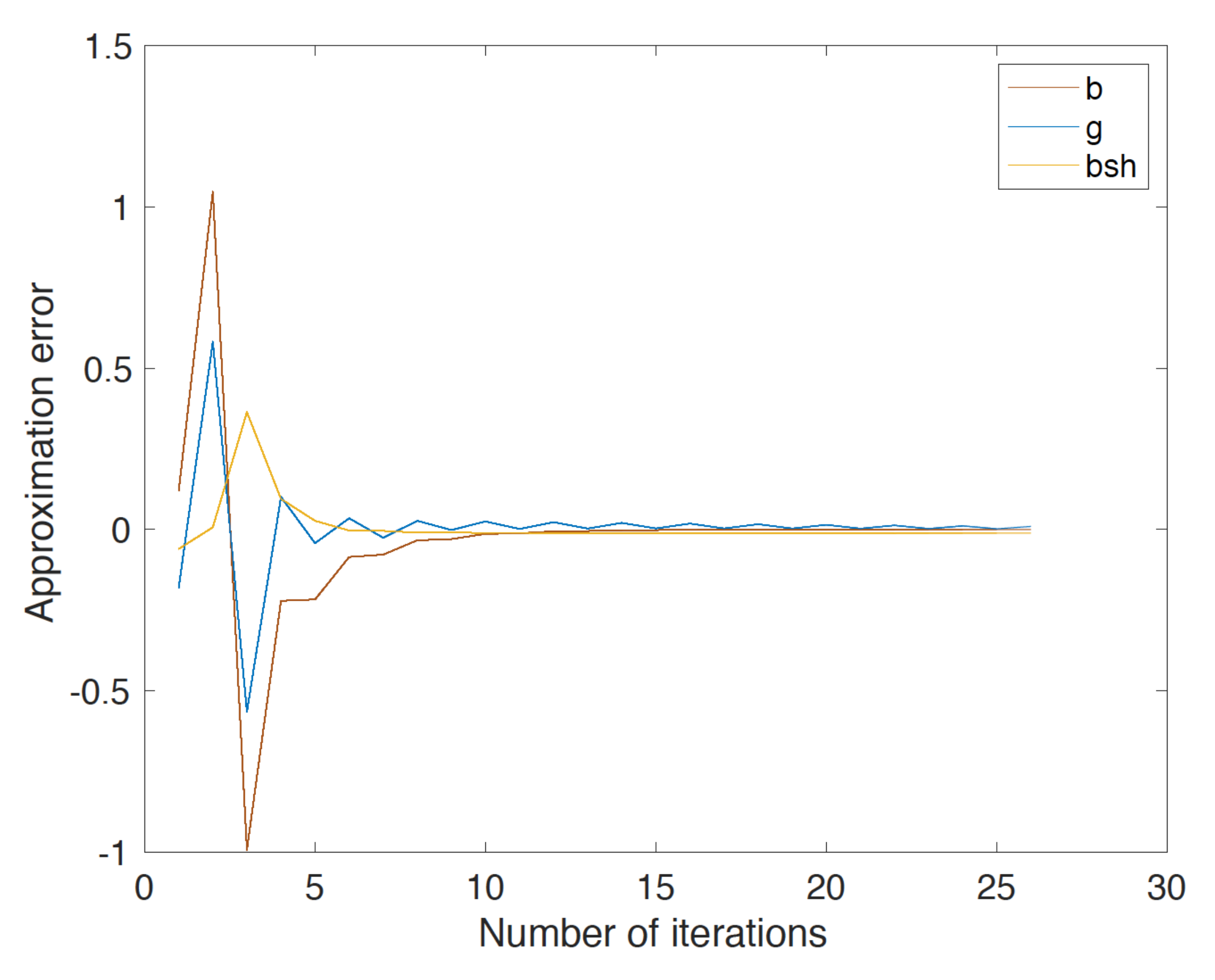
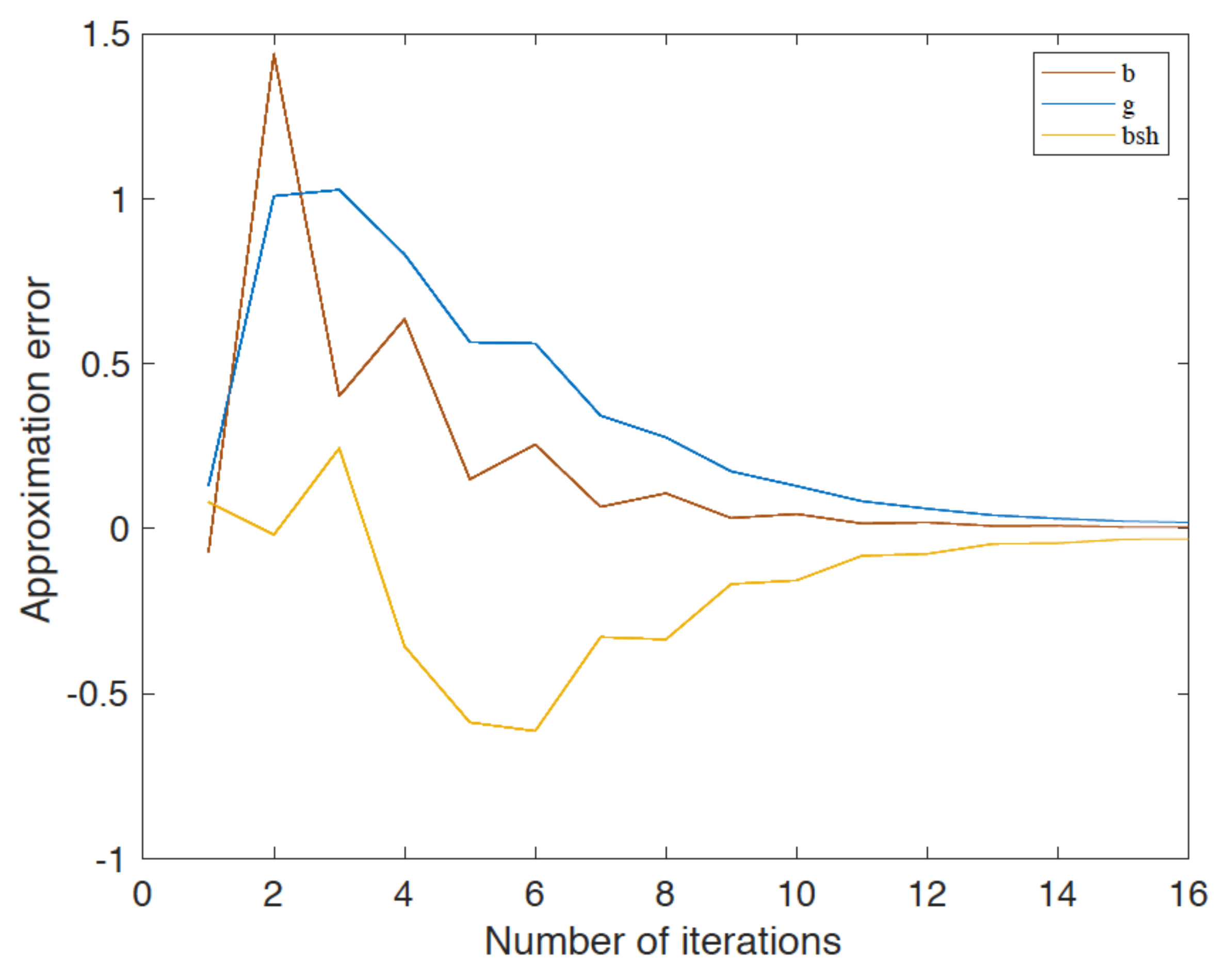
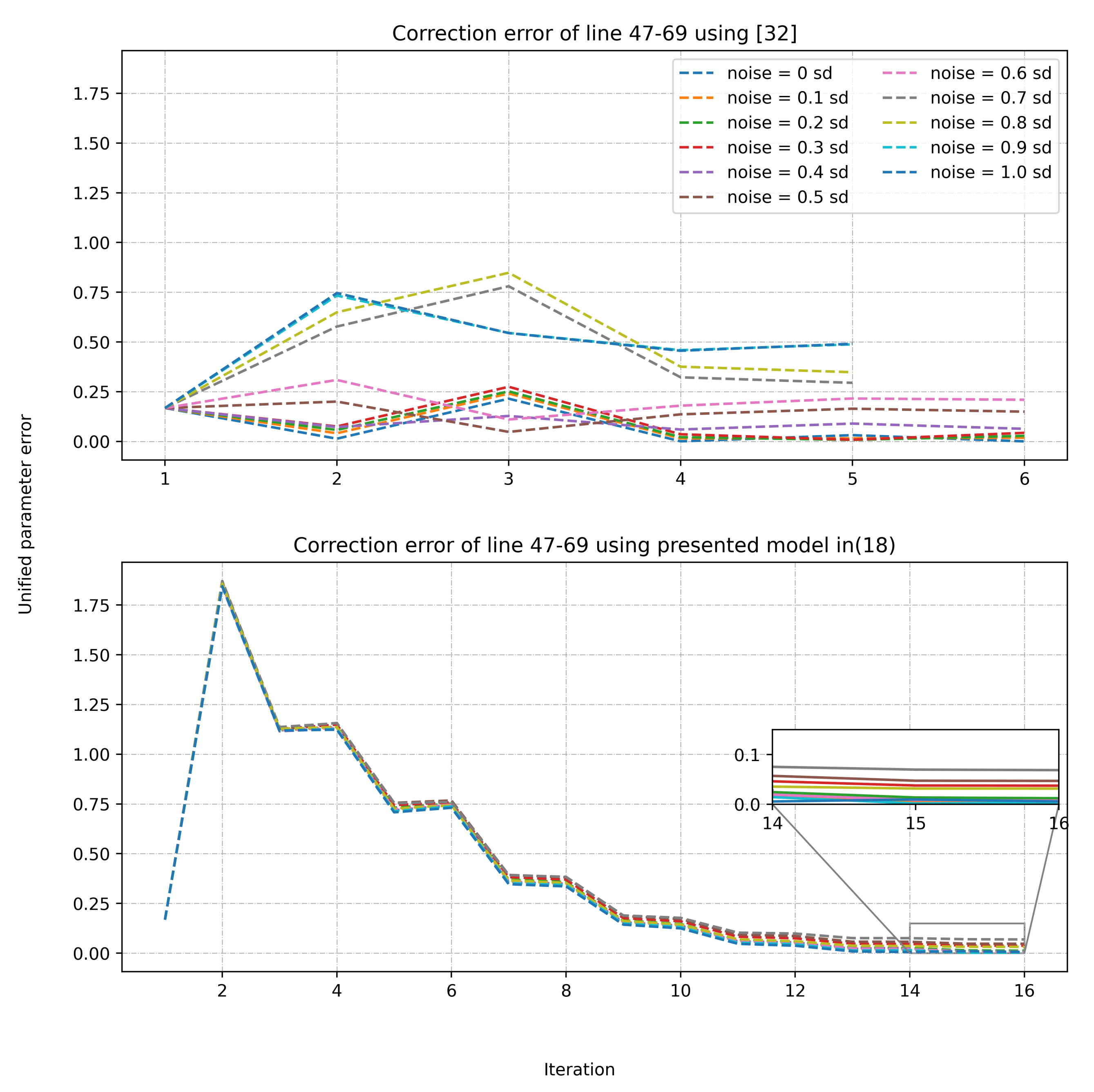
• An unbalanced parameter FDI attack is injected to the series and shunt parameter of the line 47–69 ($13\%$ on parameter g, $-7\%$ on parameter b, $8\%$ on parameter $b^{sh}$).

In this scenario, the attack is detected and the result is shown in

Table 3. Processing Cyber-attacks.

Processing Measurement Cyber-Attack Step 1
J (x) = 1133.8323 > C = 775.1861 Attack Detected!
${\mathit{CME}}^{\mathit{N}}$ Descending List
Measurement	$\mathit{II}$	${\mathit{CME}}^{\mathit{N}}$
$Q_{47}$	1.9344	15.6324
$P_{47}$	0.2513	9.2054
$P_{69–47}$	4.8151	−7.8438
$Q_{69–47}$	6.0617	−7.6539
$P_{46}$	0.3380	6.2045
$Q_{31–17}$	2.8898	5.6933
$P_{45–46}$	6.6911	4.2257

, where the objective function is higher than the C value for this scenario ($C={\chi }^2=775.1861$). For identification step, a descending list of $CM{E}^N$ is built and shown in the same table. The largest $CM{E}^N$ values (absolute values) are associated with reactive power injection $Q_{47}$, real power injection $P_{47}$, real power flow $P_{69–47}$ and reactive power flow $Q_{69–47}$. This scenario characterizes a parameter cyber-attack on line 47–69 [19]. After identification, the net system parameter are corrected using the presented model in (18). Still, only flow $P_{69–47}$ and $Q_{69–47}$ are provided in current measurements configuration. The lack of missing the real power flow measurement $P_{47–69}$ limits the possibility of performing state of the art model in (7), since incomplete information prevent this model to calculate real power loss mentioned in (7). However, with synthetic measurement $Q_{47–69}$ and $P_{47–69}$ provided, one will be able to use presented overdetermined model in (18) to perform parameter correction. Correction converges after 16 iterations, and corrected values and comparable results are presented in

Table 4. Corrected parameters using the updated parameter correction Jacobian matrix ${\tau }_{up}$.

Parameter Correction
Parameter	Database	Erroneous	Presented Correction (Approximation Error)	State-of-the-art Correction (Approximation Error) [31]
$g_{47–69}$	1.0012	1.1314	1.0062 $(0.499\%)$	1.0088 $(0.759\%)$
$b_{47–69}$	−3.2955	−3.0648	−3.2876 $(0.241\%)$	−3.2826 $(0.361\%)$
$b_{47–69}^{sh}$	0.0355	0.0383	0.035532$(0.092\%)$	0.0357$(0.563\%)$

. System net parameters $g_{47–69}$, $b_{47–69}$, $b_{47–69}^{sh}$ have approximation error $(0.499\%)$, $(0.241\%)$ and $(0.092\%)$ after convergence. After correction, a new state estimation is performed, objective function value 837.6015 is obtained which is still higher than threshold C in

Table 5. Processing Cyber-attacks.

Processing Measurement Cyber-Attack Step 1
$\mathit{J}\left(\mathit{x}\right)=\mathbf{837}.\mathbf{6015}>\mathbf{C}=\mathbf{775}.\mathbf{1861}$ Attack Detected!
${\mathit{CME}}^{\mathit{N}}$ Descending List
Measurement	$\mathit{II}$	${\mathit{CME}}^{\mathit{N}}$	$\mathit{CNE}$
$Q_{31–17}$	2.8541	5.2318	5.2044

. As seen, the only $CM{E}^N$ value (absolute value) above the threshold is the reactive power flow $Q_{31–17}$. Therefore, the measurement $Q_{31–17}$ is in error. The correction of measurements as shown in the flowchart is performed using their $CNE$ values. The corrected measurement is shown in

Table 6. Corrected measurement using the CNE.

Measurement Correction
Measurement	Database	Erroneous	Correction Using CNE (Approximation Error) [30]
$Q_{31–17}$	−0.1754	−0.1643	−0.1761 $(0.399\%)$

. After re-running the state estimator, the ${\chi }^2$ is smaller than C, thus no further FDI attack detected.

To further evaluate the robustness of presented model, different measurement noise levels are simulated. A combined parameter error metric is presented to illustrate the total parameter error after correction, while $\Vert e^p=\frac{[g_{km};b_{km};b_{km}^{sh}]-[g_{km}\left(base\right);b_{km}\left(base\right);b_{km}^{sh}\left(base\right)]}{[g_{km}\left(base\right);b_{km}\left(base\right);b_{km}^{sh}\left(base\right)]}{\Vert }_2$. $e^p$ represents the weighted norm of the sum of all parameter errors. A 100 Monte-Carlo simulation is performed and average value is presented. Figure 4 shows a comparison between state-of-the-art solution presented in (7) and proposed model (18). One can see in Figure 5 that the error increases with noise level when using state-of-the-art solution model. However, the proposed model under different noise level provides error below 0.07.

To further illustrate the robustness of proposed solution under different noise level, comparison result is presented in Figure 6. In Figure 6, the highest error $e^p$ of line 47–69 reaches 0.5 after system convergence when the noise level increase to 1 standard deviation using state-of-the-art solution (7), while using presented model (18) all values of $e^p$, under different noise level, are lower than 0.06.

5. Conclusions

In this paper, a physics-based model for malicious parameter FDI cyber-attacks correction is presented. An FDI framework is further presented to detect, identify and correct FDI attacks on measurements and database of the network parameters. The main foundation of the proposed framework relies on creating synthetic measurements that are derived based on weights obtained from linear regression measurement prediction. Synthetic measurements, in addition to recorded measurements, are used in an overdetermined parameter correction model to estimate and correct network parameters. Simulation results show that the presented framework is able to obtain parameter approximation error less than $1\%$ under different noise level from 0 to 1% standard deviation, which outperforms state of the art solution. In addition to the robustness of the presented model, the framework can be easily integrated, without hard-to-design parameters, to the classical WLS SE software, which highlights potential aspects for real-life implementation.

References

1. Farag, M.; Azab, M.; Mokhtar, B. Cross-Layer Security Framework for Smart Grid: Physical Security Layer. In Proceedings of the IEEE PES Innovative Smart Grid Technologies Europe (ISGT Europe), Istanbul, Turkey, 12–15 October 2014; pp. 1–7. [Google Scholar]
2. Stefanov, A.; Liu, C. Cyber-power system security in a smart grid environment. In Proceedings of the 2012 IEEE PES Innovative Smart Grid Technologies (ISGT), Washington, DC, USA, 16–20 January 2012; pp. 1–3. [Google Scholar] [CrossRef]
3. Liu, Y.; Ning, P.; Reiter, M.K. False data injection attacks against state estimation in electric power grids. ACM Trans. Inf. Syst. Secur. TISSEC 2011, 14, 13. [Google Scholar] [CrossRef]
4. Kosut, O.; Jia, L.; Thomas, R.J.; Tong, L. Malicious data attacks on the smart grid. IEEE Trans. Smart Grid 2011, 2, 645–658. [Google Scholar] [CrossRef] [Green Version]
5. Bi, S.; Zhang, Y.J.A. Graph-based Cyber Security Analysis of State Estimation in Smart Power Grid. IEEE Commun. Mag. 2017, 55, 176–183. [Google Scholar] [CrossRef]
6. Li, S.; Yılmaz, Y.; Wang, X. Quickest detection of false data injection attack in wide-area smart grids. IEEE Trans. Smart Grid 2015, 6, 2725–2735. [Google Scholar] [CrossRef]
7. Li, S.; Yilmaz, Y.; Wang, X. Sequential cyber-attack detection in the large-scale smart grid system. In Proceedings of the 2015 IEEE International Conference on Smart Grid Communications (SmartGridComm), Miami, FL, USA, 2–5 November 2015; pp. 127–132. [Google Scholar]
8. Volz, D. U.S. government concludes cyber attack caused Ukraine power outage. Reuters, 25 February 2016. [Google Scholar]
9. Wang, Y.; Xia, M.; Chen, Q.; Chen, F.; Yang, X.; Han, F. Fast State Estimation of Power System based on Extreme Learning Machine Pseudo-Measurement Modeling. In Proceedings of the 2019 IEEE Innovative Smart Grid Technologies—Asia (ISGT Asia), Chengdu, China, 21–24 May 2019; pp. 1236–1241. [Google Scholar]
10. Chakhchoukh, Y.; Liu, S.; Sugiyama, M.; Ishii, H. Statistical outlier detection for diagnosis of cyber attacks in power state estimation. In Proceedings of the 2016 IEEE Power and Energy Society General Meeting (PESGM), Boston, MA, USA, 17–21 July 2016; pp. 1–5. [Google Scholar]
11. Ahmed, S.; Lee, Y.; Hyun, S.; Koo, I. Feature Selection–Based Detection of Covert Cyber Deception Assaults in Smart Grid Communications Networks Using Machine Learning. IEEE Access 2018, 6, 27518–27529. [Google Scholar] [CrossRef]
12. Zou, T.; Aljohani, N.; Wang, P.; Bretas, A.S.; Bretas, N.G. Distributed nonlinear state estimation using adaptive penalty parameters with load characteristics in the Electricity Reliability Council of Texas. J. Ind. Inf. Integr. 2021, 24, 100223. [Google Scholar]
13. Panthi, M. Anomaly Detection in Smart Grids using Machine Learning Techniques. In Proceedings of the 2020 First International Conference on Power, Control and Computing Technologies (ICPC2T), Raipur, India, 3–5 January 2020; pp. 220–222. [Google Scholar]
14. Cao, J.; Wang, D.; Qu, Z.; Cui, M.; Xu, P.; Xue, K.; Hu, K. A Novel False Data Injection Attack Detection Model of the Cyber-Physical Power System. IEEE Access 2020, 8, 95109–95125. [Google Scholar] [CrossRef]
15. Zonouz, S.A.; Rogers, K.M.; Berthier, R.; Bobba, R.; Sanders, W.H.; Overbye, T.J. SCPSE: Security-Oriented Cyber-Physical State Estimation for Power Grid Critical Infrastructures. IEEE Trans. Smart Grid 2012, 3, 1790–1799. [Google Scholar] [CrossRef]
16. Sridhar, S.; Govindarasu, M. Model-Based Attack Detection and Mitigation for Automatic Generation Control. IEEE Trans. Smart Grid 2014, 5, 580–591. [Google Scholar] [CrossRef]
17. Trevizan, R.D.; Ruben, C.; Nagaraj, K.; Ibukun, L.L.; Starke, A.C.; Bretas, A.S.; McNair, J.; Zare, A. Data-driven Physics-based Solution for False Data Injection Diagnosis in Smart Grids. In Proceedings of the 2019 IEEE PES GM, Atlanta, GA, USA, 4–8 August 2019. [Google Scholar]
18. Nagaraj, K.; Zou, S.; Ruben, C.; Dhulipala, S.C.; Starke, A.; Bretas, A.; Zare, A.; McNair, J. Ensemble CorrDet with Adaptive Statistics for Bad Data Detection. IET Smart Grid 2020, 3, 572–580. [Google Scholar] [CrossRef]
19. Bretas, A.S.; Bretas, N.G.; Carvalho, B.E. Further contributions to smart grids cyber-physical security as a malicious data attack: Proof and properties of the parameter error spreading out to the measurements and a relaxed correction model. Int. J. Electr. Power Energy Syst. 2019, 104, 43–51. [Google Scholar] [CrossRef]
20. Liu, C.; Liang, H.; Chen, T. Network Parameter Coordinated False Data Injection Attacks against Power System AC State Estimation. IEEE Trans. Smart Grid 2020. [Google Scholar] [CrossRef]
21. Abur, A.; Expósito, A. Power System State Estimation: Theory and Implementation; Power Engineering (Willis); CRC Press: Boca Raton, FL, USA, 2004. [Google Scholar]
22. Abur, A.; Zhu, J. Identification of parameter errors. In Proceedings of the IEEE PES General Meeting, Detroit, MI, USA, 24–28 July 2010; pp. 1–4.
23. Lin, Y.; Abur, A. Fast Correction of Network Parameter Errors. IEEE Trans. Power Syst. 2018, 33, 1095–1096. [Google Scholar] [CrossRef]
24. Carvalho, B.; Bretas, N.; Bretas, A. A local state vector augmentation technique for processing network parameters errors. In Proceedings of the 2017 IEEE Power Energy Society General Meeting, Chicago, IL, USA, 16–20 July 2017; pp. 1–5. [Google Scholar]
25. Wang, Q.; Tai, W.; Tang, Y.; Ni, M.; You, S. A two-layer game theoretical attack-defense model for a false data injection attack against power systems. Int. J. Electr. Power Energy Syst. 2019, 104, 169–177. [Google Scholar] [CrossRef]
26. Bansal, P.; Singh, A. Smart metering in smart grid framework: A review. In Proceedings of the 2016 Fourth International Conference on Parallel, Distributed and Grid Computing (PDGC), Waknaghat, India, 22–24 December 2016; pp. 174–176. [Google Scholar]
27. Bretas, A.S.; Bretas, N.G.; Carvalho, B.; Baeyens, E.; Khargonekar, P.P. Smart grids cyber-physical security as a malicious data attack: An innovation approach. Electr. Power Syst. Res. 2017, 149, 210–219. [Google Scholar] [CrossRef]
28. Zou, T.; Bretas, A.S.; Aljohani, N.; Bretas, N.G. Malicious data injection attacks: A relaxed physics model based strategy for real-time monitoring. In Proceedings of the 2019 North American Power Symposium (NAPS), Wichita, KS, USA, 13–15 October 2019; pp. 1–6. [Google Scholar]
29. Nagaraj, K.; Aljohani, N.; Zou, S.; Ruben, C.; Bretas, A.; Zare, A.; McNair, J. State Estimator and Machine Learning Analysis of Residual Differences to Detect and Identify FDI and Parameter Errors in Smart Grids. In Proceedings of the 2020 North American Power Symposium (NAPS), Tempe, AZ, USA, 11–13 April 2020; pp. 1–6. [Google Scholar]
30. Bretas, N.G.; Bretas, A.S. The extension of the Gauss approach for the solution of an overdetermined set of algebraic non linear equations. IEEE Trans. Circuits Syst. II Express Briefs 2018, 65, 1269–1273. [Google Scholar] [CrossRef]
31. Zou, T.; Bretas, A.S.; Ruben, C.; Dhulipala, S.C.; Bretas, N. Smart grids cyber-physical security: Parameter correction model against unbalanced false data injection attacks. Electr. Power Syst. Res. 2020, 187, 106490. [Google Scholar] [CrossRef]
32. Bretas, A.S.; Rossoni, A.; Trevizan, R.D.; Bretas, N.G. Distribution networks nontechnical power loss estimation: A hybrid data-driven physics model-based framework. Electr. Power Syst. Res. 2020, 186, 106397. [Google Scholar] [CrossRef]
33. Bretas, A.S.; Bretas, N.G.; London, J.B.; Carvalho, B.E. Cyber-Physical Power Systems State Estimation; Elsevier: Amsterdam, The Netherlands, 2021. [Google Scholar]
34. Christie, R. Power Systems Test Case Archive; Electrical Engineering Department, University of Washington: Washington, DC, USA, 2000. [Google Scholar]
35. Zimmerman, R.D.; Murillo-Sanchez, C.E.; Thomas, R.J. MATPOWER: Steady-State Operations, Planning, and Analysis Tools for Power Systems Research and Education. IEEE Trans. Power Syst. 2011, 26, 12–19. [Google Scholar] [CrossRef] [Green Version]
36. Oliphant, T.E. A Guide to NumPy; 2006; Volume 1, Available online: https://ecs.wgtn.ac.nz/foswiki/pub/Support/ManualPagesAndDocumentation/numpybook.pdf (accessed on 26 August 2021).
37. Virtanen, P.; Gommers, R.; Oliphant, T.E.; Contributors, S. SciPy 1.0: Fundamental Algorithms for Scientific Computing in Python. Nat. Methods 2020, 17, 261–272. [Google Scholar] [CrossRef] [Green Version]
38. Hunter, J.D. Matplotlib: A 2D graphics environment. Comput. Sci. Eng. 2007, 9, 90–95. [Google Scholar] [CrossRef]
39. Pedregosa, F.; Varoquaux, G.; Gramfort, A.; Michel, V.; Thirion, B.; Grisel, O.; Blondel, M.; Prettenhofer, P.; Weiss, R.; Dubourg, V.; et al. Scikit-learn: Machine Learning in Python. J. Mach. Learn. Res. 2011, 12, 2825–2830. [Google Scholar]
Figure 1. An example for ML-predicted measurement vs. recorded measurement value.
Applsci 11 08074 g001
Figure 2. Framework for parameter FDI correction.
Applsci 11 08074 g002
Figure 3. Correction for line 23–32 using presented model (18).
Applsci 11 08074 g003
Figure 4. Correction for line 47–69 using presented model (18).
Applsci 11 08074 g004
Figure 5. Correction for line 23–32.
Applsci 11 08074 g005
Figure 6. Correction for line 47–69.
Applsci 11 08074 g006