Optical Classification of Lower Amazon Waters Based on In Situ Data and Sentinel-3 Ocean and Land Color Instrument Imagery

Abstract

Optical water types (OWTs) were identified from an in situ dataset of concomitant biogeochemical and optical parameters acquired in the Amazon River and its tributaries, in the Lower Amazon region, at different hydrological conditions from 2014 to 2017. A seasonal bio-optical characterization was performed. The k-means classification was applied to the in situ normalized reflectance spectra ($r_n\left(\lambda \right)$), allowing the identification of four OWTs. An optical index method was also applied to the $r_n\left(\lambda \right)$ defining the thresholds of the OWTs. Next, level-3 Sentinel-3 Ocean and Land Color Instrument images representative of the seasonal discharge conditions were classified using the identified in situ OWTs as reference. The differences between Amazon River and clearwater tributary OWTs were dependent on the hydrological dynamics of the Amazon River, also showing a strong seasonal variability. Each OWT was associated with a specific bio-optical and biogeochemical environment assessed from the corresponding absorption coefficient values of colored dissolved organic matter (a_CDOM) and particulate matter (a_p), chlorophyll-a and suspended particulate matter (SPM) concentrations, and a_CDOM/a_p ratio. The rising water season presented a unique OWT with high SPM concentration and high relative contribution of a_p to total absorption compared to the other OWTs. This bio-optical characterization of Lower Amazon River waters represents a first step for developing remote sensing inversion models adjusted to the optical complexity of this region.

1. Introduction

The flow of the water, starting with rainfall and headwater streams, carries particulate and dissolved materials from land to ocean, driving the transport and cycling of a vast suite of biogeochemical components. The physical-biogeochemical properties of the water carried by rivers are in constant change while traveling downstream to the coastal ocean due to interactions among the landscape, wetlands, weather and climate forcing, and in situ processes [1,2,3]. In situ sampling captures the properties at a specific point location and time. But it represents a considerable challenge for an effective and representative monitoring at regional scales, considering the large distance between sampling stations and the usually inconstant nature of field sampling, particularly in remote regions [4,5]. The intrinsic transience of river properties is more evident when using remotely sensed satellite observations, which have the advantage of capturing the dynamic and heterogenous nature of surface waters [6]. In situ sampling obviously remains crucial since it is a required step for validation and robust analysis of remote sensing observations.

The measured upwelling radiance (L_u) from a water body is an apparent optical property and depends on both the physical properties of the water and its constituents and the light field conditions [7]. The L_u reflects the inherent optical properties (IOPs), like absorption and scattering, of its optically significant constituents and are diagnostic of the dynamics of phytoplankton (phy), non-algal particles (NAP), and colored dissolved organic matter (CDOM) [8,9]. Over the years, empirical relationships between absorption coefficients (a) and biogeochemical parameters, such as a_phy and chlorophyll-a (chla) [10]; and a_nap and suspended particulate matter (SPM) [11], have been documented for ocean and coastal waters. Moving to inland waters, more studies are needed to confirm if these relationships are still reliable [12,13,14]. In the same way, subproducts of absorption coefficient measurements, such as the slope of a_CDOM and a_nap (S_CDOM and S_nap, respectively), also require more studies on their applicability to retrieve qualitative information about the dissolved material and particles present in an optically complex water body [14,15]. Indeed, the slope S_CDOM assessed over different wavelength intervals has been shown to be a relevant indicator of dissolved organic matter molecular weight [11,16,17], while S_nap can provide information on the relative contribution of organic and mineral particles in the absorption at coastal waters [11].

Depending on the concentration of biogeochemical constituents, the color of Amazon River waters has been categorized as white, black, or clearwater [18]. White waters are classically associated with rivers characterized by high concentration of sediments, as the Amazon, Madeira, and Solimões rivers; black waters are related to rivers with high concentrations of CDOM, such as the Negro River; and clearwater, as observed in the Tapajós and Xingu rivers in the Lower Amazon region, are associated with high transparency and high rates of primary production. This type of characterization of freshwater optical water types (OWTs) presented by Sioli [18], however, is archetypal and does not consider the seasonality that changes river discharge patterns and, consequently, the water biogeochemical and bio-optical properties.

A synthetic representation of water optical characteristics and variability can be performed through the definition of OWTs which has been a recurrent research topic in water color remote sensing since the pioneering work by Jerlov in marine waters [19]. The increasingly large in situ radiometric, bio-optical, and biogeochemical database over the years, especially in oceanic and coastal regions, provides robust classifications [12,20,21,22,23]. In inland waters, the same data collection is more substantial in the northern hemisphere supporting more reliable classifications [20,21]. In tropical regions, especially in the southern hemisphere, efforts have been made in the Amazon region [13,20,24], but much remains to be done in terms of classifying tropical water types.

In a global analysis, Spyrakos et al. [20] have classified Amazon River waters within a single OWT, characterized by high reflectance across a wide interval of the spectrum, in association with a strong SPM dominance. However, the Amazon optical data utilized to develop the aforementioned classification scheme were limited to a collection of spectra and bio-optical constituents sampled at the Great Lake of Curuai floodplain, while no information about seasonal variability was presented for the region. Similarly, Silva et al. [24] performed a classification on overall Brazilian waters, including Amazonian lakes (e.g., Great Lake Curuai floodplain) and tributary rivers (e.g., Tapajós River), but still did not consider the seasonal variability. Seasonal variability of Amazon OWTs was considered in a study presented by Martinez et al. [13]. The authors proposed eight classes of different water types based on in situ samples acquired at Óbidos, in the state of Pará, which is roughly 900 km from the river mouth and marks the downstream boundary for tidal influence on the fluvial system [25].

The Ocean and Land Color Instrument imagery (OLCI) aboard the Sentinel 3 mission was launched in 2016, following the end of the Medium Resolution Imaging Spectrometer (MERIS) mission in 2012. The monitoring of inland waters, including rivers and lakes, are an important task of the OLCI mission and their spectral bands were developed with this concern [26]. Since its launch, OLCI has been used to monitor different aspects of inland waters studies, like river flow [27], inland water quality monitoring [28,29], and atmospheric correction over inland waters [30].

In this context, the objectives of this study for the lower Amazon River and its major tributaries are to: (i) identify optical water types; (ii) characterize each typology based on optically significant constituents and light absorption properties; and (iii) assess the OWT spatial and seasonal distributions. We hypothesized that mainstem and tributary waters would be bio-optically distinct and that seasonally variable hydrology would exert an important control on OWT classifications across both mainstem and tributary waters. The identification of OWTs is carried by a cluster analysis of in situ remote sensing reflectance (R_rs) spectra [20,22]. Then, the cluster specific spectra can be applied to remote sensing imagery, providing information on the spatial distribution of the identified OWTs [31]. Bio-optical properties can be used to characterize the reflectance spectra clustered in an OWT, providing qualitative information on the bio-optical characteristics associated with R_rs based optical typology.

OWT classification can further provide a framework constraining the development of a suitable inversion algorithm for specific bio-optical environments, as already illustrated from several previous studies that have focused on the development of class specific inversion algorithms in coastal [21,22] and inland waters [21].

2. Materials and Methods

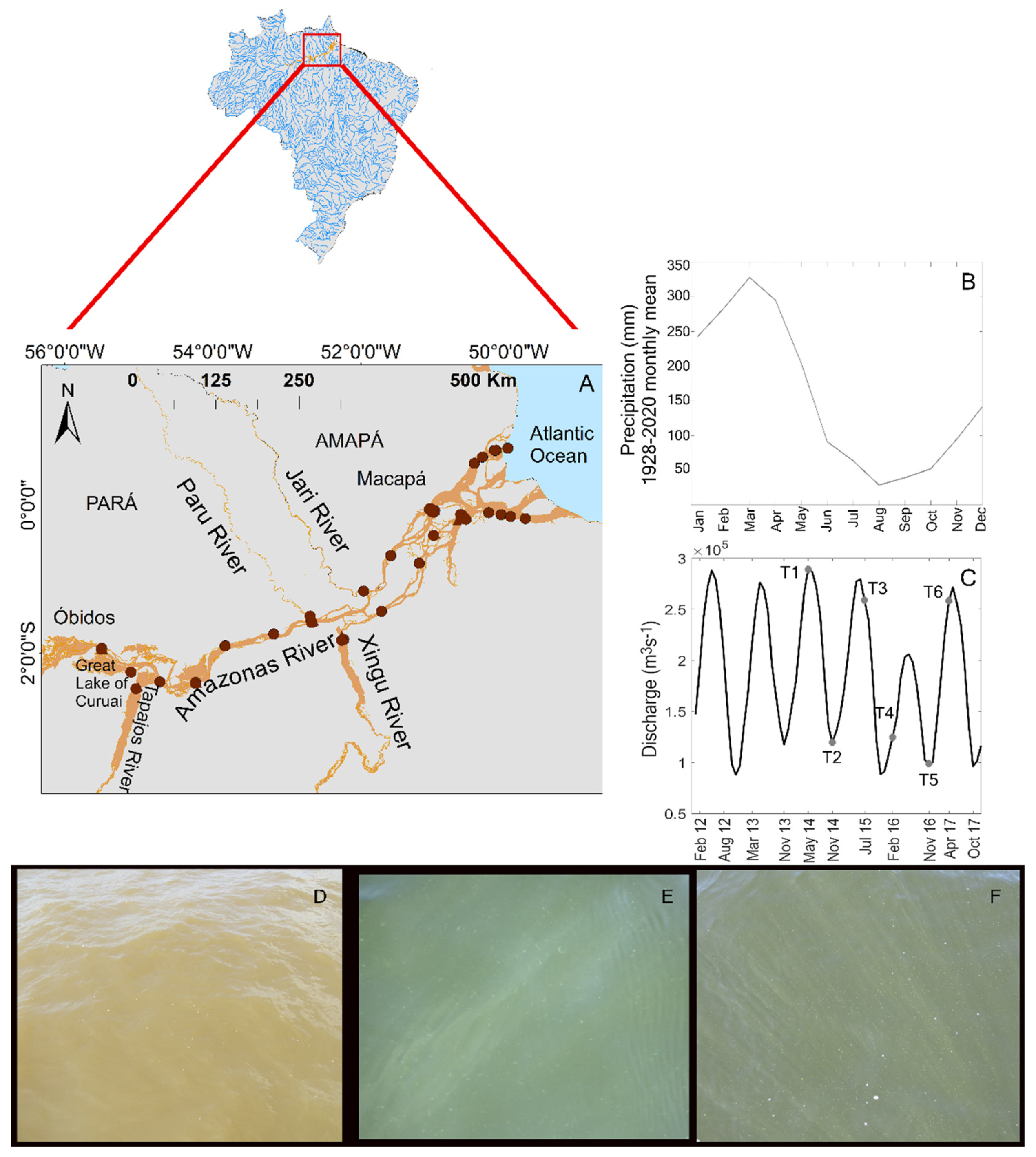
2.1. Study Area

The Lower Amazon study region comprises the area along a 900 km transect between the upstream boundary at Óbidos (01°55.141′ S, 55°31.543′ W) and the Amazon River mouth near the city of Macapá (Figure 1A). The wet season in the study area starts in November, with the peak in March (Figure 1B). The rising water discharge season starts at the end of December and reaches the high-water level peak in May. In June, the water level starts to fall, and the minimum is observed in November [32,33]. According to previous studies in this region [34,35], the seasonal discharge months are defined as (Figure 1C): rising water (January–March); high water (April–June); falling water (July–September); and low water (October–December).

Samples were collected at stations along the Amazon mainstem, in a series of expeditions by the research vessel M/V Mirage, at Óbidos, below Santarem, Almeirim, and two primary channels near the geographical river mouth by Macapá. At Óbidos, the width of the Amazon River is 2.3 km, and, at Macapá, each channel has a width of 11 km. The width of the mainstream at the Lower Amazon is stable and has little variation along the seasonal discharge [36].

The location of Óbidos is crucial for monitoring the dynamics of the Amazon basin. It is the furthest downstream monitoring gauge of the Brazilian National Water Agency (ANA) where the mainstem has already received the contribution from large rivers, such as the Solimões, Negro, and Madeira, and from other smaller tributaries. Downstream of Óbidos, the Amazon River receives the inputs from two large tributaries: the Tapajós and Xingu rivers. The downstream boundary of our study was the north and south channels near Macapá, which are the last two well-constrained channels near the Amazon River mouth (00°05.400′ S, 51°03.200′ W and 00°09.415′ S, 50°37.353′ W, respectively). In addition to the mainstem, samples were collected in Tapajós, Xingu, Paru, Jari, and Jaraçu rivers, as well as at the Great Lake of Curuai floodplain (Figure 1A). These rivers are classified as clearwater rivers (Figure 1E,F), according to Sioli [18], generally presenting high rates of primary production when compared with turbid Amazon River waters (Figure 1D) [35]. Sampling of Tapajós and Xingu rivers was performed upstream of their confluence with the Amazon River at a “lake-like” portion of these rivers, where the river becomes similar to a lentic system. The sampling at clearwater (CW) rivers was always performed near the outfall portion of the river and, therefore, under the Amazon River influence. The magnitude of the Amazon River influence over CW rivers varies with the river size and its proximity to the Amazon River mouth where semi-diurnal flow reversals are observed [37,38]. The seasonality of river discharge also moderates the influence of the mainstem upon the tributaries.

The dataset used in this study consists of in situ measurements of optically significant constituents and inherent optical properties acquired from 2014–2017 during different discharge seasons. The sampling period of 2014–2017 was marked by exceptional climate events. The year of 2014 was characterized by a record flood in the Amazon Basin that started with a La Niña event in 2012 increasing the rainfall regime and was followed by a positive sea surface temperature anomaly in the Tropical Atlantic south of the equator, and in the Western Tropical Pacific [39,40,41,42]. During the rising water season of 2014, the rainfall within the south-western Amazon basin was 80–100% above usual records [41], with a consequently higher river discharge (Figure 1C).

Conversely, the year of 2015–2016 was marked by a severe drought caused by an El Niño period (Figure 1C), especially in the eastern Amazon basin [43]. The anomalously low water levels may have caused a disconnection of the Amazon River from some streams and floodplains potentially resulting in lower inputs of organic matter to the river’s mainstem. The disconnection of floodplains and streams from the mainstem caused by the river’s receded water level typical of drought periods has also been noted by other authors [40].

2.2. In Situ Data

2.2.1. Above Water Radiometry

Above water radiometry was measured with a portable hyperspectral spectroradiometer FieldSpec® (ASD Inc., Boulder, CO, USA) which collects radiance (L, µW m⁻² sr⁻¹) in the range of 350 to 1100 nm (bandwidth 1 nm) and a field-of-view of 25°. The acquisition geometry followed Mobley [44] recommendations to avoid shadows and sunglint contamination in the measurements. The radiance measurements were conducted between 09:00 a.m. to 04:00 p.m. local time. Total water leaving radiance (L_w), sky radiance (L_sky), and the radiance from a white panel Spectralon reference (L_g) were consecutively measured 10 times. The latter parameter was used to estimate the downwelling irradiance (E_d) (Equation (1)):

$$E_d\left(\lambda \right)=L_g\left(\lambda \right)f_c\pi ,$$

(1)

where f_c is a correction factor estimated in laboratory by the ratio of a standard Spectralon reference that remains in the laboratory by the Spectralon panel used during fieldwork.

The remote sensing reflectance (R_rs) is computed according to Equation (2):

$$R_{rs}=\frac{L_w}{E_d}=\frac{L_u-{\rho }_{air-river}\ast L_{sky}}{E_d },$$

(2)

where L_u is the upwelling radiance that reaches the sensor, and ${\rho }_{air-river}$ is a sky glint correction coefficient at the air-sea interface.

There are several methods in the literature to correct the optical signal from sunglint interference. In the present study, we used the approach of Ruddick et al. [45], which is indicated for turbid to highly turbid waters. The ${\rho }_{air-river}$ is a function of wind and cloud cover (Equations (3) and (4)).

$$\frac{L_{sky}\left(\lambda =750\right)}{E_D\left(\lambda =750\right)}\ge 0.05 \to {\rho }_{air-river}=0.0256,$$

(3)

or

$$\frac{L_{sky}\left(\lambda =750\right)}{E_D\left(\lambda =750\right)}<0.05 \to {\rho }_{air-river}=0.0256+0.00039W+0.000034W^2,$$

(4)

where W is the wind measured concurrently with the radiometric measurements.

The residual glint or white offset correction was not performed for the spectra dataset. According to Ruddick et al. [46], this correction is usually based on NIR spectrum (e.g., $R_{rs}\left(780\right)$ and $R_{rs}\left(720\right))$ assuming that its shape is largely determined by pure water absorption. In very turbid waters, like in the Amazon River, the NIR assumption is not verified, and the NIR spectrum still has a high water signal.

2.2.2. Bio-Optical Measurements

Surface water samples for bio-optical measurements were acquired at all stations and filtered aboard the ship up to one hour after collection under gentle vacuum (<5 mm Hg), according to Mitchell et al.’s [47] protocol. Sub-samples were later processed in the laboratory for the determination of light absorption coefficients by total particulate matter (a_p(λ) m⁻¹) and CDOM (a_CDOM(λ) m⁻¹) using a dual-beam Shimadzu UV-2450 spectrophotometer, equipped with an integration sphere, within the interval of 250–850 nm. Aliquots of surface water samples were also used for the determination of chla and SPM concentration. The filters for a_p and chla were stored in a portable ultrafreezer during the cruise and stored in liquid nitrogen until posterior analysis in the laboratory using a spectrophotometer and a fluorimeter, respectively.

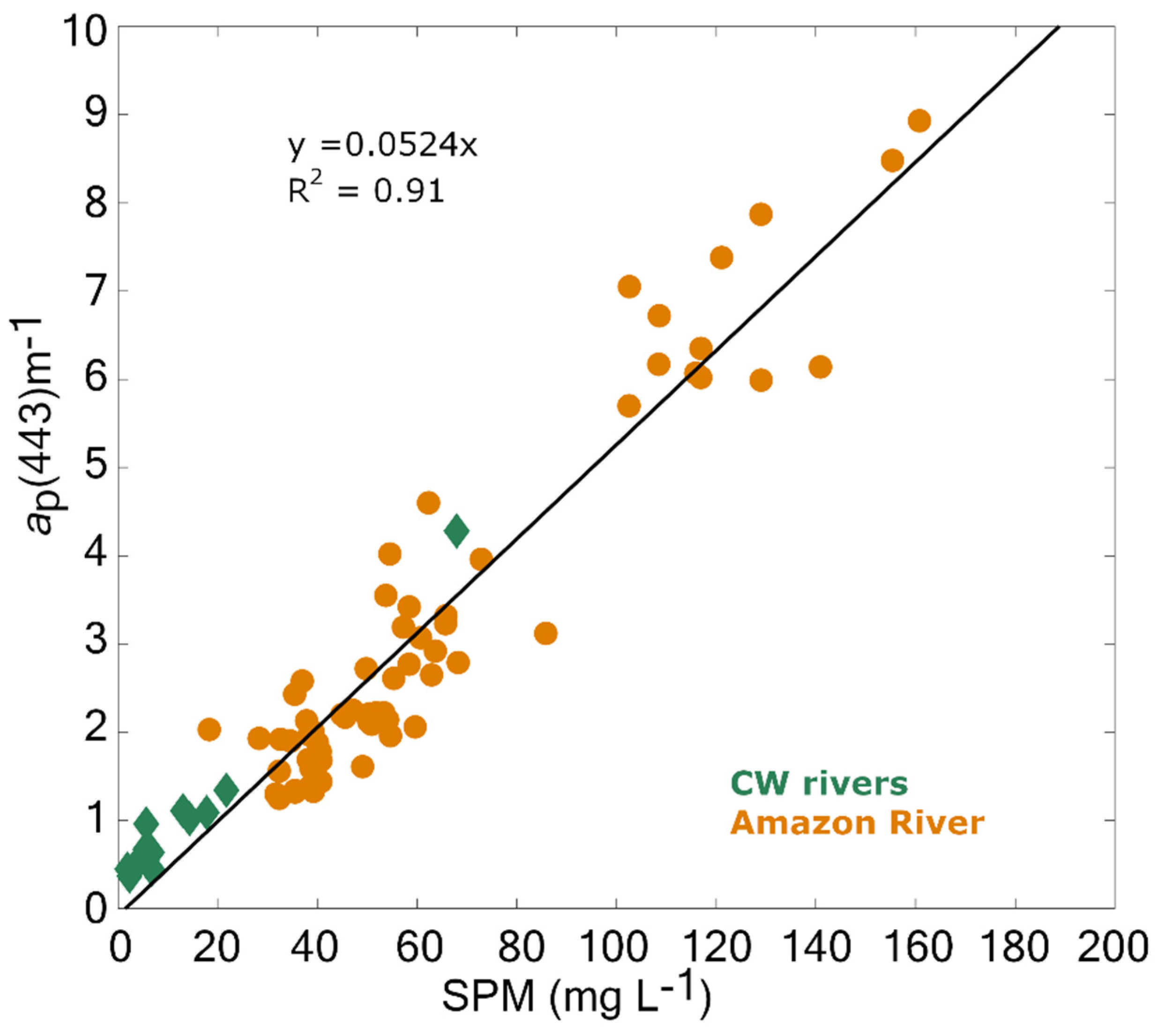
Light Absorption by Particulate Matter

Duplicate surface water samples were filtered through 25 mm Whatman GF/F glass fiber filters (0.7 µm nominal pore size). Water filtration was performed in order to obtain enough coloration of the filter pad, varying the volume between 10–125 mL depending on the river turbidity. The a_p spectra were calculated using the transmittance-reflectance (T-R) method [48]. The T-R method is preferentially recommended for particle-rich waters with the correction of the light backscattering by the particle sample with an integrating sphere. The slope of the absorption due to non-algal particles (a_nap(λ)), S_nap, computed over the 400–800 nm spectral domain (S_nap400–800) [49,50], potentially indicates the relative contribution of mineral and organic particles in the water [11]. In this study, we considered a_p as representative of NAP because a_phy contribution was very low for the Amazon and relatively low for CW rivers (<2% and <20% of a_p (443), respectively) that was under Amazon River influence.

Light Absorption by Colored Dissolved Organic Matter

After removing the larger suspended particles used to estimate a_p, the remaining filtered surface water samples were filtered again using 0.2 µm polycarbonate membranes (Whatman Nuclepore, 25 mm). Samples were stored in pre-combusted glass bottles (450 °C, 6 h) wrapped with aluminum foil and kept under refrigeration (4 °C) until further laboratory analysis. CDOM samples were exposed to room temperature before spectrophotometric analysis in order to avoid any bias due to the thermal difference between the samples and the reference Milli-Q water. a_CDOM(λ) was calculated from absorbance measurements as follows (Equation (5)):

$$a_{\mathrm{CDOM}}\left(\lambda \right)=2.303\frac{A\left(\lambda \right)}{L},$$

(5)

where A(λ) is the absorbance of the filtered water sample at the specific wavelength λ, and L is the optical pathway of the quartz cell in meters (here, 0.1 m).

As recommended by Babin et al. [11], a baseline correction was applied to each spectrum by subtracting the mean absorbance in the range of 680–690 nm from the whole spectrum. The absorption spectral shape of CDOM is estimated using a linear least-squares regression of the logarithm of a_CDOM(λ) and reported in units of nm⁻¹ [51] (Equation (6)):

$$a_{\mathrm{CDOM}}\left(\lambda \right)=a_{\mathrm{CDOM}}\left({\lambda }_0\right)e^{-S\left(\lambda -{\lambda }_0\right)},$$

(6)

where a_CDOM(λ) is the absorption coefficient at wavelength λ, a_CDOM(λ₀) is the absorption coefficient at a reference wavelength λ₀, and S is the spectral slope in the spectral range from λ₀ to λ, with λ₀ < λ.

Many studies have demonstrated the importance of the slope in the range of 275–295 nm (S_275–295) to assess the dissolved organic molecular weight [16,17,52,53]; therefore, this interval was adopted in this study.

The proportion of CDOM to the total absorption (a_CDOM: (a_CDOM + a_p)), and of particles to the total absorption (a_p: (a_CDOM + a_p)), except pure water, were also calculated at 443 nm.

Chlorophyll-a Concentration

The concentration of chla (µg L⁻¹) was measured from 25 to 100 mL of water samples filtered using 25 mm Whatman GF/F glass fiber filters (0.7 µm nominal pore size). At the laboratory, triplicate samples of pigments were extracted from the filters after immersion in 10 mL of 90% acetone/Dimethyl sulfoxide (DMSO) solution (60/40 by volume, according to Shoaf and Lium [54]) for 24 h, in the dark, at −10 °C. The resulting extraction was analyzed using a calibrated bench Turner Designs 10-AU fluorimeter.

Suspended Particulate Matter Concentration

Suspended particulate matter concentration (SPM, mg L⁻¹) was determined gravimetrically following the method of Van der Linde [55]. Before field work, 0.45 µm (nominal pore size) cellulose acetate filters (Millipore) were dried for 24 h, weighed (W₁), and placed in Petri plates for transportation. In the field, a volume (V) of 150 to 400 mL of surface water was filtered, and the filters for SPM were stored for further laboratory analysis. At the laboratory, SPM filters were dried for 72 h at 50 °C and weighed (W₂) to determine SPM according to Equation (7):

$$\frac{W_1-W_2}{V}\frac{W_1-W_2}{V}.$$

(7)

The number of samples collected in the Amazon and CW rivers are shown in

Table 1. Total number of in situ data gathered during the years of 2014–2017 in the Lower Amazon region.

Parameter	Amazon River	CW Rivers	Total Samples
aCDOM(λ) (m−1)	116	14	130
SCDOM(λ) (nm−1)	116	14	130
ap(λ) (m−1)	95	14	109
Sp(λ) (nm−1)	95	14	109
SPM (mg L−1)	90	12	102
chla (µg L−1)	85	12	97

.

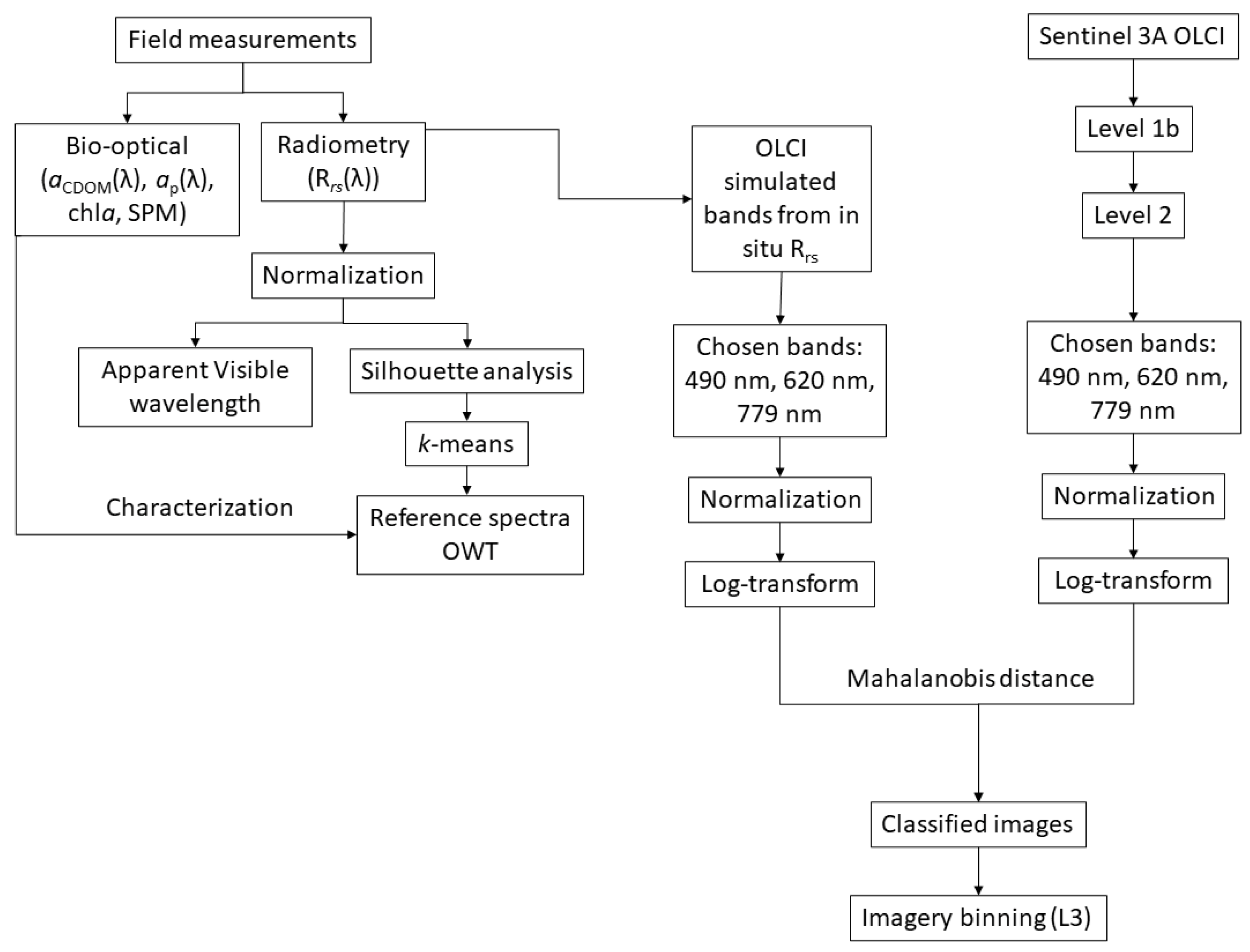
2.3. In Situ Rrs Classification

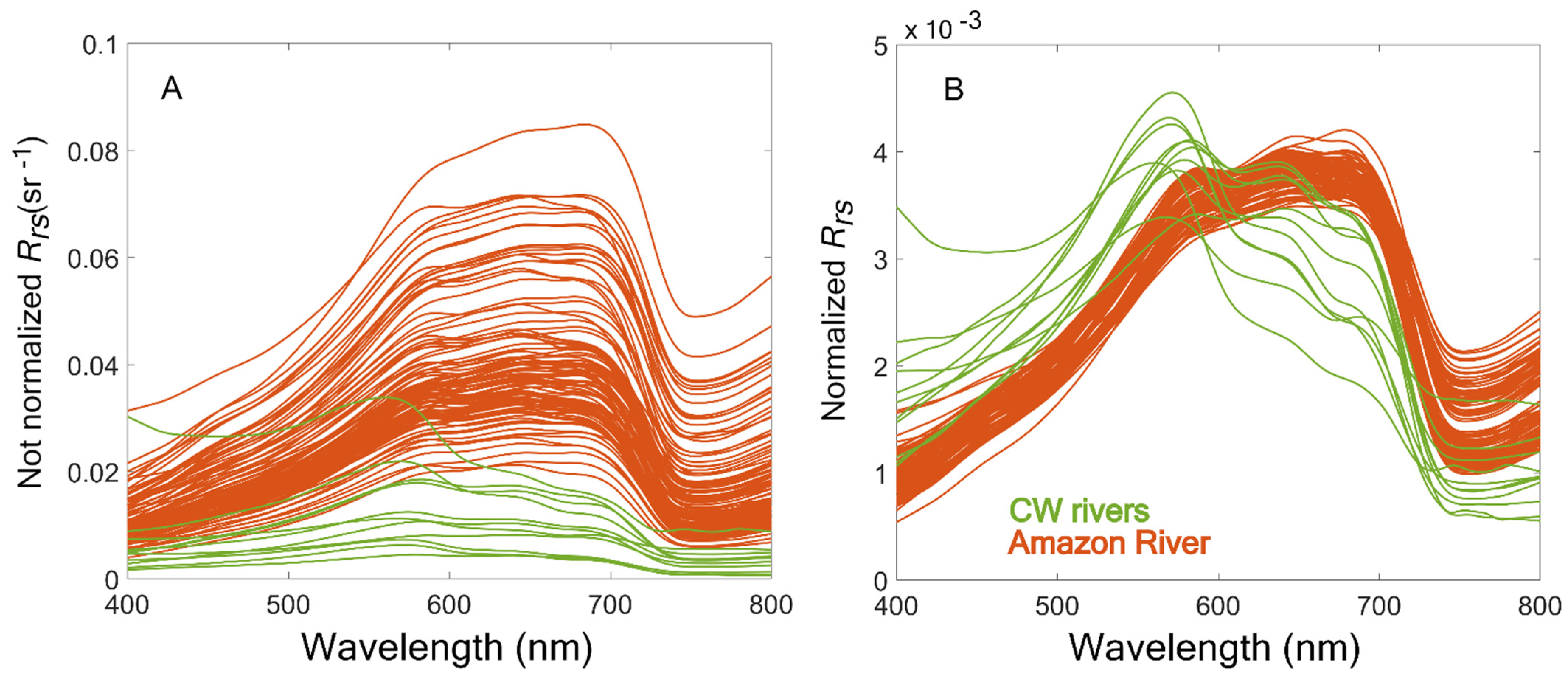
2.3.1. Spectra Normalization

Each R_rs spectrum was normalized by its integrated value [22,23,56] according to the Equation (8). The integration was computed using the trapezoidal method, over the 400–800 nm range.

$$r_n\left(\lambda \right)=\frac{R_{rs}\left(\lambda \right)}{{{\displaystyle \int }}_{{\lambda }_1}^{{\lambda }_2}{R}_{rs}\left(\lambda \right)d\lambda },$$

(8)

where $r_n\left(\lambda \right)$ (in units of nm⁻¹) is the normalized spectrum obtained by integration between ${\lambda }_1$ (400 nm) and ${\lambda }_2$ (800 nm).

The goal of the normalization is to reduce the first order variability of reflectance and focus on the reflectance spectral shape, hence removing amplitude differences caused by concentration variation. The normalization is a common step that precedes the optical classification procedure, as performed in previous studies [20,22,56,57]. Vantrepotte et al. [22] highlighted the importance of using normalized reflectance spectra instead of raw R_rs to perform an optical water type classification. For example, if a water body has a high concentration of SPM (e.g., the Amazon River), the use of raw R_rs would lead to a classification primarily based on the relative concentration of sediments, and, consequently, all other optically significant constituents contributions could be neglected.

2.3.2. Optical Water Type Identification

Different supervised and unsupervised methods have been used for the classification of R_rs with the aim of defining OWTs based upon differences in the magnitude and shape of the spectral curves [20,21,22,23,31,56,57,58]. Unsupervised classification can be used when a priori knowledge is not available, and R_rs data is used to define the clusters, thereby being less subject to user errors [59]. The k-means and fuzzy c-means are known techniques among the unsupervised classification methods [12,13,20,21,22,24,31,57]. When comparing k-means versus fuzzy c-means and other unsupervised methods (e.g., Ward algorithm), the clustering results can be very similar [20,22,59]. Therefore, k-means was adopted in this study to cluster the data into homogeneous optical groups.

k-means technique (Equation (9)) requires a user-specified number of clusters (k), which are represented by their centroids [60]. The clusters are defined by measuring the square Euclidian distance of the centroids. For this, an initial mean spectra (“seed”) is arbitrarily specified for each of the k-clusters. Then, each spectra of the dataset are assigned to the class whose mean spectra value is closest to the seed, forming the first set of decision boundaries. A new set of cluster seed is then calculated from this classification, and the spectra is reassigned accordingly, until there is no significant change in the spectra assignments from one iteration (i) to the next [59]. The Silhouette width analysis [61] was used to determine the number of clusters, by measuring how similar an individual point is to its own cluster.

$$\mathsf{\Delta }\mu \left(i\right)={{\displaystyle \sum }}_{k=1}^K|{\mu }_k^i-{\mu }_k^{i-1}|.$$

(9)

Another way to assess water color approached in this study was proposed by Vandermeulen et al. [62], by using the weighted harmonic mean of the R_rs(λ) that create an index called Apparent Visible Wavelength (AVW), in units of nanometers (Equation (10)):

$$AVW=\frac{{{\displaystyle \sum }}_{i={\lambda }_1}^{{\lambda }_n}{R}_{rs}\left({\lambda }_i\right)}{{{\displaystyle \sum }}_{i={\lambda }_1}^{{\lambda }_n}\frac{R_{rs}\left({\lambda }_i\right)}{{\lambda }_i}}={\left(\frac{{{\displaystyle \sum }}_{i={\lambda }_1}^{{\lambda }_n}{\lambda }_i{}^{-1}{R}_{rs}\left({\lambda }_i\right)}{{{\displaystyle \sum }}_{i={\lambda }_1}^{{\lambda }_n}{R}_{rs}\left({\lambda }_i\right)}\right)}^{-1}.$$

(10)

The dynamical spectral index proposed by Vandermeulen et al. [62] does not require a training dataset and/or defining the number of classes a priori. Instead, the result is given as a gradient of wavelengths values that represent a quantitative descriptor of weighted mean color reflected from the water surface. Both classification k-means and the AVW index were applied on the normalized R_rs(λ) spectra and, therefore, focus on the spectral shape. The AVW was used as a complement information, defining the thresholds of the determined classes.

2.4. Satellite Data

A set of 48 level 1 OLCI images from Sentinel-3 satellite (S3A) were downloaded from the Copernicus Online Data Access (https://coda.eumetsat.int/, accessed on 9 March 2021) and processed to level 2 and 3 using SeNtinel Applications Platform (SNAP) software, version 8.0.2. This imagery has a nominal spatial resolution of 300 m with a 14-bit radiometric resolution [26], and was processed to derive R_rs data. Initially, four images with low cloud coverage (<10%) and representative of each discharge season (rising water—3 January 2018, high water—27 June 2020, falling water—25 July 2017, low water—7 December 2017) were selected. From those four starting images, other ±10 days images were also downloaded and processed, with a total of 48 images. The level 2 images were derived using the Case 2 Regional Coast Color processor (C2RCC), and the flagged bright areas were removed from the scenes. The C2RCC is an atmospheric correction method that has an overall good performance over inland water [63].

The 490 nm, 620 nm, and 779 nm bands (B4, B7, and B16, respectively) were used for the classification approach. These bands were chosen by their potential for distinguishing classes, and, according to ESA [26], the band 620 nm is important to assess sediment loadings, while band 490 nm is relevant to assess chla [64]. The near infrared band at 779 nm is also relevant in waters with a high concentration of suspended sediments as in the study area [13].

2.4.1. Satellite R_rs(λ) Classification

The Mahalanobis distance was used to determine the separability of the given classes upon S3A images. The utilization of the Mahalanobis distance to distinguish the spectra among the classes has been applied in previous ocean color studies [22,56,65]. For this, OLCI bands were simulated utilizing in situ R_rs(λ) according to the spectral response function of the respective sensor bands. Later, the simulated B4, B7, and B16 bands were selected and normalized, as described in Equation 8. The normalized bands were then log-transformed. The same process was applied to OLCI B4, B7, and B16 bands, where the bands were normalized (Equation (8)) and log-transformed. The classification consisted of calculating statistically how much of a given unknown spectrum (x) belongs to a defined class according to the average spectrum, µ, and the covariance matrix, $\mathsf{\Sigma }$. The distance of the resulting input x to a given class ik was estimated by the squared Mahalanobis distance ${\mathsf{\Delta }}_{i{k}^2}$ (Equation (11)):

$${\mathsf{\Delta }}_{ik}^2\left(x\right)={\left(x-{\mu }_{ik}\right)}^T{{\displaystyle \sum }}_{ik}^{-1}(x-{\mu }_{ik})$$

(11)

where T indicates the matrix transpose. The probability (p) that an unknown spectrum (x) belongs to a class ik was estimated as (Equation (12)):

$$p\left(ik,x\right)=1-\frac{\gamma (n/2,{\mathsf{\Delta }}_{ik}^2\left(x\right)/2)}{\mathsf{\Gamma }\left(n/2\right)}$$

(12)

where $\mathsf{\Gamma }$is the gamma function, $\gamma$ is the lower incomplete gamma function, and $n$ is the number of the bands (3) used in the classification.

The normalized belonging $p^{*}$ was calculated as (Equation (13)):

$$p^{*}\left(ik\right)=\frac{p\left(ik\right)}{{{\displaystyle \sum }}_{ic=1}^{NC}p\left(ik\right)}$$

(13)

More details of how $p^{*}\left(ik\right)$and $p\left(ik,x\right)$ were calculated can be found in Vantrepotte et al. [22]. The algorithm developed to calculate the Mahalanobis distance, as well as $p^{*}\left(ik\right)$and $p\left(ik,x\right)$, was implemented in MATLAB programming language.

2.4.2. Satellite Pixels Labelling

The 48 classified OLCI images were temporally binned to represent the four discharge seasons. The $p^{*}\left(ik\right)$ of each image was averaged according to the respective season. The Mahalanobis classification was binned based on the mode, i.e., evaluating the maximum frequency of each class per pixel. The methodology used in this study is shown in Figure 2.

3. Results

3.1. General Bio-Optical Characterization of the Lower Amazon Region

Table 2. Bio-optical characteristics of clearwater rivers and Amazon River.

	Clearwater Rivers			Amazon River
	Average ± SD	CV %	Range	Average ± SD	CV %	Range
aCDOM(443) (m−1)	2.01 ± 0.88	44	0.74–3.53	2.12 ± 0.53	25	0.89–4.40
S275–295 (nm−1) × 10−2	1.47 ± 0. 14	10	1.32–1.85	1.45 ± 0. 05	3	1.30–1.66
ap(443) (m−1)	1.68 ± 2.44	145	0.37–9.44	3.16 ± 2.11	67	1.18–8.93
Sp400–800 (nm−1) × 10−2	1.05 ± 0. 13	12	0. 88–1.30	1.05 ± 0. 08	8	0. 91–1.33
SPM (mg L−1)	14.0 ± 18.1	129	1.8–67.9	69.7 ± 33.8	48	18.3–160.8
chla (µg L−1)	6.1 ± 7.7	126	1.5–31.3	1.4 ± 0.8	57	0.5–6.3
aCDOM:(aCDOM + ap)(443)	0.64 ± 0.19	30	0.17–0.80	0.44 ± 0.12	27	0.17–0.64
ap: (aCDOM + ap) (443)	0.36 ± 0.19	53	0.20–0.83	0.56 ± 0.12	21	0.36–0.83
ap(443): SPM	0.11 ± 0.05	45	0.06–0.24	0.05 ± 0.01	20	0.03–0.11

SD = Standard Deviation; CV = Coefficient of Variation.

summarizes the basic statistics of all samples obtained across the Lower Amazon region, disregarding the seasonality. Values of a_CDOM(443) of Amazon River and CW rivers are in a similar range, although the coefficient of variation of CW a_CDOM(443) (44%) are almost two-fold higher than the coefficient of variation of Amazon River a_CDOM(443) (25%). S_275–295 had a higher average value (0.0147 ± 0.0014 nm⁻¹) and a higher variability (10%) for CW river samples compared to Amazon River samples (3%).

The absorption coefficient of particulate matter (a_p(443)) is strongly correlated with SPM (R² = 0.91, p < 0.05, N = 77) (Figure 3), as previously reported by other studies in the Amazon basin [66]. The average ratio of a_p(443) : SPM is higher for CW rivers (CW: 0.11 ± 0.05; Amazon: 0.05 ± 0.01; see Table 2), with a 45% coefficient of variation (Amazon River CV: 20%). S_p showed similar values for Amazon and CW rivers (S_p400–800 $~$ 0.010 nm⁻¹), with low variability (Amazon 8% and CW rivers 12%) (see Table 2).

3.2. Seasonal Absorption Budget

Absorption by CDOM is dominant with a large contribution to the total absorption in CW rivers (a_CDOM(443) : a_CDOM(443) + a_p(443) = 0.64 ± 0.19 m⁻¹). However, its variability is similar (≅30%) to what is observed for the Amazon River (Table 2). In the Amazon River, although the absorption by particulate matter has a meaningful dominance, it is almost even with absorption by CDOM (a_CDOM 44%; a_p 56%; see Table 2). The balanced proportion among a_CDOM and a_p in the Amazon River is clearer when the absorption budget is assessed by hydrological season. Except for rising water, when a_p is almost three-fold higher than a_CDOM, all other seasons are nearly equivalent (

Table 3. Absorption budget of the Amazon River (Am) and clearwater rivers (CW) for rising water (RW), high water (HW), falling water (FW), and low water (LW) seasons.

		aCDOM: (aCDOM + ap) (443)		ap: (aCDOM + ap) (443)
		Average ± SD	CV %	Average ± SD	CV %
RW	Am	0.26 ± 0.08	31	0.74 ± 0.08	11
	CW	0.55 ± 0.26	47	0.45 ± 0.26	58
HW	Am	0.48 ± 0.09	19	0.52 ± 0.09	17
	CW	0.78 ± 0.03	4	0.22 ± 0.03	14
FW	Am	0.50 ± 0.07	14	0.50 ± 0.07	14
	CW	0.72 ± 0.06	8	0.28 ± 0.06	21
LW	Am	0.50 ± 0.05	10	0.50 ± 0.05	10
	CW	0.62 ± 0.06	10	0.38 ± 0.06	16

SD = Standard Deviation; CV = Coefficient of Variation.

). The variability is also greater during the rising water period for CW rivers, probably due to the influence of the overflow of the Amazon River that brings CDOM and SPM into the tributaries (Table 3).

3.3. Optical Classification

The advantage of using normalized spectra for clearly highlighting variation in water optical quality focusing on the shape of the R_rs spectra rather than on variation in R_rs amplitude (and thus on the turbidity level) is illustrated in Figure 4.

The Silhouette method indicated four as the optimal number of OWT classes to be used with the k-means clustering analysis of the in situ normalized R_rs between 400–800 nm (Figure 5A). Likewise, the AVW method presented the normalized R_rs as a gradient of wavelength values from which four central AVW could be detected (Figure 5B), according to the frequency distribution (histogram, not shown). For the k-means perspective, OWT k1 and k2 are representative of the Amazon River mainstem, OWT k3 is representative of the large CW tributaries (Tapajós and Xingu rivers), and k4 is representative of a mixture of other Amazonian water types, respectively. Herein, the OWT classes are named: k1 as Amazon Optical Water Type 1 (AOWT1), k2 as Amazon Optical Water Type 2 (AOWT2), k3 as Clear Optical Water Type (COWT), and k4 as Mixed Amazonian Optical Water Type (MAOWT) (Figure 4A).

The AOWT1 consisted in clustered in situ R_rs that were measured during the high, falling, and low water in the Amazon River (T1, T2, T3, and T5; see Figure 1C). The AVW of AOWT1 comprises the interval 584 nm ≤ AVW ≤ 598 nm, with the central wavelength at 590 nm (Figure 5B). Nevertheless, AOWT2 has an increasing reflectance in the same interval (green to NIR; see Figure 5) as a result of the immense input of sediments during the rising water season [66], with the central wavelength shifting to 605 nm in the range of 593 nm ≤ AVW ≤ 612 nm (Figure 5B). The AOWT2 class is primarily composed of water present during the period of rising water and high water seasons, corresponding to T4 and T6 field campaigns, respectively (Figure 1C).

The COWT class consists of R_rs spectra measured during the falling and low seasons in the large CW tributaries (Tapajós and Xingu rivers), in which the AVW comprises the interval 543 nm ≤ AVW ≤ 563 nm, with the central wavelength at 560 nm (Figure 5B).

The in situ R_rs spectra clustered in the MAOWT corresponds to rising water and high water periods in the CW rivers. MAOWT reflectance spectrum showed a less prominent chla peak in comparison to COWT, even though the average measured chla concentration was higher in comparison to other OWTs (

Table 4. Bio-optical characteristics of the four optical water types (OWT) identified for the Lower Amazon region.

	AOWT1		AOWT2		COWT		MAOWT
	59 Spectra		46 Spectra		4 Spectra		7 Spectra
	Average ± SD	Range	Average ± SD	Range	Average ± SD	Range	Average ± SD	Range
aCDOM	2.2 ± 0.6	1.3–4.2	2.0 ± 0.2	1.6–2.7	1.0 ± 0.3	0.7–1.3	2.4 ± 0.6	1.3–3.1
(443) (m−1)
S275–295 (nm−1) × 10−2	1.44 ± 0.05	1.32–1.54	1.45 ± 0.03	1.40–1.50	1.70 ± 0.17	1.51–1.85	1.41 ± 0.09	1.32–1.57
ap(443) (m−1)	2.03 ± 0.69	1.18–4.74	6.44 ± 1.61	2.72–9.44	0.48 ± 0.12	0.37–0.64	0.89 ± 0.25	0.50–1.11
Sp400–800 (nm−1) × 10−2	1.04 ± 0. 06	0.91–1.25	1.05 ± 0.07	0.95–1.26	0.93 ± 0.04	0.88–0.97	1.14 ± 0.14	0.95–1.30
SPM	43.6 ± 9.9	28.3–68.2	95.2 ± 29.4	49.8–157.2	4.4 ± 2.7	1.8–6.8	10.0 ± 5.8	3.7–17.8
(mg L−1)
chla	1.5 ± 0.8	0.5–4.4	1.4 ± 0.4	0.5–2.1	5.1 ± 2.9	2.3–8.5	9.1 ± 11.2	1.8–31.3
(mg L−1)
aCDOM: aCDOM + ap (443)	0.51 ± 0.06	0.28–0.64	0.25 ± 0.07	0.17–0.50	0.67 ± 0.10	0.55–0.78	0.73 ± 0.05	0.66–0.80
ap: aCDOM + ap (443)	0.49 ± 0.06	0.36–0.72	0.75 ± 0.07	0.50–0.83	0.33 ± 0.10	0.22–0.45	0.27 ± 0.05	0.20–0.34

). Another characteristic of MAOWT is a higher signal at the red-NIR spectrum when compared to COWT (Figure 5). The overflow of the Amazon River into CW rivers during the rising and high water seasons carries a large load of CDOM and SPM (Table 4). Therefore, the AVW of MAOWT is shifted to higher wavelengths in comparison to COWT, comprising the interval 569 nm ≤ AVW ≤ 581 nm, with the central wavelength at 575 nm (Figure 5B).

4. Discussion

4.1. CDOM Absorption

The Amazon River’s a_CDOM(443) values (2.12 ± 0.53 m⁻¹; see Table 2) are in the same range of values presented by Martinez et al. [13] (a_CDOM(440) = 3.3 ± 1.0 m⁻¹), and relatively lower when compared to values presented by Jorge et al. [67] (a_CDOM(420) ≅ 3.25 ± 0.46 m⁻¹) for Amazon white waters. CW rivers showed a similar average a_CDOM(443) value (2.01 ± 0.88 m⁻¹; see Table 2) in comparison to values reported by Martinez et al. [13] (a_CDOM(440) = 1.8 ± 0.8 m⁻¹). The discrepancies between a_CDOM values from different studies can be attributed to differences in each dataset size and representativeness, alternative filtering methods, chosen wavelengths, and protocol measurements (no baseline correction in Martinez et al. [13], for instance), as well as to different sampling locations and seasonality (e.g., Jorge et al. [67] sampled only during the rising water season in the Amazonian lakes).

High S_275–295 values generally indicate lower molecular weight dissolved organic matter (DOM) [17]. This potentially suggests that photobleaching has a larger impact on DOM composition in the CW rivers, which also receive less organic matter input from the terrestrial biosphere. A higher contribution of autochthonous DOM from phytoplankton in the CW rivers might also explain the observed variation [17,68], although a recent study demonstrated that S_275–295 is only slightly sensitive to the impact of phytoplankton-derived DOM [69]. The greater presence of phytoplankton in the CW rivers can be evidenced by high values of chla in comparison to the Amazon River (average of 6.1 and 1.4 µg L⁻¹, respectively; see Table 2). The higher variability of S_275–295 (CV: 10% for CW and 3% for the Amazon River; see Table 2), and other parameters in the CW rivers might be related to the location where the samples were collected, very close to the Amazon River mainstem, where turbid Amazon River waters may inflow into the smaller tributaries depending on the discharge season.

4.2. Particulate Matter Absorption

The slope of the regression between a_p and SPM (0.053; see Figure 3) is much higher than what is reported for coastal waters ($~$0.031) [11,70], and for combusted particles (0.024) [71], possibly due to an abundance of organic particles. CW river a_p(443) values are related to low concentrations of SPM (Table 2). Amazon River samples with SPM > 100 mg L⁻¹ were mainly obtained during the rising water season, indicating that the CW rivers may have more organic particles and may be more influenced by the Amazon River mainstem seasonality.

The Amazon and CW rivers S_p presented relatively lower values than what is usually reported for coastal and oceanic waters (>0.011 nm⁻¹) [11,50,72,73,74]. Previous studies showed that S_nap values of about 0.011 nm⁻¹ are typical of mineral dominated waters [11,71,73,75], and higher S_nap (>0.011 nm⁻¹) are related to organic particles [11,75]. Nevertheless, recent studies found an opposite trend in CDOM-rich waters, where steeper S_nap are in fact associated with more inorganic suspended matter by DOM adsorption in mineral surfaces [14,15,49,70]. Considering the high values of CDOM in the study area, this situation may also apply in the Lower Amazon region, where the relatively lower values of S_p, in comparison to the literature dedicated to coastal and oceanic waters, are in fact related to organic particles.

4.3. Differences among the Optical Water Types of the Lower Amazon Region

The average spectral shape of the four resultant OWTs from the Lower Amazon are in general agreement with other studies in the Amazon Basin, with measurements upstream of Óbidos and at lakes and floodplains [13,67,76,77,78,79]. Besides the evident distinction between the Amazon and CW rivers, another prevailing difference is related to the seasonality of the in situ measured R_rs. In the Amazon River (AOWT1 and AOWT2), there is no clear chla signal, and, although the reflectance signal is dominated by SPM, it is possible to observe that AOWT1 has a uniform signal over a wide part of the spectrum from the green to near-infrared wavelengths (NIR).

As mentioned, the AOWT2 comprises in situ R_rs from rising water and high water (T4 and T6, respectively; see Figure 1C). The high water period in 2017 (T6) contrasts to 2014 (T1) because it approximately resembles a rising water season, as a consequence of the El Niño impact on river discharge in the previous year [43]. Before 2014, the discharge peak did not fluctuate as much as that observed for 2016 (Figure 1C). The rainfall normalization in 2016 flushed sediments and organic matter to the Amazon River that were stored in the floodplains and tributaries from the previous year. The impact of the 2015–2016 El Niño on bio-optical properties of the Lower Amazon region was also discussed by Valerio et al. [1]. It is worth noting that AOWT2 is the spectrum resulting from the impact of rain and increased discharge after a long drought period. This situation could be related to seasonality, as well as to exceptional climate events, during the study period.

The well-defined 560 nm peak of the COWT (Figure 5A) is related to the backscattering of phytoplankton cells [80], indicating chla contribution, as can be evidenced in Table 4. Although MAOWT has a higher chla in comparison to COWT (Table 4), its 560 nm peak is less evident. As can be evidenced in Table 4, MAOWT also has higher values of CDOM. When in abundance, CDOM can have a role in the light absorption of the shorter wavelengths of the visible spectrum [81], reducing the reflectance attributed to chla, while SPM (Table 4) also causes a higher signal in the red-NIR wavelengths.

The standard deviation of the MAOWT chla (9.1 ± 11.2 mg L⁻¹; see Table 4) indicates a large variability. Previous studies also documented a large variability of chla and phytoplankton blooms during the rising and high water season within CW rivers (e.g., Tapajós River) [82,83]. The optimal balance between the input of nutrients from the surrounding watershed and light availability is likely the cause of this variation. The water clarity of these rivers allows sunlight to penetrate deep into the water column, promoting high rates of primary production.

4.4. Seasonal Distribution of OWT at the Lower Amazon Region

OWT varied by season. During the rising water season (Figure 6A), the Amazon River mainstem was mostly classified as AOWT2, while the larger CW rivers (Tapajós and Xingu), other smaller rivers, lakes, and floodplains were mostly classified as MAOWT. The classes AOWT1 and COWT were almost inexistent, with some small patches in floodplains (AOWT1) and at the Tapajós and Xingu rivers (COWT).

Bio-optical properties of AOWT2 indicate a considerable increase in SPM (95.2 ± 29.4 mg L⁻¹), a_p(443) (6.44 ± 1.61 m⁻¹), and in the relative contribution of a_p to total absorption (75 %) in comparison with AOWT1 (Table 4). The impact of seasonality on the variability of radiometric and bio-optical properties of the Amazon basin was previously discussed by other studies in the region, especially during the rising water season when the Amazon River reaches its highest SPM concentrations [66,84,85,86]. This variability can impact the definition of regional bio-optical inversion models. For example, Valerio et al. [1] showed that the dissolved organic carbon (DOC) could not be retrieved using a single relationship between a_CDOM(412) and DOC. During the rising water season and other river discharge peak situation (i.e., caused by exceptional climate events), there is a decoupling of the relationship of CDOM-DOC. Hence, future efforts for retrieving DOC using an OWT classification approach at the Lower Amazon region require considering AOWT2 specifically.

During the high water season, the Amazon River mainstem is predominantly occupied by AOWT1 (Figure 6B). The relative contribution of a_p to total absorption is now lower than presented by AOWT2 (AOWT1 49%; AOWT2 75%; see Table 4), due to the decrease in SPM input (43.6 ± 9.9; see Table 4). Conversely, the relative contribution of a_CDOM to total absorption increased (AOWT1 51%; AOWT2 25%; see Table 4). The COWT is observed in the classified OLCI composite for the high water season as the dominant class in Tapajós and part of the Xingu River, with the lower SPM concentration in comparison to other classes (4.4 ± 2.7 mg L⁻¹; see Table 4). The probability of pixel belonging to a MAOWT in lakes, floodplains, smaller rivers, and CW river margins is high.

During the falling water season, the probability of a pixel being classified as COWT increased for CW rivers, especially the Xingu River (Figure 6C). The phytoplankton primary production rates could increase due to the receding of the Amazon River pulse, leading to an enrichment of dissolved nutrients and decrease in turbidity [87]. In the Amazon River mainstem, AOWT1 is still dominant, while MAOWT is dominant in lakes, floodplains, smaller rivers, and CW river margins.

During the low water season, the transient status of the Amazon River is evidenced (Figure 6D). For 07/12/2017 (±10 days), it is possible to observe a decrease in AOWT1 presence at the upstream region, while AOWT1 is still dominant downstream. By December, the discharge in the Lower Amazon region increases at Óbidos (Figure 6D), carrying SPM from the Andes [88]. This volume of water loaded with SPM pushes AOWT1 towards the Amazon River mouth. Lakes and floodplains of the Amazon River upstream are dominated by AOWT2, and COWT start to shrink as evidenced in the Xingu River. Conversely, MAOWT presented dominance in the Xingu, likely due to the overflow of the Amazon River and the input of SPM.

During all hydrologic seasons, AOWT2 was dominant at the Amazon River mouth (Figure 6), indicating high SPM concentrations, and high relative contribution of a_p to total absorption (Table 4), probably caused by the tidal influence on the lower reaches of the Amazon River. Near the Amazon River mouth, the tide can completely reverse the flow toward the river upstream, increasing the water residence time, turbulence [34], and consequently, sediment resuspension in the water column.

5. Conclusions

The present study describes the bio-optical and radiometric variability along the Lower Amazon region, considering different discharge seasons. The Amazon River and CW rivers a_CDOM showed similar values (in average), in agreement with previous studies in the region. CW rivers a_CDOM and S_275–295 presented a relatively higher variability, indicating the influence of the Amazon River overflow into the tributaries. Dissolved organic matter in the CW rivers had lower molecular weight compared to the Amazon River, as indicated by higher S_275–295 values. This indicates a higher impact of photobleaching rates in CW rivers and less organic matter input from the terrestrial biosphere.

The absorption coefficient of total particulate matter had a good relationship with SPM concentration, showing the presence of high concentration of organic particles, especially in CW rivers. As expected, CW rivers had the lowest values of SPM, while the Amazon River had the higher values, especially during rising water. The variability of a_p(443): SPM at CW rivers is also higher, indicating the influence of the Amazon River mainstem into the tributaries. Further studies are required to better understand the observed variability of S_p in the Lower Amazon region. At this point, it is not clear if the slope approach was able to trace the relative proportion of organic and inorganic particles, while this potential has already been underlined for marine coastal waters [11].

The k-means clustering analysis identified four distinct OWT, and the analysis was complemented using the optical index AVW that presented the threshold of the optical classes. Our results showed that the OWT in the Lower Amazon region are strongly seasonally dependent and impacted by exceptional climate events. Briefly, AOWT1 dominance occurs during the high water and falling water season, in the Amazon River mainstem. During the end of the low water season, river discharge starts to rise, surging water is carried with SPM from the Andes, and AOWT2 start to dominate the upstream region, pushing AOWT1 towards the Amazon River mouth. During the rising water season, AOWT2 dominates the Amazon River mainstem. In the largest CW rivers (Tapajós and Xingu), COWT dominance starts to increase during the high water season, with the peak in the falling water season, later decreasing during the low water season. MAOWT is dominant and/or codominant in almost all of the Lower Amazon region, with a higher contribution in smaller tributaries and lakes.

For the Amazon River, not only seasonality is important but also extreme climate events, such as the record flood of 2014 and the severe drought of 2015–2016, that occurred during the study period. AOWT1 class was defined with the clustering of in situ measured R_rs from falling water, low water, and high water from 2014 (T1), being representative of the general condition of the Amazon River spectrum, except for the rising water season. AOWT2 class was defined with the R_rs spectra from rising water and high water from 2017 (T6). The discrepancies between high water of 2014 and 2017 may be associated with the impact of the El Niño 2015–2016 on the Amazon River discharge. Hence, AOWT2 can also be related to the direct impact of rising discharge due to rainfall on the river optical signature after a long drought. The spectra rise from green to NIR can be associated with the considerable increase in SPM input.

This study corroborates that rising water season presents a specific optical signature when compared to the other hydrological seasons, being a hallmark for the Lower Amazon region. Although rising waters occur during the first trimester of the year, river discharge is impacted by climate events and, as a result, can make it difficult to delineate the seasonality. Therefore, the k-means classification, as well the optical index AVW proposed here, can be used to monitor the nature of the water masses of the Lower Amazon region, considering the influence of unusual events. Among those, we can cite distinctive hydrological seasonal patterns associated with climate events, or other anomalous conditions potentially caused by anthropogenic impacts. Our study showed that water type classes derived from k-means clustering analysis can be used to assess bio-optical properties of the Lower Amazon region. Similarly, the AVW optical index can also be used for this purpose, especially if a proper central wavelength in the AVW range is considered in the spectra gradient. The classification presented here can provide a framework to the development of remote sensing inversion models adjusted to the complexity of the Lower Amazon River waters.

References

1. Valerio, A.D.M.; Kampel, M.; Vantrepotte, V.; Ward, N.D.; Sawakuchi, H.O.; Less, D.F.D.S.; Neu, V.; Cunha, A.; Richey, J. Using CDOM optical properties for estimating DOC concentrations and pCO2 in the Lower Amazon River. Opt. Express 2018, 26, A657–A677. [Google Scholar] [CrossRef] [PubMed] [Green Version]
2. Ward, N.D.; Bianchi, T.; Medeiros, P.M.; Seidel, M.; Richey, J.E.; Keil, R.G.; Sawakuchi, H.O. Where Carbon Goes When Water Flows: Carbon Cycling across the Aquatic Continuum. Front. Mar. Sci. 2017, 4. [Google Scholar] [CrossRef] [Green Version]
3. Xenopoulos, M.A.; Downing, J.A.; Kumar, M.D.; Menden-Deuer, S.; Voss, M. Headwaters to oceans: Ecological and biogeochemical contrasts across the aquatic continuum. Limnol. Oceanogr. 2017, 62, S3–S14. [Google Scholar] [CrossRef]
4. Tyler, A.; Hunter, P.D.; Spyrakos, E.; Groom, S.; Constantinescu, A.M.; Kitchen, J. Developments in Earth observation for the assessment and monitoring of inland, transitional, coastal and shelf-sea waters. Sci. Total Environ. 2016, 572, 1307–1321. [Google Scholar] [CrossRef] [PubMed] [Green Version]
5. Palmer, S.; Kutser, T.; Hunter, P.D. Remote sensing of inland waters: Challenges, progress and future directions. Remote. Sens. Environ. 2015, 157, 1–8. [Google Scholar] [CrossRef] [Green Version]
6. Gardner, J.R.; Yang, X.; Topp, S.N.; Ross, M.R.V.; Altenau, E.H.; Pavelsky, T.M. The Color of Rivers. Geophys. Res. Lett. 2021, 48. [Google Scholar] [CrossRef]
7. Preisendorfer, R.W. Hydrological Optics; US Department of Commerce, National Oceanic and Atmospheric Administration: Silver Spring, MA, USA, 1976; Volume 1.
8. Prieur, L.; Sathyendranath, S. An optical classification of coastal and oceanic waters based on the specific spectral absorption curves of phytoplankton pigments, dissolved organic matter, and other particulate materials. Limol. Oceanogr. 1981, 26, 671–689. [Google Scholar] [CrossRef]
9. Sathyendranath, S. Reports of the International Ocean-Colour Coordinating Group. IOCCG 2000, 3, 140. [Google Scholar]
10. Bricaud, A.; Babin, M.; Morel, A.; Claustre, H. Variability in the chlorophyll-specific absorption coefficients of natural phyto-plankton: Analysis and parameterization. J. Geophys. Res. 1995, 100, 13321. [Google Scholar] [CrossRef]
11. Babin, M.; Stramski, D.; Ferrari, G.M.; Claustre, H.; Bricaud, A.; Obolensky, G.; Hoepffner, N. Variations in the light absorption coefficients of phytoplankton, nonalgal particles, and dissolved organic matter in coastal waters around Europe. J. Geophys. Res. Space Phys. 2003, 108. [Google Scholar] [CrossRef]
12. Neil, C.; Spyrakos, E.; Hunter, P.; Tyler, A. A global approach for chlorophyll-a retrieval across optically complex inland waters based on optical water types. Remote Sens. Environ. 2019, 229, 159–178. [Google Scholar] [CrossRef]
13. Martinez, J.-M.; Espinoza-Villar, R.; Armijos, E.; Moreira, L.S. The optical properties of river and floodplain waters in the Amazon River Basin: Implications for satellite-based measurements of suspended particulate matter. J. Geophys. Res. Earth Surf. 2015, 120, 1274–1287. [Google Scholar] [CrossRef]
14. Binding, C.; Jerome, J.; Bukata, R.; Booty, W. Spectral absorption properties of dissolved and particulate matter in Lake Erie. Remote Sens. Environ. 2008, 112, 1702–1711. [Google Scholar] [CrossRef]
15. Riddick, C.A.L.; Hunter, P.D.; Tyler, A.N.; Martinez-Vicente, V.; Horváth, H.; Kovacs, A.W.; Vörös, L.; Preston, T.; Présing, M. Spatial variability of absorption coefficients over a biogeochemical gradient in a large and optically complex shallow lake. J. Geophys. Res. Ocean. 2015, 120, 7040–7066. [Google Scholar] [CrossRef] [Green Version]
16. Fichot, C.G.; Benner, R. The spectral slope coefficient of chromophoric dissolved organic matter (S275–295) as a tracer of terrigenous dissolved organic carbon in river-influenced ocean margins. Limnol. Oceanogr. 2012, 57, 1453–1466. [Google Scholar] [CrossRef] [Green Version]
17. Helms, J.; Stubbins, A.; Ritchie, J.D.; Minor, E.; Kieber, D.J.; Mopper, K. Absorption spectral slopes and slope ratios as indicators of molecular weight, source, and photobleaching of chromophoric dissolved organic matter. Limnol. Oceanogr. 2008, 53, 955–969. [Google Scholar] [CrossRef] [Green Version]
18. Sioli, H. The Amazon. In Limnology and Landscape Ecology of a Mighty Tropical River and Its Basin; Springer: Cham, Switzerland, 1984; Volume 56, ISBN 9789400965447. [Google Scholar]
19. Jerlov, N.G. Marine Optics; Elsevier: New York, NY, USA, 1976; Volume 14, ISBN 9780444414908. [Google Scholar]
20. Spyrakos, E.; O’Donnell, R.; Hunter, P.D.; Miller, C.; Scott, M.; Simis, S.G.H.; Neil, C.; Barbosa, C.C.F.; Binding, C.E.; Bradt, S.; et al. Optical types of inland and coastal waters. Limnol. Oceanogr. 2017, 63, 846–870. [Google Scholar] [CrossRef] [Green Version]
21. Moore, T.S.; Dowell, M.D.; Bradt, S.; Verdu, A.R. An optical water type framework for selecting and blending retrievals from bio-optical algorithms in lakes and coastal waters. Remote Sens. Environ. 2014, 143, 97–111. [Google Scholar] [CrossRef] [Green Version]
22. Vantrepotte, V.; Loisel, H.; Dessailly, D.; Mériaux, X. Optical classification of contrasted coastal waters. Remote Sens. Environ. 2012, 123, 306–323. [Google Scholar] [CrossRef]
23. Lubac, B.; Loisel, H. Variability and classification of remote sensing reflectance spectra in the eastern English Channel and southern North Sea. Remote Sens. Environ. 2007, 110, 45–58. [Google Scholar] [CrossRef]
24. Da Silva, E.F.F.; Novo, E.M.L.D.M.; Lobo, F.D.L.; Barbosa, C.C.F.; Noernberg, M.A.; Rotta, L.H.D.S.; Cairo, C.T.; Maciel, D.; Júnior, R.F. Optical water types found in Brazilian waters. Limnology 2020, 22, 57–68. [Google Scholar] [CrossRef]
25. Kosuth, P.; Callède, J.; Laraque, A.; Filizola, N.; Guyot, J.L.; Seyler, P.; Fritsch, J.M.; Guimarães, V. Sea-tide effects on flows in the lower reaches of the Amazon River. Hydrol. Process. 2009, 23, 3141–3150. [Google Scholar] [CrossRef]
26. European Space Agency—ESA. Sentinel-3 OLCI Technical Guide. Available online: https://sentinel.esa.int/web/sentinel/user-guides/sentinel-3-olci (accessed on 15 April 2021).
27. Tarpanelli, A.; Iodice, F.; Brocca, L.; Restano, M.; Benveniste, J. River Flow Monitoring by Sentinel-3 OLCI and MODIS: Comparison and Combination. Remote Sens. 2020, 12, 3867. [Google Scholar] [CrossRef]
28. Soomets, T.; Uudeberg, K.; Jakovels, D.; Brauns, A.; Zagars, M.; Kutser, T. Validation and Comparison of Water Quality Products in Baltic Lakes Using Sentinel-2 MSI and Sentinel-3 OLCI Data. Sensors 2020, 20, 742. [Google Scholar] [CrossRef] [Green Version]
29. Pahlevan, N.; Smith, B.; Schalles, J.; Binding, C.; Cao, Z.; Ma, R.; Alikas, K.; Kangro, K.; Gurlin, D.; Hà, N.; et al. Seamless retrievals of chlorophyll-a from Sentinel-2 (MSI) and Sentinel-3 (OLCI) in inland and coastal waters: A machine-learning approach. Remote Sens. Environ. 2020, 240, 111604. [Google Scholar] [CrossRef]
30. Bi, S.; Li, Y.; Wang, Q.; Lyu, H.; Liu, G.; Zheng, Z.; Du, C.; Mu, M.; Xu, J.; Lei, S.; et al. Inland Water Atmospheric Correction Based on Turbidity Classification Using OLCI and SLSTR Synergistic Observations. Remote Sens. 2018, 10, 1002. [Google Scholar] [CrossRef] [Green Version]
31. Eleveld, M.A.; Ruescas, A.B.; Hommersom, A.; Moore, T.S.; Peters, S.W.M.; Brockmann, C. An Optical Classification Tool for Global Lake Waters. Remote Sens. 2017, 9, 420. [Google Scholar] [CrossRef] [Green Version]
32. Mertes, L.A.K.; Magadzire, T.T. Large Rivers from Space. In Large Rivers: Geomorphology and Management; John Wiley & Sons: Hoboken, NJ, USA, 2008; pp. 535–552. ISBN 9780470849873. [Google Scholar]
33. Martinez, J.-M.; Bourgoin, L.M.; Kosuth, P.; Seyler, F.; Guyot, J.L. Analysis of multitemporal MODIS and landsat 7 images acquired over amazonian floodplains lakes for suspended sediment concentrations retrieval. Int. Geosci. Remote Sens. Symp. 2004, 3, 2122–2124. [Google Scholar] [CrossRef]
34. Sawakuchi, H.O.; Neu, V.; Ward, N.D.; Barros, M.D.L.C.; Valerio, A.M.; Gagne-Maynard, W.; Cunha, A.; Less, D.F.S.; Diniz, J.E.M.; Brito, D.; et al. Carbon Dioxide Emissions along the Lower Amazon River. Front. Mar. Sci. 2017, 4. [Google Scholar] [CrossRef] [Green Version]
35. Ward, N.D.; Krusche, A.; Sawakuchi, H.O.; Brito, D.; Cunha, A.; Moura, J.M.S.; da Silva, R.; Yager, P.; Keil, R.G.; Richey, J.E. The compositional evolution of dissolved and particulate organic matter along the lower Amazon River—Óbidos to the ocean. Mar. Chem. 2015, 177, 244–256. [Google Scholar] [CrossRef]
36. Birkett, C.M. Contribution of the TOPEX NASA Radar Altimeter to the global monitoring of large rivers and wetlands. Water Resour. Res. 1998, 34, 1223–1239. [Google Scholar] [CrossRef]
37. Ferraz, L.A.D.C. Tidal and Current Prediction for the Amazon’s North Channel Using a Hydrodynamical-Numerical Model. Ph.D. Thesis, Naval Postgraduate School, Monterey, CA, USA, 1975. [Google Scholar] [CrossRef] [Green Version]
38. Ward, N.D.; Sawakuchi, H.O.; Neu, V.; Less, D.; Valerio, A.M.; Cunha, A.C.; Kampel, M.; Bianchi, T.S.; Krusche, A.V.; Richey, J.E.; et al. Velocity-amplified microbial respiration rates in the lower Amazon River. Limnol. Oceanogr. Lett. 2018, 3, 265–274. [Google Scholar] [CrossRef]
39. Valerio, A.M.; Kampel, M.; Ward, N.D.; Sawakuchi, H.O.; Cunha, A.C.; Richey, J.E. CO2 partial pressure and fluxes in the Amazon River plume using in situ and remote sensing data. Cont. Shelf Res. 2021, 215, 104348. [Google Scholar] [CrossRef]
40. A Marengo, J.; Espinoza, J.C. Extreme seasonal droughts and floods in Amazonia: Causes, trends and impacts. Int. J. Clim. 2015, 36, 1033–1050. [Google Scholar] [CrossRef]
41. Espinoza, J.C.; Marengo, J.A.; Ronchail, J.; Carpio, J.M.; Flores, L.N.; Guyot, J.L. The extreme 2014 flood in south-western Amazon basin: The role of tropical-subtropical South Atlantic SST gradient. Environ. Res. Lett. 2014, 9, 124007. [Google Scholar] [CrossRef]
42. Satyamurty, P.; Da Costa, C.P.W.; Manzi, A.O.; Candido, L.A. A quick look at the 2012 record flood in the Amazon Basin. Geophys. Res. Lett. 2013, 40, 1396–1401. [Google Scholar] [CrossRef]
43. Jiménez-Muñoz, J.C.; Mattar, C.; Barichivich, J.; Santamaría-Artigas, A.S.; Takahashi, K.; Malhi, Y.; Sobrino, J.A.; Van Der Schrier, G. Record-breaking warming and extreme drought in the Amazon rainforest during the course of El Niño 2015–2016. Sci. Rep. 2016, 6, 33130. [Google Scholar] [CrossRef] [Green Version]
44. Mobley, C.D. Estimation of the remote-sensing reflectance from above-surface measurements. Appl. Opt. 1999, 38, 7442–7455. [Google Scholar] [CrossRef]
45. Ruddick, K.G.; De Cauwer, V.; Park, Y.-J.; Moore, G. Seaborne measurements of near infrared water-leaving reflectance: The similarity spectrum for turbid waters. Limnol. Oceanogr. 2006, 51, 1167–1179. [Google Scholar] [CrossRef] [Green Version]
46. Ruddick, K.; De Cauwer, V.; Mol, B. Van Use of the near infrared similarity reflectance spectrum for the quality control of remote sensing data. Remote Sens. Coast. Ocean. Environ. 2005, 588501. [Google Scholar]
47. Mitchell, B.G.; Kahru, M.; Wieland, J.; Stramska, M.; Mueller, J.L. Determination of spectral absorption coefficients of particles, dissolved material and phytoplankton for discrete water samples. Ocean Opt. Protoc. Satell. Ocean Color Sens. Valid. Revis. 2002, 3, 231. [Google Scholar]
48. Tassan, S.; Ferrari, G.M. A sensitivity analysis of the “Transmittance—Reflectance” method for measuring light absorption by aquatic particles. J. Plankt. Res. 2002, 24, 757–774. [Google Scholar] [CrossRef]
49. Estapa, M.L.; Boss, E.; Mayer, L.M.; Roesler, C.S. Role of iron and organic carbon in mass-specific light absorption by particulate matter from Louisiana coastal waters. Limnol. Oceanogr. 2011, 57, 97–112. [Google Scholar] [CrossRef] [Green Version]
50. Vantrepotte, V.; Brunet, C.; Mériaux, X.; Lécuyer, E.; Vellucci, V.; Santer, R. Bio-optical properties of coastal waters in the Eastern English Channel. Estuar. Coast. Shelf Sci. 2007, 72, 201–212. [Google Scholar] [CrossRef]
51. Bricaud, A.; Morel, A.; Prieur, L. Absorption by dissolved organic matter of the sea (yellow substance) in the UV and visible Domains. Limnol. Oceanogr. 1981, 26, 43–53. [Google Scholar] [CrossRef]
52. Vantrepotte, V.; Danhiez, F.-P.; Loisel, H.; Ouillon, S.; Mériaux, X.; Cauvin, A.; Dessailly, D. CDOM-DOC relationship in contrasted coastal waters: Implication for DOC retrieval from ocean color remote sensing observation. Opt. Express 2015, 23, 33–54. [Google Scholar] [CrossRef]
53. Fichot, C.G.; Benner, R. A novel method to estimate DOC concentrations from CDOM absorption coefficients in coastal waters. Geophys. Res. Lett. 2011, 38. [Google Scholar] [CrossRef]
54. Shoaf, W.T.; Lium, B.W. Improved extraction of chlorophyll a and b from algae using dimethyl sulfoxide. Limnol. Oceanogr. 1976, 21, 926–928. [Google Scholar] [CrossRef]
55. Van der Linde, D.W. Protocol for determination of total suspended matter in oceans and coastal zones. JRC Tech. Note I 1998, 98, 182. [Google Scholar]
56. Mélin, F.; Vantrepotte, V. How optically diverse is the coastal ocean? Remote Sens. Environ. 2015, 160, 235–251. [Google Scholar] [CrossRef]
57. Shen, Q.; Li, J.; Zhang, F.; Sun, X.; Li, J.; Li, W.; Zhang, B. Classification of Several Optically Complex Waters in China Using in Situ Remote Sensing Reflectance. Remote Sens. 2015, 7, 14731–14756. [Google Scholar] [CrossRef] [Green Version]
58. Shi, K.; Li, Y.; Zhang, Y.; Li, L.; Lv, H.; Song, K. Classification of Inland Waters Based on Bio-Optical Properties. IEEE J. Sel. Top. Appl. Earth Obs. Remote Sens. 2013, 7, 543–561. [Google Scholar] [CrossRef]
59. Schowengerdt, R.A. Techniques for Image Processing and Classifications in Remote Sensing; Academic Press: Cambridge, MA, USA, 2012. [Google Scholar]
60. Wilks, D.S. Statistical methods in the atmospheric sciences. In International Geophysics Series, 2nd ed.; Academic Press: Cambridge, MA, USA, 2006; ISBN 978-0-12-751966-1. [Google Scholar]
61. Rousseeuw, P.J. Silhouettes: A graphical aid to the interpretation and validation of cluster analysis. J. Comput. Appl. Math. 1987, 20, 53–65. [Google Scholar] [CrossRef] [Green Version]
62. Vandermeulen, R.A.; Mannino, A.; Craig, S.E.; Werdell, P.J. 150 shades of green: Using the full spectrum of remote sensing reflectance to elucidate color shifts in the ocean. Remote Sens. Environ. 2020, 247, 111900. [Google Scholar] [CrossRef]
63. Warren, M.; Simis, S.; Martinez-Vicente, V.; Poser, K.; Bresciani, M.; Alikas, K.; Spyrakos, E.; Giardino, C.; Ansper, A. Assessment of atmospheric correction algorithms for the Sentinel-2A MultiSpectral Imager over coastal and inland waters. Remote Sens. Environ. 2019, 225, 267–289. [Google Scholar] [CrossRef]
64. Werdell, P.J.; Bailey, S.W.; Franz, B.A.; Harding, L.W., Jr.; Feldman, G.C.; McClain, C.R. Regional and seasonal variability of chlorophyll-a in Chesapeake Bay as observed by SeaWiFS and MODIS-Aqua. Remote Sens. Environ. 2009, 113, 1319–1330. [Google Scholar] [CrossRef]
65. Mélin, F.; Vantrepotte, V.; Clerici, M.; D’Alimonte, D.; Zibordi, G.; Berthon, J.-F.; Canuti, E. Multi-sensor satellite time series of optical properties and chlorophyll-a concentration in the Adriatic Sea. Prog. Oceanogr. 2011, 91, 229–244. [Google Scholar] [CrossRef]
66. Pinet, S.; Martinez, J.-M.; Ouillon, S.; Lartiges, B.; Villar, R.E. Variability of apparent and inherent optical properties of sediment-laden waters in large river basins—lessons from in situ measurements and bio-optical modeling. Opt. Express 2017, 25, A283–A310. [Google Scholar] [CrossRef]
67. Jorge, D.S.F.; Barbosa, C.C.F.; De Carvalho, L.A.S.; Affonso, A.G.; Lobo, F.D.L.; Novo, E.M.L.D.M. SNR (Signal-To-Noise Ratio) Impact on Water Constituent Retrieval from Simulated Images of Optically Complex Amazon Lakes. Remote Sens. 2017, 9, 644. [Google Scholar] [CrossRef] [Green Version]
68. Gagne-Maynard, W.C.; Ward, N.D.; Keil, R.G.; Sawakuchi, H.O.; Cunha, A.; Neu, V.; Brito, D.; Less, D.F.D.S.; Diniz, J.E.M.; Valerio, A.D.M.; et al. Evaluation of Primary Production in the Lower Amazon River Based on a Dissolved Oxygen Stable Isotopic Mass Balance. Front. Mar. Sci. 2017, 4. [Google Scholar] [CrossRef] [Green Version]
69. Danhiez, F.P.; Vantrepotte, V.; Cauvin, A.; Lebourg, E.; Loisel, H. Optical properties of chromophoric dissolved organic matter during a phytoplankton bloom. Implication for DOC estimates from CDOM absorption. Limnol. Oceanogr. 2017, 62, 1409–1425. [Google Scholar] [CrossRef]
70. Xi, H.; Larouche, P.; Tang, S.; Michel, C. Seasonal variability of light absorption properties and water optical constituents in Hudson Bay, Canada. J. Geophys. Res. Ocean. 2013, 118, 3087–3102. [Google Scholar] [CrossRef]
71. Bowers, D.G.; Harker, G.E.L.; Stephan, B. Absorption spectra of inorganic particles in the Irish Sea and their relevance to remote sensing of chlorophyll. Int. J. Remote Sens. 1996, 17, 2449–2460. [Google Scholar] [CrossRef]
72. Zhang, X.; Huot, Y.; Bricaud, A.; Sosik, H.M. Inversion of spectral absorption coefficients to infer phytoplankton size classes, chlorophyll concentration, and detrital matter. Appl. Opt. 2015, 54, 5805–5816. [Google Scholar] [CrossRef]
73. Tzortziou, M.; Subramaniam, A.; Herman, J.; Gallegos, C.; Neale, P.J.; Harding, J.L.W. Remote sensing reflectance and inherent optical properties in the mid Chesapeake Bay. Estuar. Coast. Shelf Sci. 2007, 72, 16–32. [Google Scholar] [CrossRef]
74. Bricaud, A.; Morel, A.; Babin, M.; Allali, K.; Claustre, H. Variations of light absorption by suspended particles with chlorophyll a concentration in oceanic (case 1) waters: Analysis and implications for bio-optical models. J. Geophys. Res. 1998, 103, 31033–31044. [Google Scholar] [CrossRef]
75. Ferrari, G.M.; Bo, F.G.; Babin, M. Geo-chemical and optical characterizations of suspended matter in European coastal waters. Estuar. Coast. Shelf Sci. 2003, 57, 17–24. [Google Scholar] [CrossRef]
76. Yepez, S.; Laraque, A.; Martinez, J.-M.; De Sa, J.; Carrera, J.M.; Castellanos, B.; Gallay, M.; Lopez, J.L. Retrieval of suspended sediment concentrations using Landsat-8 OLI satellite images in the Orinoco River (Venezuela). Comptes Rendus Geosci. 2018, 350, 20–30. [Google Scholar] [CrossRef]
77. Martins, V.S.; Barbosa, C.C.F.; De Carvalho, L.A.S.; Jorge, D.S.F.; Lobo, F.D.L.; Novo, E.M.L.D.M. Assessment of Atmospheric Correction Methods for Sentinel-2 MSI Images Applied to Amazon Floodplain Lakes. Remote Sens. 2017, 9, 322. [Google Scholar] [CrossRef] [Green Version]
78. De Carvalho, L.A.S.; Barbosa, C.C.F.; Novo, E.M.L.D.M.; Rudorff, C.D.M. Implications of scatter corrections for absorption measurements on optical closure of Amazon floodplain lakes using the Spectral Absorption and Attenuation Meter (AC-S-WETLabs). Remote Sens. Environ. 2015, 157, 123–137. [Google Scholar] [CrossRef]
79. Lobo, F.D.L.; Novo, E.M.L.D.M.; Barbosa, C.C.F.; Galvão, L.S. Reference spectra to classify Amazon water types. Int. J. Remote Sens. 2011, 33, 3422–3442. [Google Scholar] [CrossRef]
80. Lain, L.R.; Bernard, S. The Fundamental Contribution of Phytoplankton Spectral Scattering to Ocean Colour: Implications for Satellite Detection of Phytoplankton Community Structure. Appl. Sci. 2018, 8, 2681. [Google Scholar] [CrossRef] [Green Version]
81. Joshi, I.; D’Sa, E.J. Seasonal Variation of Colored Dissolved Organic Matter in Barataria Bay, Louisiana, Using Combined Landsat and Field Data. Remote Sens. 2015, 7, 12478–12502. [Google Scholar] [CrossRef] [Green Version]
82. Albéric, P.; Pérez, M.A.; Moreira-Turcq, P.; Benedetti, M.F.; Bouillon, S.; Abril, G. Variation of the isotopic composition of dissolved organic carbon during the runoff cycle in the Amazon River and the floodplains. C. R. Geosci. 2018, 350, 65–75. [Google Scholar] [CrossRef]
83. Costa, M.P.F.; Novo, E.M.L.M.; Telmer, K.H. Spatial and temporal variability of light attenuation in large rivers of the Amazon. Hydrobiology 2012, 702, 171–190. [Google Scholar] [CrossRef]
84. Park, E.; Latrubesse, E. Surface water types and sediment distribution patterns at the confluence of mega rivers: The Solimões-Amazon and Negro Rivers junction. Water Resour. Res. 2015, 51, 6197–6213. [Google Scholar] [CrossRef]
85. Park, E.; Latrubesse, E.M. Modeling suspended sediment distribution patterns of the Amazon River using MODIS data. Remote Sens. Environ. 2014, 147, 232–242. [Google Scholar] [CrossRef]
86. Villar, R.E.; Martinez, J.-M.; Le Texier, M.; Guyot, J.L.; Fraizy, P.; Meneses, P.R.; de Oliveira, E. A study of sediment transport in the Madeira River, Brazil, using MODIS remote-sensing images. J. S. Am. Earth Sci. 2013, 44, 45–54. [Google Scholar] [CrossRef]
87. Novo, E.M.L.D.M.; Barbosa, C.C.F.; De Freitas, R.M.; Shimabukuro, Y.E.; Melack, J.M.; Filho, W.P. Seasonal changes in chlorophyll distributions in Amazon floodplain lakes derived from MODIS images. Limnology 2006, 7, 153–161. [Google Scholar] [CrossRef]
88. Filizola, N.; Guyot, J.L. Suspended sediment yields in the Amazon basin: An assessment using the Brazilian national data set. Hydrol. Process. 2009, 23, 3207–3215. [Google Scholar] [CrossRef]
Figure 1. (A) Sampling points along the Lower Amazon region during 2014–2017 field campaigns; (B) 1928–2020 monthly mean precipitation; (C) seasonal discharge of the Amazon River during 2012–2017 with field campaigns indicated (T1–T6). Discharge and precipitation data were acquired at the Óbidos station (National Water Agency of Brazil, ANA, www.ana.gov.br, (accessed on 9 March 2021)); (D) Amazon River water color, 16 July 2015; (E) Xingu River water color, 12 July 2015; (F) Tapajos River water color, 7 July 2015.
Remotesensing 13 03057 g001
Figure 2. Methodological framework showing all the steps used to develop this study.
Remotesensing 13 03057 g002
Figure 3. Scatterplot of ap(443) as a function of suspended particulate matter. A linear regression with null intercept is shown by the solid black line.
Remotesensing 13 03057 g003
Figure 4. (A) Not normalized in situ measured Rrs; (B) normalized in situ measured Rrs for the Lower Amazon region.
Remotesensing 13 03057 g004
Figure 5. (A) Average normalized Rrs spectra resultant from the k-means clustering analysis of the Lower Amazon region; (B) AVW values derived from the normalized in situ Rrs spectra (400–800 nm), yielding a range of values from 543 nm to 612 nm. The thicker lines with circle markers are referred to the central AVW according to the k-means classes.
Remotesensing 13 03057 g005
Figure 6. Inset, mean seasonal discharge of the Lower Amazon (2005–2015), with the seasonal sampling shown in red; Mahalanobis classification with the Amazon Optical Water Type 1 (AOWT1) in yellow, Amazon Optical Water Type 2 (AOWT2) in red, Clear Optical Water Type (COWT) in green, and Mixed Amazonian Water Type (MAOWT) in blue. (A) rising water image composite; (B) high water composite; (C) falling water composite; and (D) low water composite.
Remotesensing 13 03057 g006