Bagging Machine Learning Algorithms: A Generic Computing Framework Based on Machine-Learning Methods for Regional Rainfall Forecasting in Upstate New York

Abstract

Regional rainfall forecasting is an important issue in hydrology and meteorology. Machine learning algorithms especially deep learning methods have emerged as a part of prediction tools for regional rainfall forecasting. This paper aims to design and implement a generic computing framework that can assemble a variety of machine learning algorithms as computational engines for regional rainfall forecasting in Upstate New York. The algorithms that have been bagged in the computing framework include the classical algorithms and the state-of-the-art deep learning algorithms, such as K-Nearest Neighbors, Support Vector Machine, Deep Neural Network, Wide Neural Network, Deep and Wide Neural Network, Reservoir Computing, and Long Short Term Memory methods. Through the experimental results and the performance comparisons of these various engines, we have observed that the SVM- and KNN-based method are outstanding models over other models in classification while DWNN- and KNN-based methods outstrip other models in regression, particularly those prevailing deep-learning-based methods, for handling uncertain and complex climatic data for precipitation forecasting. Meanwhile, the normalization methods such as Z-score and Minmax are also integrated into the generic computing framework for the investigation and evaluation of their impacts on machine learning models.

1. Introduction

The global climate changes and the uneven weather conditions in different spatial-temporal scales are causes for severe problems like droughts and floods [1]. As droughts and floods become more frequent in the changing climate, accurate rainfall forecasting becomes more important for planning in agriculture and other relevant activities. Although several modern algorithms and models have been used to forecast rainfall, the very short-term rainfall is still one of the most difficult tasks in hydrology due to the high spatial and temporal variability in the complex physical process [2].

Regional rainfall forecasting constrains the spatial variable to local or a particular region, making the prediction processing relatively controllable comparing with the globe weather prediction. However, the regional rainfall forecasting is still a problem controlled by many variables. This study aims to utilize machine learning methods to solve the problem. The problem of regional rainfall forecasting can be briefly described as follows: Given a number of historical weather data including rainfall information in a particular place or a region, one tries to devise a computational model that can predict and tell the rainfall status either categorically or quantitatively in the period of time in the future. That is, it can be either a classification problem or a regression problem from the perspective of prediction.

There are two main categories of approaches for solving the problem. The first category models the underlying physical principles of the complex atmospheric processing. Although it is thought feasible, it is limited by the complex climatic system in various spatial and temporal dimensions over short time frames of days to a few weeks. The second category is based on data mining models. Depending on the disciplines, this category has two branches: statistical models and machine learning models. Both subcategories of methods are fed with a large volume of the historical meteorological data including precipitation information. It does not require a thorough understanding of the climatic laws but it does need the data modeling for data mining and pattern recognition [3]. Statistical methods attempt to mine rainfall patterns and learn the knowledge from statistical perspectives. Those mostly utilized statistical methods for rainfall forecasting include Markov model [4,5,6,7,8,9], Logistic model [10,11,12,13], Exponential Smoothing [14,15,16], Auto Regressive Integrated Moving Average (ARIMA) [17,18,19,20], Generalized Estimating Equation [21,22,23,24], Vector Auto Regression (VAR) [25,26,27,28], Vector Error Correction Model (VECM) [29,30,31], and so forth. In the recent decade, with the advent of artificial intelligence and machine learning technologies, the machine learning based methods have emerged as an important direction for data-driven rainfall forecasting, which has drawn broad attention from researchers. There are a number of published research that have used machine learning algorithms to solve problems in hydrology. These modern machine learning algorithms include K-Nearest Neighbors (KNN), Support Vector Machine (SVM), Deep Neural Network (DNN), Wide Neural Network (WNN), Deep and Wide Neural Network (DWNN), Reservoir Computing (RC), Long Short Term Memory (LSTM), and so forth. As the statistical methods are not the focus of this paper, we put most effort into machine learning based methods.

However, most related literature focused on the particular method design and development and many papers have some common drawbacks: (1) being specific and limited by particular techniques such as neural networks or support vector machine and (2) lacking the quantitative comparison and investigation over other existing machine learning models on the same computing context [32,33,34,35,36]. Our study can make up the niche by providing quantitative analysis and comparative investigation over a variety of existing machine learning algorithms using the same computing framework and the same dataset. Moreover, we have implemented a generic computing framework that can integrate various machine learning algorithms as the prediction engines for forecasting regional precipitations over different catchments in Upstate New York. Bolstered by the established framework, we are able to quantitatively analyze and compare the performance of these machine learning algorithms for rainfall forecasting on the same context. These algorithms were utilized to forecast rainfall in Rochester and multiple other locations for the next hour based on previously observed precipitation data from Upstate New York.

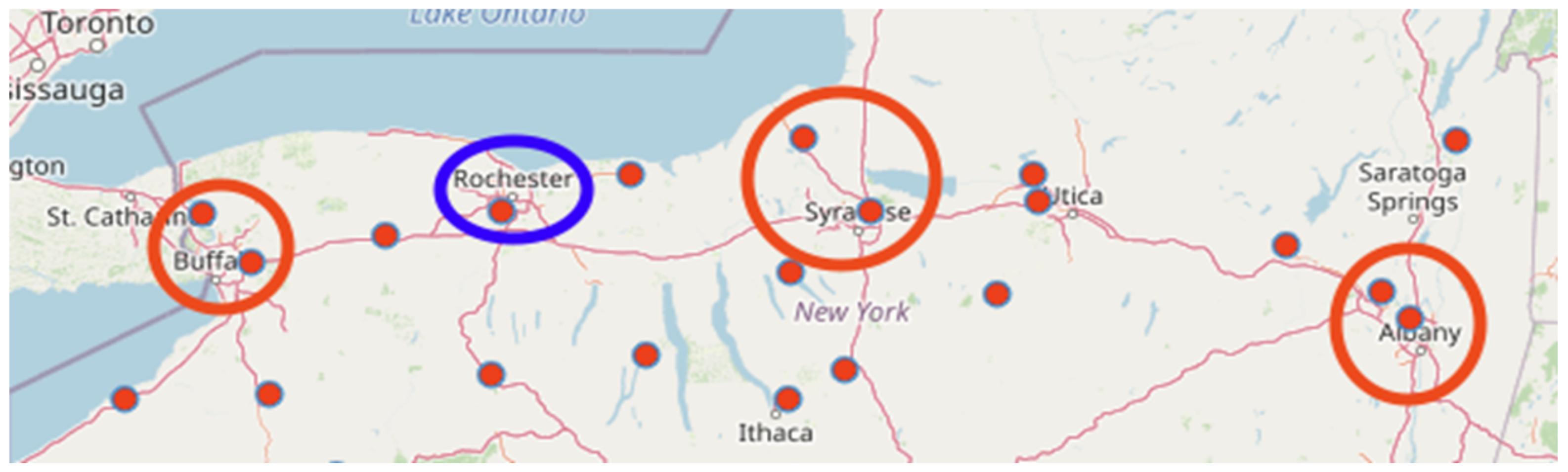
From the aspect of the dataset, we focus on the regional rainfall forecasting in Upstate New York, a geographic region consisting of the portion of New York State lying north of the New York City metropolitan area. Upstate New York historically had sufficient precipitation until recently, with intense drought occurring over the recent years [37]. Our study can benefit the rainfall forecasting for agriculture and economy-related activities in Upstate New York over different catchments. Figure 1 shows the map of weather stations on which the rainfall datasets were collected.

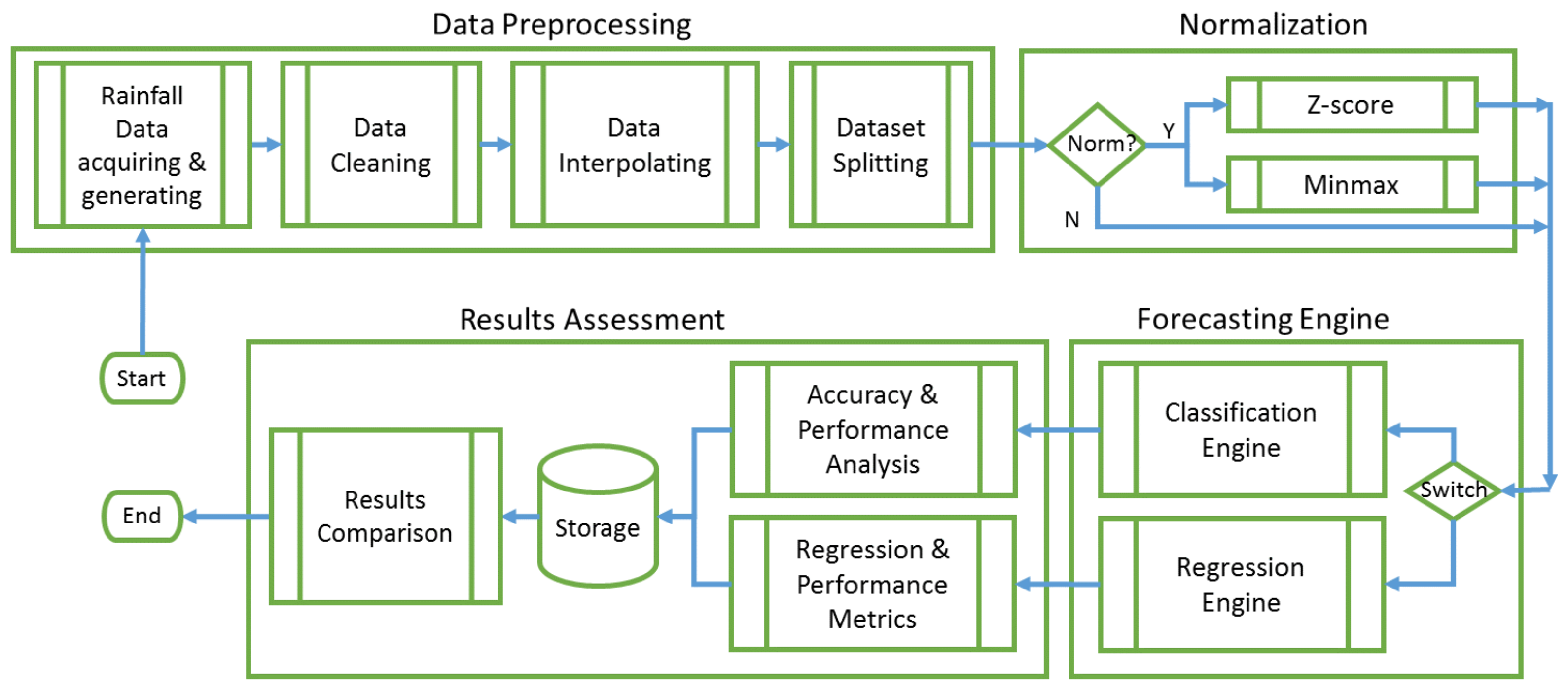
In summary, the contributions of this study are generalized as following thrusts. (1) We proposed a generic computing framework that can integrate a variety of machine learning models as engine options for regional rainfall forecasting in Upstate New York. It can provide a practical open-source framework for modeling rainfall forecasting and benefit the agriculture and related activities in Upstate New York. (2) Relying on the proposed prediction framework, we are able to quantitatively analyze, compare, and evaluate a variety of machine learning algorithms based on the same computing framework and the same datasets. It is superior to the existing literature in depth (quantitative comparison) and width (more algorithms involved). Meanwhile, (3) we integrate the most used normalization methods Z-score and Minmax to investigate the impact of normalization methods on those machine learning algorithms, which is unique over other similar literature.

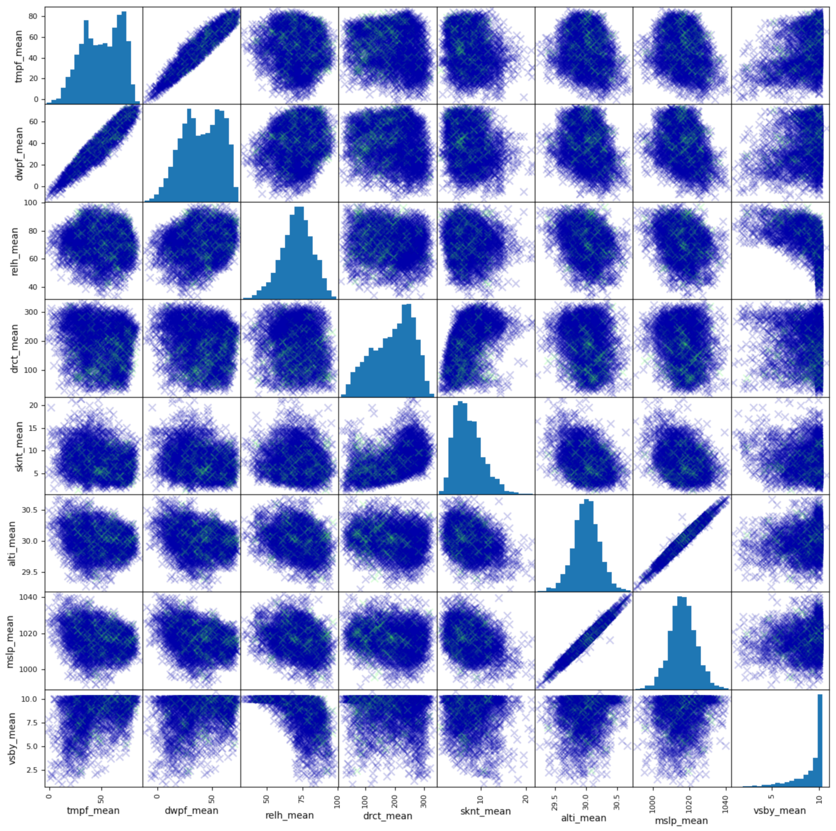
The remaining sections are organized in the following way. In Section 2 we introduce the related work to this study. After that, in Section 3.1 we depict the prototype of the generic computing framework in which a variety of machine learning models are integrated for regional rainfall forecasting. There are also other two important components in Section 3. In Section 3.2 we show the datasets and how they are prepared for the models, and in Section 3.3 we depict those machine learning models and related algorithms that are bagged into the framework. Subsequently, in Section 4 we show the experimental performances of those bagged models in the computing framework for classification and regression. At last, in Section 5 we give the further discussion about the results and conclude the paper.

2. Related Work

As one of the machine learning models, the K-nearest neighbors model has shown a promising performance in climate prediction [38,39,40,41]. For example, Jan et al. applied KNN for climate prediction by using the historical weather data of a region such as rain, wind speed, dew point, and temperature [42]. However, until the recent years starting from 2017, the KNN related methods for rainfall forecasting have drawn more attention from researchers. Huang et al. developed a KNN-based algorithm to offer robustness in the irregular class distribution of the precipitation dataset and made a sound performance in precipitation forecast [43]. However, they did not show the comparison with other advanced machine learning algorithms such as deep learning, limiting its application on the rainfall forecasting. Yang et al. developed an Ensemble–KNN forecasting method based on historical samples to avoid uncertainties caused by modeling inaccuracies [44]. Hu et al. proposed a model that combined empirical mode decomposition (EMD) and the K-nearest neighbors model to improve the performance of forecasting annual average rainfall [45]. A KNN-based hybrid model was used to improve the performance in monthly rainfall forecasting [46].

Like multi-layer perceptrons and radial basis function networks, support vector machines can be used for pattern classification and nonlinear regression. SVM has been found to be a significant technique to solve many classification problems in the last couple of years. Hasan et al. exhibited a robust rainfall prediction technique using Support Vector Regression (SVR) [47]. Support Vector Machine based approaches also have illustrated quite the capability for rainfall forecasting. Support vector regression combined with Singular Spectrum Analysis (SSA) has shown its efficiency for monthly rainfall forecasting in two reservoir watersheds [48]. Yu et al. conducted a comparative study and revealed that a single-mode SVM-based forecasting model can have a better performance than multiple-mode forecasting models [49]. Tao et al. adopted a hybrid method that combined SVM and an optimization algorithm to improve the accuracy of regional rainfall forecasting in India [50].

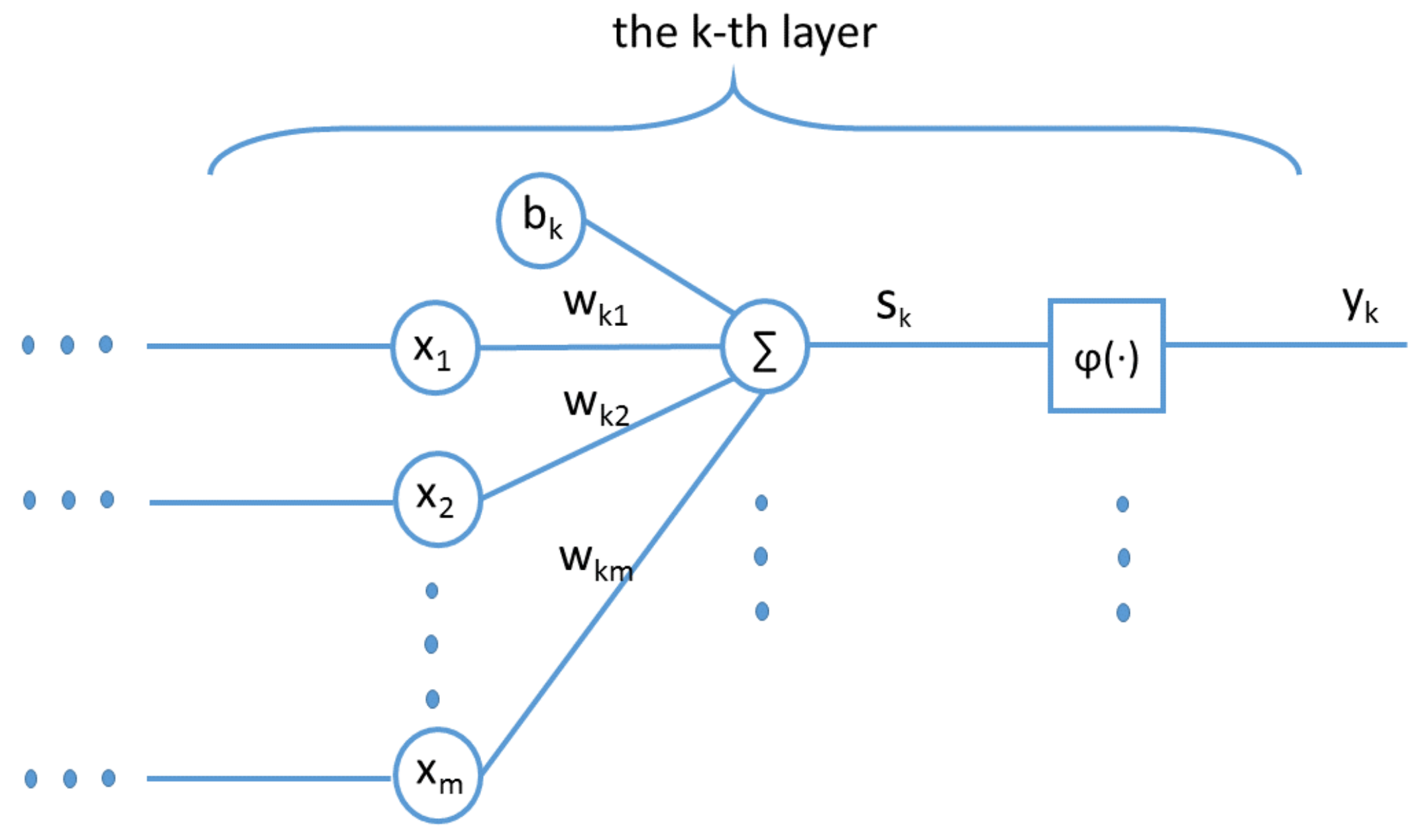
As a type of Artificial Neural Networks (ANN), DNN can emulate the process of the human nervous system and have proven to be very powerful in dealing with complicated problems, such as computer vision and pattern recognition. Moreover, DNN are computationally robust even when input data contains lots of uncertainty such as errors and incompleteness. Such examples are very common in rainfall data.

A pioneer two-dimensional ANN model [51] was used to simulate complex geophysical processes and forecast the rainfall. Howevr, it was limited by many aspects including insufficient neural network configurations and a mathematical rainfall simulation model that was used to generate the input data. More applications of NN models were developed later. Koizumi utilized an ANN model for radar, satellite, and weather-station data together to provide better performance than the persistence forecast, the linear regression forecasts, and the numerical model precipitation prediction [52]. By comparing several short-time rainfall prediction models including linear stochastic auto-regressive moving-average (ARMA) models, artificial neural networks (ANN), and the non-parametric nearest-neighbors method, a significant improvement on those ANN-based models were demonstrated in real-time flood forecasting [53,54]. Luk et al. developed several types of Artificial Neural Networks and revealed that rainfall time series have very short-term memory characteristics [3]. The performance of three Artificial Neural Network (ANN) approaches were evaluated in the forecasting of the monthly rainfall anomalies for Southwestern Colombia [55]. The combination of ANN approaches had demonstrated the ability to provide useful prediction information for the decision-making. A similar case study conducted by Hossain et al. uncovered that the non-linear model ANN can beat multiple linear models in rainfall forecasting in western Australia [56]. Similarly, Jaddi and Abudullah utilized optimization techniques [57] to choose and optimize the weights in neural networks [58]. Hung et al. applied ANN model for real time rainfall forecasting and flood management in Bangkok, Thailand [59].

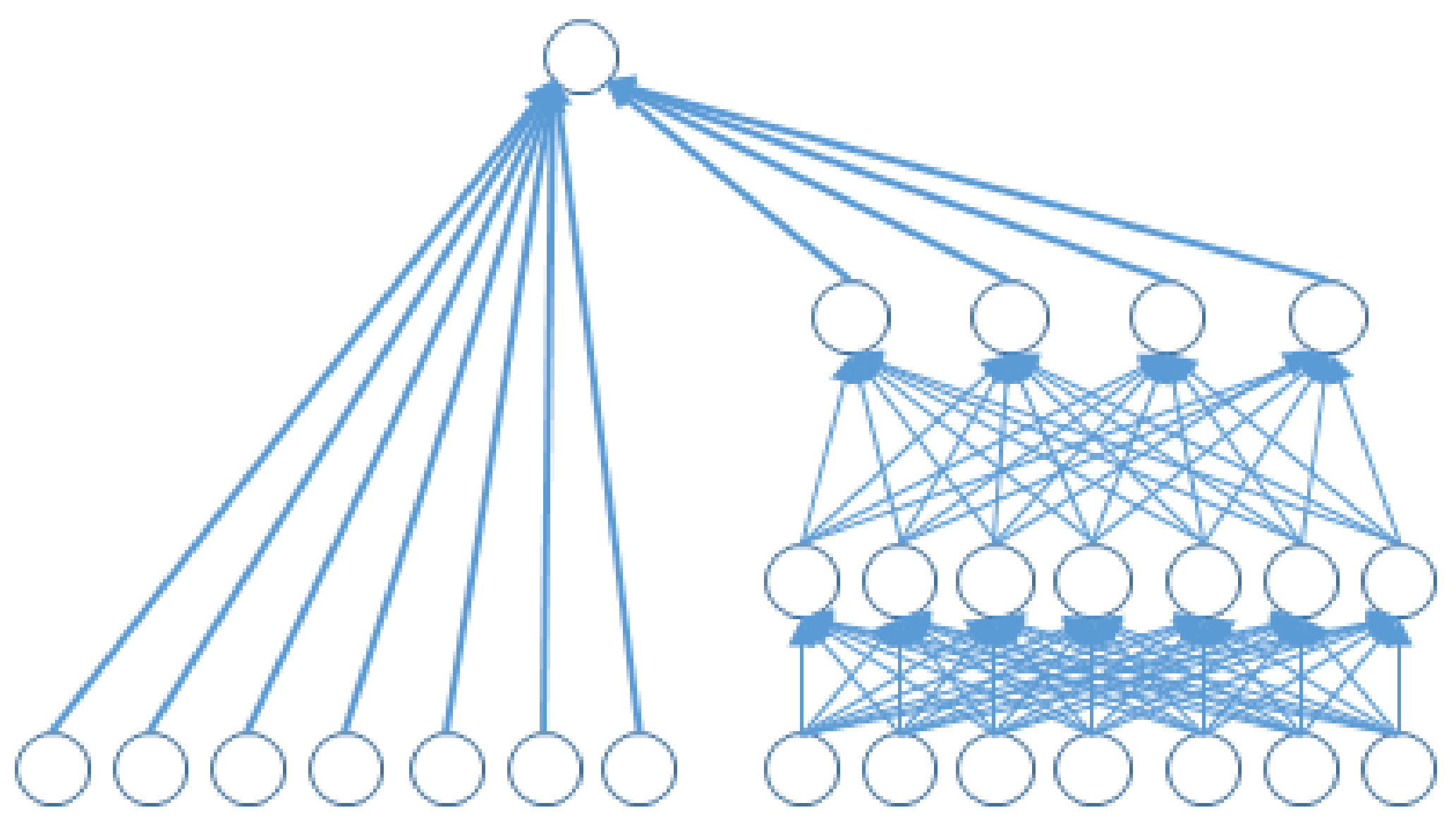
Cheng et al. proposed Wide & Deep Neural Network (WDNN or DWNN) model for recommender systems originally, where it contains two components: wide neural network and deep neural network [60]. The wide neural network (WNN) was designed to effectively memorize the feature interactions through a wide set of cross-product feature transformations. The deep neural network (DNN) was used to better generalize hidden features through low-dimensional dense embeddings learned from the sparse matrix [60]. DWNN has been used in various applications, such as clinical regression prediction for Alzheimer patients [61]. In the latest publication, Bajpai and Bansal analyzed and evaluated three deep learning approaches, one dimensional Convolutional Neutral Network, Multi-layer Perceptron, and Wide Deep Neural Networks for the prediction of regional summer monsoon rainfall in India and found that DWNN can achieve the best performance over the rest two deep learning methods [62].

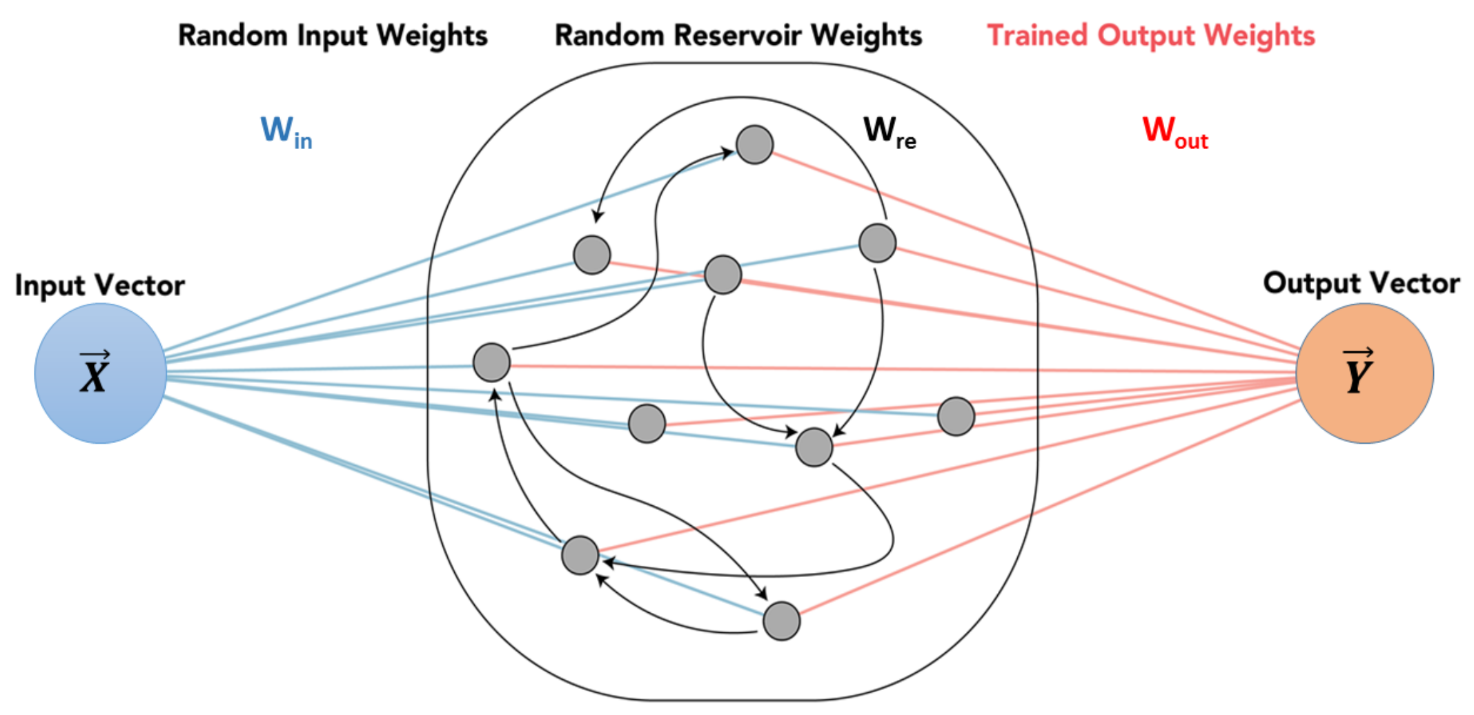
The Reservoir Computing framework has been known for over a decade as a state-of-the-art paradigm for the design of RNN [63]. Among the models of RC instances, the echo state network (ESN) represents a type of the most widely known schemes with a strong theoretical support and various applications [64]. Yen et al. used the ESN and the DeepESN algorithms to analyze the meteorological hourly data in Taiwan and showed that DeepESN was better than that by using the ESN and other neuronal network algorithms [65]. Backpropagation algorithms and Reservoir Computing in Recurrent Neural Networks were adopted to predict the complex spatio-temporal dynamics [66]. An ESN-based method was proposed by Ouyang and Lu to better forecast the monthly rainfall while a SVM regressor was used as a reference for the comparison [67]. Coulibaly utilized Reservoir Computing approach to forecast the Great Lakes water level and achieved the better forecasting performance over other two neural networks including recurrent neural network [68]. A similar approach was used by De Vos to investigate the effectiveness of neural networks in rainfall-runoff modeling [69]. Bezerra et al. took advantage of the characteristic of dynamic behavior modeling in RC and combined RC with trend information extracted from the series for short-term streamflow forecasting, achieving better generalization performance than linear time series models [70].

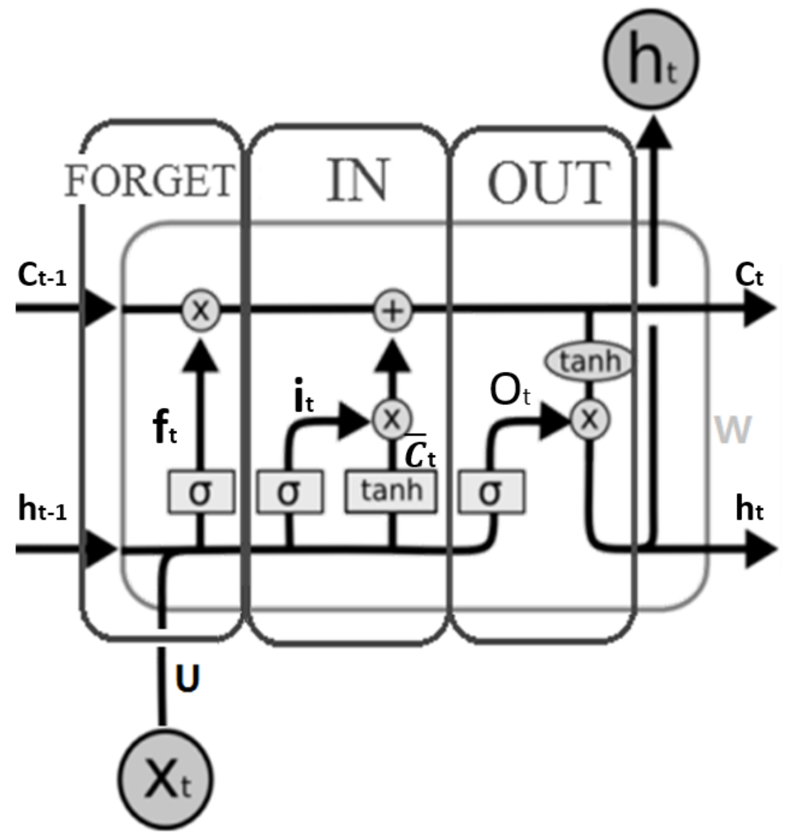
As a type of recurrent neural network (RNN), Long Short-Term Memory neural networks (LSTM) have been studied by many researchers in recent literature. Liu et al. used LSTM to simulate rainfall–runoff relationships for catchments with different climate conditions [71]. The LSTM model then was coupled with a KNN algorithm as an updating method to further boost the performance of LSTM method. LSTM-KNN model was validated by comparing the single LSTM and the recurrent neural network (RNN). Chhetri et al. studied LSTM, Bidirectional LSTM (BLSTM), and Gated Recurrent Unit (GRU), another variant of RNN [72]. LSTM recorded the best Mean Square Error (MSE) score which outperformed the other six different existing models including Linear Regression, Multi-Layer Perceptron (MLP), Convolutional Neural Network (CNN), GRU, and BLSTM. They further modified the model by combining LSTM and GRU to carry out monthly rainfall prediction over a region in the capital of Bhutan.

As an emerging technology, deep learning based methods have embarked as a trend for weather forecasting or rainfall forecasting in recent years [65,73,74,75]. Klemmer et al. utilized Generative Adversarial Networks (GAN) to generate the spatio-temporal weather patterns for the extreme weather event [76]. Hossain et al. employed a deep neural network with Stacked Denoising Auto-Encoders (SDAE) to predict air temperature from historical dataset including pressure, humidity, and temperature data gathered in Northwestern Nevada [77]. Karevan and Suykens developed a 2-layer spatio-temporal stacked LSTM model in an application [78] for regional weather forecasting in 5 cities including Brussels, Antwerp, Liege, Amsterdam, and Eindhoven. A deep LSTM network on the Spark platform was developed by Mittal and Sangwan for weather prediction using historical datasets collected from Brazil weather stations [79]. Qiu et al. elaborated a multi-task model based on convolutional neural network (CNN) to automatically extract features and predict the short-term rainfall from sequential dataset measured from observation sites [80]. Hewage et al. proposed a data-driven model using the combination of long short-term memory (LSTM) and temporal convolutional networks (TCN) for weather forecasting over a given period of time [31].

However, as we discussed in Section 1, most literature were specific and limited to only particular techniques such as deep learning, neural networks, or support vector machine and lacked the quantitative comparison and investigation over a wide range of existing machine learning models. Our study can make up this niche by developing a generic framework based on machine learning models and quantitatively comparing a variety of models through the same computing framework and datasets.

In addition, we also investigated the impact of normalization on machine learning algorithms, as normalization has shown its important impact as part of data representation for feature extraction [81]. The purpose of normalization is to convert numeric values in the dataset to the ranges of values in a common scale without erasing differences or losing significant information. Normalization is also required for some algorithms to model the data correctly [82,83]. Normalization issues have drawn broad attention from researchers in machine learning [84,85,86,87]. For example, batch normalization becomes a technique widely adopted in machine learning modeling [82,88,89]. One of its fundamental impacts is that normalization makes the optimization landscape significantly smoother and it further induces a more predictive and stable behavior of the gradients and results in a faster training [90]. Some experiments were conducted to contrast the performance between normalization and non-normalization [91,92]. However, they involved only a few machine learning algorithms. Our study can make up this niche by integrating the normalization methods to a variety of machine learning models in a generic framework to test the impacts of non-normalization and normalization and the difference between the commonly used normalization methods Z-score and Minmax.

3. Methods

3.1. A Generic Framework

Figure 2 illustrates the generic computing framework for regional rainfall forecasting in Upstate New York. This framework is an abstract software environment that can provide generic functionality and easily launch specific models according to additional needs. The framework contains four main components: precipitation data preprocessing, data normalization, forecasting engines, and results assessment, as shown in Figure 2.

Data Preprocessing: In the first step of data preprocessing, a rainfall data acquiring and generating process is conducted. We have developed an automatic data acquiring tool to acquire and generate data from the online data source. After data acquiring and generating, raw data are fed further to three parts: cleaning, interpolating, and splitting. There are some empty items and some duplicates existing in the raw datasets. We delete those empty and duplicated items. Data interpolating is used to handle many empty values spread around the entire dataset. We calculate the average value from its chronicle neighbors and interpolate it as the estimated value. As a necessary step for training and testing in machine learning models, we adopt 70/30 ratio in dataset splitting to meet the need. The detailed process is described in Section 3.2.

Data Normalization: Two important normalization methods, Z-score and Minmax, are used to evaluate the impact of normalization and non-normalization in the framework. The Z-score value $z_i$ is calculated in terms of Equation (1):

$$z_i=\frac{x_i-\mu }{\delta },$$

(1)

where $x_i$ is the i-th observed value, $\mu$ is the mean of all values in the variable and $\delta$ is the standard deviation in the variable. The Minmax value $m_i$ is computed in terms of Equation (2):

$$m_i=\frac{x_i-min}{max-min},$$

(2)

where $min$ is the minimum value and $max$ is the maximum value in the variable respectively.

Forecasting Engines: The computing framework provides the options of machine learning models and algorithms for either classification or regression. The technical details of models and algorithms are described in Section 3.3.

Result Assessment: Different assessment metrics are used for evaluating classification and regression respectively. In classification, accuracy is the most used to measure the classifier’s performance, which can greatly manifest the capability of predictive models. In regression, the coefficient of determination ($R^2$), Mean Square Error (MSE), Root Mean Square Error (RMSE), and Pearson Correlation Coefficient (Pcc) are adopted to measure the fitness of a regression model to the dataset. After the experimental results are obtained and saved in the local storage, a comparison based on these assessment metrics will be conducted.

3.2. Data Preprocessing

The data was obtained from Iowa State University’s Iowa Environmental Mesonet which has a portal to download Automated Surface Observing System (ASOS) data (available online: https://mesonet.agron.iastate.edu/ASOS/, accessed on 10 May 2021) from weather stations around the US [93]. Four regional data sets were collected as illustrated in Figure 1: Rochester data came from the ROC weather station; Buffalo data came from the BUF and IAG weather stations; Syracuse data came from the SYR and FZY weather stations; and Albany data came from the ALB and SCH weather stations. We designed an online tool that enables us to collect 11 years of historical hourly weather data automatically from the locations we needed for our project. The features/variables of the climatic data that we collected from each location and used for this study were: hourly precipitation in inches (p01i), temperature in fahrenheit (tmpf), dew point in Fahrenheit (dwpf), relative humidity as a percent (relh), wind direction in degrees from North (drct), wind speed in knots (sknt), Pressure altimeter in inches (alti), sea level pressure in millibar (mslp), and visibility in miles (vsby). The regression target was the precipitation in inches for the next hour.

Take the Rochester Dataset as an example, the plot matrix shown in Figure 3 virtually indicates the relationships between the numeric features. There are two sets of features with clear linear correlations, that being Temperature and Dew Point as well as Pressure and Sea Level Pressure. Temperature and Dew point are commonly used in calculating Heat Index, so it makes sense that they are strongly related. The two different measurements of air pressure seem nearly identical but as you can see in the chart, they are positively correlated but not exactly the same. Besides the two sets of strongly correlated features, the other features present a more complicated relationship. In this plot matrix, the data points in which the following day had precipitation are marked in green while the rest of the data points are blue.

After the raw dataset was acquired, it was grouped into hour intervals starting with 0 on 1 January 2010, at midnight. These groups were averaged into a single row for all the features except p01i. That is one hour precipitation for the period from the observation time to the time of the previous hourly precipitation reset. p01i is specifically the accumulated precipitation within an hour so the max was taken for each group for the p01i feature. All missing p01i values were set to 0. The decision was made after looking at random hour intervals whose p01i value was missing and cross-referencing that time frame with Available online: Weather.com (accessed on 10 May 2021). For the rest of the features, missing values were interpolated from their previous and future hour interval values.

From the cleaning and interpolating, two separate datasets were created. One dataset had only data from Rochester (ROC). The second dataset had the mixed data from Rochester as well as corresponding data from Buffalo, Syracuse, and Albany (Mixed or ROC + BUF + SYR + ALB). The second dataset was created by performing a left join of the Rochester data with a union of the rest of the data. Intervals where Rochester had data but the others did not, had their values interpolated by the same method that was used to previously remove missing values.

At this point in the data’s life, two separate versions of the two datasets were made: one for classification where an interval’s target was a binary 0/1 of whether the next interval’s p01i value exceeded 0.01 inches; another for the regression where an interval’s target was the next interval’s p01i value. According to the categories in hydrology, hourly rainfall in 0.01 inches is a very small amount that can be ignored and eliminating the smallest of the values also can reduce noise.

For both ROC and Mixed datasets, a Minmax normalized version, a Z-score normalized version, and a non-normalized version were made. This resulted in 6 datasets for classification and 6 datasets for regressors. For all the classifiers and regressors, the 11 years of hourly data was split into 70% for training and 30% for testing. For all except LSTM, the split was made by shuffling the data by a given random state and split after shuffling. In the cases where random states were used to shuffle the data, the random states considered were 0, 42, and none (0 and none are the first values that can be chosen but 42 is a special choice made by many, which comes from the book The Hitchhiker’s Guide to the Galaxy). The use of none for a random state indicates that the data was not shuffled before the split.

3.3. Models and Algorithms

A set of algorithms of SVM, KNN, DNN, WNN, DWNN, RC, and LSTM, are used to forecast regional rainfall. These models and algorithms are provided as forecasting engines in our integrated framework. We describe these models and algorithms as follows.

3.3.1. K-Nearest Neighbors

KNN algorithm is a robust method that can approximate its outcome by averaging the observations in the same neighborhood. The neighborhood is determined by the distance between the observations and the input point [40]. The distance can be measured by many methods such as Manhattan distance, Euclidean distance, and Minkowski distance. Euclidean distance is calculated as the square root of the sum of the squared differences between a new point x and an existing point $x^{\prime }$. Equation (3) shows the distance measurement:

$$D(x,x^{\prime })=\sqrt{\sum _{i=1}^n{(x_i-x_i^{\prime })}^2},$$

(3)

where i is the i-th feature of nodes x and $x^{\prime }$. KNN can be used for both classification and regression. In KNN regression, the output value is the average of the values of k nearest neighbors. In KNN classification, the output value is the most common class among k nearest neighbors. The value of k can be chosen manually or using cross-validation to select the size that minimizes the mean-squared error or maximize the accuracy.

3.3.2. Support Vector Machine

Support vector machine (SVM) or support vector regressor (SVR) aims to find the hyperplane [94]. The difference between SVM and SVR is that one segregates the nodes for classification while the other finds the decision boundary along with hyperplane and has the least error rate to fit the model. The hyperplane in a SVM is shown in Equation (4):

$$y=w^T·x+b,$$

(4)

where x is a vector of features, w is a vector of normalized direction to the hyperplane, and b is a form of threshold.

SVM has a powerful way to project dataset into higher dimension by using kernels. A common kernel function K can be linear such as dot product, or non-linear such as Radial basis function kernel (rbf) as shown in Equation (5):

$$K(x_1,x_2)=e^{-\gamma {∥x_1-x_2∥}^2},$$

(5)

where $\gamma$ is a parameter for rbf kernel, and ${∥x_1-x_2∥}^2$ is the Euclidean distance. In this study, we utilize four kernels: linear kernel, polynomial kernel, rbf/Gaussian kernel, and sigmoid kernel.

3.3.3. Deep Neural Network

Artificial neural Networks are generalized models of biological neuron systems. Deep neural networks are a type of artificial neural network, which contains a number of layers and can massively distribute processing over layers of neurons or perceptrons [56]. Each neuron or perceptron is the elementary unit containing a simple linear summing function and an activation function as shown in Figure 4. The summing function is shown in Equation (6):

$$s_k=\sum _{j=1}^m{w}_{kj}{x}_j+b_k,$$

(6)

where k denotes the identifier of the k-th layer, $x_j$ is the input of node j, and $b_k$ is the bias of layer k. The sigmoid function is often used as an activation function as shown in Equation (7):

$$y_k\left(s\right)=\phi \left(s_k\right)=\frac{1}{1+e^{-s_k}}.$$

(7)

3.3.4. Wide Neural Network

The core of a wide neural network is a generalized linear model as shown in Equation (8):

$$y=w^{T}x+b,$$

(8)

where x is a vector of d features, w is the weights or parameters, and b is the bias. The d feature set may be raw input features or transformed features. A cross-product transformation is utilized to capture the interactions between the binary features, which adds a non-linear factor to the generalized linear model, as shown in Equation (9):

$${\varphi }_k\left(x\right)=\prod _{i=1}^d{x}_i^{c_{ki}},c_{ki}\in \{0,1\},$$

(9)

where $c_{ki}$ is 1 if the i-th feature is part of the k-th transformation ${\varphi }_k$ and 0 if the i-th feature is not part of the k-th transformation ${\varphi }_k$. The generalized linear models with cross-product feature transformations can memorize these exception rules with much fewer parameters [60].

3.3.5. Wide and Deep Neural Network

The Wide and Deep Neural Network is composed of a wide neural network and a deep neural network using a weighted sum of their output log odds as the prediction and a common logistic loss function for a joint training [60]. In the joint training, the wide component uses a small number of cross-product feature transformations to complement the weaknesses of the deep neural network.

The deep component is a feed-forward neural network, as shown on the right side of Figure 5 while the wide component is a linear model based neural network, as shown on the left side of Figure 5. The low-dimensional vectors are fed into the hidden layers of a neural network in the forward pass according to Equation (10):

$$y_{k+1}=\phi (w_k{y}_k+b_k),$$

(10)

where k is the layer number and $\phi$ is the activation function, $y_k$, $w_k$, and $b_k$ are the output, model weights, and bias in the k-th layer respectively.

3.3.6. Reservoir Computing

The reservoir computing (RC) framework consists of three layers: input layer, reservoir layer, and output layer, as depicted in Figure 6.

The input layer consists of the input weights for each reservoir perceptron. It is a randomly generated matrix with values uniformly distributed between 0 and $\delta$, where $\delta$ is a scaling factor that allows the reservoir computing to adjust the methods for training data of various sizes. The input layer matrix of the weights is denoted as $W_{in}$.

The reservoir layer is where the actual recurrent neural network is held. The current i-th state of the reservoir is described as a vector, referenced as $\overrightarrow{r}\left(i\right)$. The perceptron weights are described by a connectivity/adjacency matrix, $W_{re}$. This matrix is an Erdös-Rényi randomly generated matrix. The eigenvalues of the matrix are normalized, and scaled by a factor, $\rho$, known as the spectral radius that determines how the reservoir adapts to changing dynamics. The activation function for the reservoir is given in Equation (11):

$$\overrightarrow{r}\left(i\right)=tanh[\overrightarrow{r}(i-1)\times W_{re}+\overrightarrow{X}\left(i\right)\times W{}_{in}],$$

(11)

where $\overrightarrow{r}(i-1)\times W_{re}$ represents the reservoir’s feedback and is what allows the reservoir to attach to new input vectors and the $\overrightarrow{X}\left(i\right)$ represents the vector of new input to the reservoir. The input term and activation function may vary in different implementations of reservoir computing [63].

The output layer is how a prediction is obtained from the reservoir. The output layer is a (# of perceptrons) × ( # of classes) matrix, referred to as $W_{out}$. The output is obtained by Equation (12):

$$output=\overrightarrow{r}\left(i\right)\times W{}_{out}.$$

(12)

3.3.7. Long Short Term Memory

The LSTM network accepts the output of the previous moment, the current system state, and the current system input. It then updates the system status through the input gate, the forget gate, and the output gate. Then it finally outputs the result [95]. As shown in Figure 7, the forget gate is $f\left(t\right)$, the input gate is $i\left(t\right)$, the output gate is $o\left(t\right)$, and the cell state is $C_t$.

According to the network structure in Figure 7, the forget gate decides the information forgotten and controls the transfer of information from the previous time as shown in Equation (13):

$$f_t=\delta (U_f{x}_t+W_f{h}_{t-1}),$$

(13)

where $U_f$ and $W_f$ are the weights of the recurrent and input connections accordingly in the forget gate and $\delta$ is an activation function such as sigmod or hyperbolic tangent.

The input gate determines the current time system input, which acts in front of the forget gate to supplement the latest memory of the network, as shown in Equation (14):

$$i_t=\delta (U_i{x}_t+W_i{h}_{t-1}),$$

(14)

where $U_i$ and $W_i$ indicates the weights from the recurrent and the input connections accordingly in the input gate.

The current cell memory $C_t$ is defined in Equation (15):

$$C_t=f_t{C}_{t-1}+i_t\overline{C_t},$$

(15)

where $\overline{C}$ is shown in Equation (16):

$$\overline{C_t}=tanh(U_c{x}_t+W_c{h}_{t-1}),$$

(16)

where $U_c$ and $W_c$ are the weights of the connections to $\overline{C}$ accordingly.

The output gate $O_t$ is shown in Equation (17):

$$O_t=\delta (U_o{x}_t+W_o{h}_{t-1}),$$

(17)

where $\delta$ is an activation function and $U_o$ and $W_o$ are the weights of the connections to the output gate accordingly. The current cell output $h_t$ is shown in Equation (18):

$$h_t=tanh\left(C_t\right)O_t.$$

(18)

Bidirectional LSTM and Gated Recurrent Unit (GRU) are viewed as variants of LSTM. Bidirectional LSTM can receive the input from two directions: one is from past to future and one is from future to past, which is different from unidirectional LSTM. GRU is similar to a LSTM model but it lacks an output gate. Therefore, GRU has fewer parameters than LSTM, and has demonstrated better performance in relatively small datasets [96].

4. Results Assessment

4.1. Running and Tuning

The KNN, SVM, Linear, and RC models for rainfall forecasting were implemented based on SKLearn libraries, running on M1 Mac (Apple M1 chip, 8-core CPU, 8-core GPU, 16-core Neural Engine, 16.0 GB RAM, 1TB SSD HD). The DNN, WNN, DWNN, and LSTM models for rainfall forecasting were implemented based on Tensorflow libraries, running on Intel Xeon CPU (E3-1240 V2 @ 3.40 GHz, 16.0 GB RAM, NVIDIA GeForce GTX 1070 GPU, TOSHIBA HDWD130 3TB Sata 6 Gbs 7200RPM). The software Github package as well as the datasets can be found online: https://github.com/Oeathus/ANNSIM21 (accessed on 10 May 2021).

To ensure a fair comparison between the models, each model was given the same data as all other models. Also, where a parameter was required that was specific to any of the models, like layers for DNN and DWNN or Kernels for SVM and SVR, there was a loop made to test multiple values for that model. In the case of SVM and SVR, there were only four possible values for the parameter so they were all tried. For models whose parameter had a virtually unlimited set of possible values, like the number of layers for DNN or DWNN, we tried multiple values spaced apart in such a way to try and capture the best that could be done in a reasonable amount of time. For models that could train and infer quickly, more values were tested and for models that took more time to train and infer, fewer values were tested. With that said, for all but the Linear Regressor, WNN Classifier, and WNN Regressor, only the main parameter was different. For the aforementioned models, there was no main defining parameter. Outside of the one different parameter, all other settings such as normalization, random state, and features were the same for all models in each combination of settings.

4.2. Classification

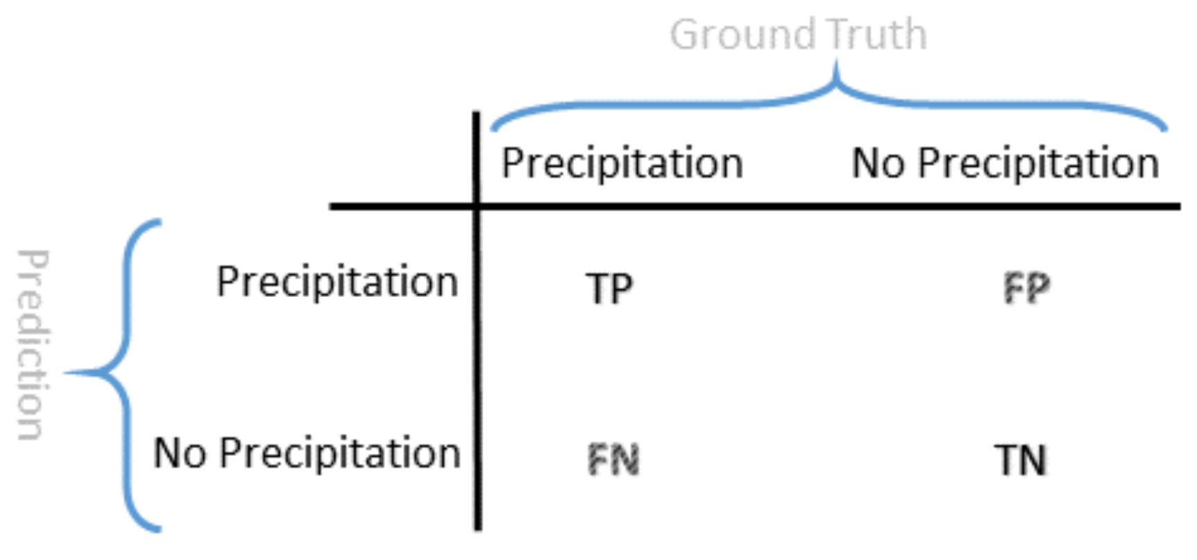
Accuracy is the metric to measure the classifier’s performance. It is expressed in Equation (19):

$$Accuracy=\frac{TP+TN}{TP+TN+FP+FN},$$

(19)

where TP is true positive, TN is true negative, FP is false positive, and FN is false negative according to the confusion matrix shown in Figure 8.

KNN: Six datasets were crossed with the 3 different random seeds for a total of 18 forms of data. These 18 forms were iterated through a KNN Classifier 25 times to find the best n_neighbor value. After 450 iterations the best accuracy was 96.09% which was obtained from the Rochester, Buffalo, Syracuse, and Albany dataset, normalized by Z-score, a random state of 0, and 9 n_neighbors.

SVM: There were 72 unique Support Vector Machine Classifiers by training against the cross of 6 premade datasets, 4 kernels, and the same 3 random states as before. The best accuracy for SVM, and ultimately the best accuracy for all classifiers, was 96.22% obtained from the ROC + BUF + SYR + ALB, normalized with Z-score, using 0 as random state and the rbf kernel.

DNN: 126 DNN Classifiers were tested and used by training against the cross of the 6 premade datasets, 7 different amounts of hidden layers, and the 3 random states used from before. The 7 different hidden layers were: 2, 3, 4, 5, 10, 20, and 30 layers. Each of the hidden layers had the number of inputs equal to the number of features which for the ROC datasets was 9 and for the ROC + BUF + SYR + ALB there were 36 inputs at each hidden layer. The best accuracy for DNN was 94.81% obtained from the ROC dataset only, normalized with Z-score, using 42 as random state and with 10 hidden layers.

WNN: There were 18 unique WNN Classifiers by training against the cross of the 6 premade datasets and the 3 random states used from before. The best accuracy for WNN was 95.91% obtained from the ROC + BUF + SYR + ALB, normalized with Z-score, using 0 as random state.

DWNN: There were 126 unique DWNN Classifiers by training against the cross of the 6 premade datasets, 7 different amounts of hidden layers for the deep aspect, and the 3 random states used from before. The 7 different hidden layers were: 2, 3, 4, 5, 10, 20, and 30 layers. Each of the hidden layers had the number of inputs equal to the number of features which for the ROC datasets was 9 and for the ROC + BUF + SYR + ALB there were 36 inputs at each hidden layer. The best accuracy for DWNN was 95.74% obtained from the ROC + BUF + SYR + ALB, normalized with Z-score, using None as random state and with 10 hidden layers.

RCC: Reservoir Computing Classifier was investigated because, in a previous investigation of daily values, RCC had the highest accuracy. For RCC, six datasets were crossed with the same 3 random states as before and crossed again with 6 different sizes of the reservoir; 50, 100, 200, 400, 600, 1000. The result of these crosses was 108 unique data forms to train with. The best accuracy was 95.81% which was obtained from the Rochester only dataset, normalized by Z-score, a random state of 42, and a reservoir size of 1000.

LSTM: There were 12 unique LSTM Classifiers by training against the cross of the 6 premade datasets, and 2 different sequence lengths. Random states were not used for LSTM as it depends on chronologically consecutive rows of data. The two sequence lengths considered were 3 previous rows of data and 7 previous rows of data. The best accuracy for LSTM was 94.82% obtained from the ROC + BUF + SYR + ALB, normalized with Minmax, using a sequence length of 3.

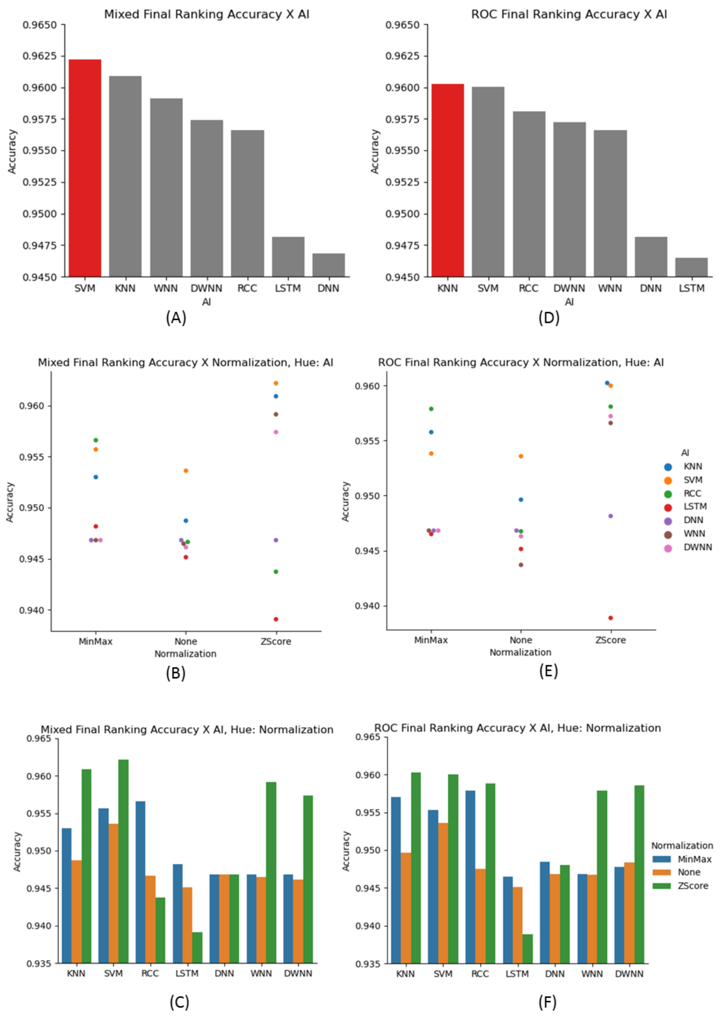
Overall: Both SVM and KNN classifiers performed the best. Figure 9A,D show all of the best accuracies for each of the classification methods used in the mixed and ROC datasets. The plotting for this ranking was zoomed into the accuracy range of 94.5–96.5% to better show the differences between the methods. A further examination of the ranking with the normalization data is shown in Figure 9C,F. In almost every case except for LSTM, the best normalization method was Z-score. It can also be seen that in many cases the non-normalized version of the data performed measurably worse than its Z-score counterpart. The groups of (B,E) and (C,F) are derived from the same results. However, Figure 9B,E show another way to highlight the performance in regards to normalization.

4.3. Regression

Being that accuracy is not measured the same for regressors the metrics recorded were the coefficient of determination ($R^2$), the root of the mean-squared error (RMSE), the mean-squared error (MSE), and Pearson Correlation Coefficient (Pcc). The data used to train and test the regressors in this section was a subset of the data used for the classifiers such that all rows targets were above 0.01, that target being the next hours p01i value (precipitation inches). This decision was made after an initial investigation with the full dataset resulted in much poorer performances. This was likely due to the overwhelming ration of non-precipitation hours (outliers) compared to precipitation hours.

$R^2$, MSE, RMSE, and Pcc are expressed in Equations (20)–(23) respectively:

$$R^2=1-\frac{{\sum }_i{(y_i-f_i)}^2}{{\sum }_i{(y_i-\overline{y})}^2},$$

(20)

$$MSE=\frac{1}{n}\sum _{i=1}^n{(y_i-f_i)}^2,$$

(21)

$$RMSE=\sqrt{\frac{1}{n}\sum _{i=1}^n{(y_i-f_i)}^2},$$

(22)

$$Pcc=\frac{{\sum }_{i=0}^n(y_i-\overline{y})(f_i-\overline{f})}{\sqrt{{\sum }_{i=0}^n{(y_i-\overline{y})}^2}\sqrt{{\sum }_{i=0}^n{(f_i-\overline{f})}^2}},$$

(23)

where $y_i$ is the observed i-th data, $\overline{y}$ is the mean of the observed data, $f_i$ is the modeled value, and $\overline{f}$ is the mean of the modeled values. $R^2$ gives the measurement to what extent the estimation model fits the dataset; MSE shows the quantitative difference between the observed and estimated values; RMSE lowers the magnitude of MSE; and Pcc explains the correlation of the observed data and the predictive model. These four metrics have been widely used in the most related literature.

4.3.1. KNN Regressor

Six datasets were crossed with the same 3 random states as before to make 18 unique forms of data and then each of those 18 was run through a KNN Regressor 1000 times to find the n_neighbor parameter that resulted in the best $R^2$ metrics. The dataset that had the best $R^2$, 0.181718, was the Rochester, Buffalo, Syracuse, and Albany dataset, normalized using Z-score, using None for random state, and with an n_neighbors value of 57. This dataset also had the best MSE and RMSE, 0.005819 and 0.076282. The dataset that had the best Pearson correlation coefficient score, 0.445571, was the Rochester, Buffalo, Syracuse, and Albany dataset, normalized using Z-score, using 42 for random state, and with an n_neighbors value of 37.

Table 1. Top 2 best metric performers in KNN regressor.

Dataset	Norm.	Random	Neighbor	${\mathit{R}}^2$	MSE	RMSE	Pcc
Mixed	Z-score	None	57	0.181718	0.005819	0.076282	0.428720
Mixed	Z-score	42	37	0.179490	0.009653	0.098247	0.445571
ROC	Z-score	None	53	0.151876	0.006031	0.077660	0.392005
ROC	Z-score	42	44	0.136763	0.010155	0.100773	0.376142

shows the top 2 best metric performers in KNN regressor for each dataset source.

4.3.2. Linear Regressor

Six datasets were crossed with the same 3 random states as before and run through a linear regression model. The best metrics were obtained from the Rochester, Buffalo, Syracuse, and Albany dataset, with a random state of None. Because this is a linear regression, the normalizations all yield the same results when the other settings are the same. Those values were $R^2$ = 0.173853, Pcc = 0.418374, MSE = 0.005875, and RMSE = 0.076648.

Table 2. Top 2 best metric performers in Linear regressor.

Dataset	Norm.	Random	${\mathit{R}}^2$	MSE	RMSE	Pcc
Mixed	None	None	0.173853	0.005875	0.076648	0.418374
Mixed	Z-score	None	0.173853	0.005875	0.076648	0.418374
ROC	Z-score	None	0.152275	0.006028	0.077642	0.390999
ROC	None	None	0.152275	0.006028	0.077642	0.390999

shows the top two performing Linear Regression Models and their respective performance metrics for each dataset source. Note that the normalizations do not affect the $R^2$ for the Linear Regressor so that for Mixed or ROC dataset we can put any normalization as they all have the same metrics through the experimental results.

4.3.3. SVM Regressor

Six datasets were crossed with the same 3 random states as before and crossed again with the 4 different kernel options: linear, poly, rbf, and sigmoid. This resulted in 72 data forms that were run through the support vector regressor.

Table 3. Top 2 best metric performers in SVR.

Dataset	Norm.	Kernel	Random	${\mathit{R}}^2$	MSE	RMSE	Pcc
Mixed	Z-score	rbf	42	0.036320	0.011337	0.106474	0.380177
Mixed	Minmax	linear	None	invalid	0.009003	0.094882	0.408546
ROC	None	sigmoid	42	invalid	0.012855	0.113380	0.168737
ROC	Minmax	poly	None	invalid	0.009645	0.098208	0.407548

shows the best performers in each metric for each source. The best $R^2$, 0.036320, came from the Rochester, Buffalo, Syracuse, and Albany dataset, normalized with Z-score, using the rbf kernel, and with a random state of 42. The best Pearson correlation coefficient score, 0.408546, came from the Rochester, Buffalo, Syracuse, and Albany dataset, normalized with MinMax, using the linear kernel, and with a random state of None. However, SVR did not perform well on ROC dataset where the invalid values were calculated in $R^2$. Table 3 shows the top 2 best performers in SVR including the invalid values in $R^2$. It shows that SVM does not perform well in regression tasks.

4.3.4. DNN Regressor

In total, there were 126 DNN Regressors were trained against the cross of the 6 premade datasets, 7 different amounts of hidden layers, and the 3 random states used from before. Seven different hidden layers were: 2, 3, 4, 5, 10, 20, and 30 layers. Each of the hidden layers had the number of inputs equal to the number of features which for the ROC datasets was 9 and for the ROC + BUF + SYR + ALB there were 36 inputs at each hidden layer.

Table 4. Top 2 best metric performers in DNN regressor.

Dataset	Norm.	Layers	Random	${\mathit{R}}^2$	MSE	RMSE	Pcc
Mixed	Minmax	3	None	0.021768	0.006956	0.083405	0.215921
Mixed	Z-score	30	42	Invalid	0.011765	0.108465	0.290540
ROC	Minmax	4	42	0.036257	0.011338	0.106478	0.240040
ROC	Minmax	2	None	0.033795	0.006871	0.082891	0.214836

shows the best two performers in each dataset. The best $R^2$, 0.036257, came from the Rochester only dataset, normalized with Minmax, using 4 hidden layers, and with a random state of 42. The best Pearson correlation coefficient metric, 0.290540, came from the mixed dataset, normalized with Z-score, using 30 hidden layers, and with a random state of 42. The best MSE and RMSE, 0.006871 and 0.082891, came from the Rochester only dataset, normalized with Minmax, using 2 hidden layers, and with a random state of None. Even though we used 30 layers deep neural network, the best performer of $R^2$ in ROC dataset was obtained from the normalization with Minmax, using 4 hidden layers, and a random state of 42.

4.3.5. WNN Regressor

Similarly to the WNN Classifier, there were 18 unique WNN Classifiers by training against the cross of the 6 premade datasets and the 3 random states used from before. For each of the measured metrics there were different models that performed best.

Table 5. Top 2 best metric performers in WNN regressor.

Dataset	Norm.	Random	${\mathit{R}}^2$	MSE	RMSE	Pcc
Mixed	Minmax	0	0.121694	0.008829	0.093963	0.354666
Mixed	Minmax	None	0.099783	0.006402	0.080010	0.415068
ROC	Z-score	None	0.148975	0.006052	0.077793	0.387437
ROC	Minmax	None	0.139087	0.006122	0.078244	0.376594

shows the best performers in each metric. The best $R^2$, MSE, and RMSE (0.148975, 0.006122, 0.078244 respectively), came from the ROC dataset, normalized with Z-score, and with a random state of None. The best Pearson correlation metric, 0.415068, came from the mixed dataset, normalized with Minmax, and with a random state of None.

4.3.6. DWNN Regressor

Similarly to the DNN Regressor, 7 different hidden layers were: 2, 3, 4, 5, 10, 20, and 30 layers.

Table 6. Top 2 best metric performers in DWNN regressor.

Dataset	Norm.	Layers	Random	${\mathit{R}}^2$	MSE	RMSE	Pcc
Mixed	Z-score	20	42	0.181974	0.009623	0.098098	0.426754
Mixed	Z-score	30	42	0.181682	0.009627	0.098116	0.428402
ROC	Z-score	20	None	0.156510	0.005998	0.077448	0.396452
ROC	Z-score	10	None	0.155902	0.006003	0.077476	0.395922

shows the best performers in each metric for each source. The best $R^2$ for the mixed datasets, 0.181974, came from the mixed dataset, normalized with Z-score, using 20 hidden layers, and with a random state of 42. The best $R^2$ for the ROC datasets, 0.156510, was obtained from the Rochester only dataset normalized with Z-score, using 20 hidden layers, and a random state of None.

4.3.7. LSTM Regressor

There were 48 LSTM regressors in total by training against the cross of the 6 premade datasets, and 8 different sequence lengths. Random states were not used for LSTM as it depends on chronologically consecutive rows of data. The 8 sequence lengths considered were 3, 5, 7, 9, 12, 24, 36, and 48 previous rows of data.

Table 7. Top 2 best metric performers in LSTM regressor.

Dataset	Norm.	Sequence	${\mathit{R}}^2$	MSE	RMSE	Pcc
Mixed	Minmax	12	0.093923	0.006489	0.080555	0.310783
Mixed	None	12	0.072728	0.006641	0.081492	0.272889
ROC	None	5	0.099439	0.006424	0.080149	0.318826
ROC	None	48	0.089427	0.006539	0.080865	0.307474

shows the results of the two best performing LSTM regressors over two datasets. The best $R^2$, MSE, and RMSE came from the same model, using the Rochester dataset, not normalized, and using a sequence length of 5. Those values were $R^2$ = 0.099439, MSE = 0.006424, and RMSE = 0.080149. The best Pearson correlation coefficient, 0.318826, came from the Rochester dataset, non-normalized, and using a sequence length of 5. From the mixed dataset, the regressor with highest $R^2$ obtains the lowest MSE and RMSE and the highest Pcc.

4.3.8. LSTM Bi-Direction

The Bidirectional regressor models used the same settings as the LSTM regressor models, so 48 unique Bidirectional regressors were examined with 8 different sequence steps and the maximum length of previous sequence steps of 48.

Table 8. Top 2 best metric performers in LSTM Bi-direction regressor.

Dataset	Norm.	Sequence	${\mathit{R}}^2$	MSE	RMSE	Pcc
Mixed	Minmax	3	0.067292	0.006645	0.081519	0.295810
Mixed	Minmax	7	0.061097	0.006706	0.081889	0.285112
ROC	Minmax	12	0.092928	0.006496	0.080599	0.320603
ROC	None	12	0.085119	0.006552	0.080945	0.311874

shows the results of the two best performing LSTM regressors. The best $R^2$, MSE, RMSE, and Pcc in the Rochester dataset came from the same regressor, normalized using Minmax and using a sequence length of 12. Those values were $R^2$ = 0.092928, MSE = 0.006496, and RMSE = 0.080599. The best $R^2$, MSE, RMSE, and Pcc in the mixed dataset also came from the same regressor that was normalized using Minmax and using a sequence length of 3.

4.3.9. GRU Regressor

The GRU regressor models used the same settings as the LSTM and Bidirectional regressor models, so 48 unique GRU regressors were examined with the maximum sequence steps of 48. The best $R^2$ in ROC dataset were normalized using Z-score, and a sequence length of 48. However, its MSE, RMSE, and Pcc were inferior to those of the second place with Z-score normalized and a sequence length of 3. The best $R^2$, MSE, and RMSE in mixed dataset were normalized using Minmax and used a sequence length of 36. However, its Pcc was inferior to that of the second place with Minmax normalized and a sequence length of 9.

Table 9. Top 2 best metric performers in GRU regressor.

Dataset	Norm.	Sequence	${\mathit{R}}^2$	MSE	RMSE	Pcc
Mixed	Minmax	36	0.073474	0.006608	0.081291	0.287391
Mixed	Minmax	9	0.073345	0.006626	0.081400	0.293189
ROC	Z-score	48	0.091028	0.006528	0.080794	0.310435
ROC	Z-score	3	0.088520	0.006494	0.080586	0.323445

shows the top two performing GRU Regressor Models and their respective performance metrics.

4.3.10. Overall Regression Results

Table 10. Overall Performance in ROC + BUF + SYR + ALB dataset.

Model	Norm.	Random	Param.	${\mathit{R}}^2$	MSE	RMSE	Pcc
DWNNr	Z-score	42	20 layers	0.181974	0.009623	0.098098	0.426754
KNN	Z-score	None	57 nodes	0.181718	0.005819	0.076282	0.428720
Linear	None	None	N/A	0.173853	0.005875	0.076648	0.418374
WNNr	Minmax	0	N/A	0.121694	0.008829	0.093963	0.354666
LSTM	Minmax	N/A	12 units	0.093923	0.006489	0.080555	0.310783
GRU	Minmax	N/A	36 units	0.073474	0.006608	0.081291	0.287391
Bidirect	Minmax	N/A	3 units	0.067292	0.006645	0.081519	0.29581
SVR	Z-score	42	Rbf	0.03632	0.011337	0.106474	0.380177
DNNr	Minmax	None	3 layers	0.021768	0.006956	0.083405	0.215921

demonstrates the best performer of each model in the mixed dataset. It shows that DWNNr and KNN are listed as the top performers in $R^2$ while KNN shows the best in MSE, RMSE, and Pcc. KNN’s MSE, RMSE, and Pcc shows the highest value among the models, which means a high correlation coefficient between the prediction model and the dataset. The $R^2$ value of KNN outperforms all but the DWNNr model for which it is a little lower. That DWNNr model was trained with 20 layers and Z-score normalization.

Although recurrent neural network models were often expected to have a better performance in sequential data prediction, RNN models such as LSTM, GRU, and bidirectional LSTM have not shown a strong indicator in $R^2$ and Pcc. In our study, hourly rainfall forecasting is a type of very short-term prediction. The overall results show that the relatively short sequence length has the best performance except for GRU. Back in Table 9, it showed that the sequence length of 36 performed the best in $R^2$, MSE, and RMSE while the second place with the sequence length of 9 was the best in Pcc. A similar result was achieved in ROC dataset as shown in

Table 11. Overall Performance in ROC dataset.

Model	Norm.	Random	Param.	${\mathit{R}}^2$	MSE	RMSE	Pcc
DWNNr	Z-score	None	20 layers	0.156510	0.005998	0.077448	0.396452
Linear	None	None	N/A	0.152275	0.006028	0.077642	0.390999
KNN	Z-score	None	53 nodes	0.151876	0.006031	0.077661	0.392005
WNNr	Z-score	None	N/A	0.148975	0.006052	0.077793	0.387437
LSTM	None	N/A	5 units	0.099439	0.006424	0.080149	0.318826
Bidirect	Minmax	N/A	12 units	0.092928	0.006496	0.080599	0.320603
GRU	Z-score	N/A	48 units	0.091028	0.006528	0.080794	0.310435
DNNr	Minmax	42	4 layers	0.036257	0.011338	0.106478	0.24004
SVR	None	42	Sigmoid	invalid	0.012855	0.11338	0.168737

. It has been shown that the relatively short sequence length (short-term memory) has the best performance, again except for GRU. Back in Table 9, a similar scenario took place: the sequence length of 48 performed the best in $R^2$ only, while the sequence length of 3 at the second place was the best in MSE, RMSE, and Pcc. From the performance analysis, a very short-term rainfall forecasting might have short-term memory characteristics. It likely sheds some light on previous steps/memories not benefiting the forecasting improvement so much and LSTM models not showing the best performance in our hourly precipitation forecasting.

In the relatively small ROC dataset, Table 11 shows that the ranks were basically consistent with those in the mixed dataset. The top three methods DWNNr, Linear, and KNN had the similar performance in $R^2$, MSE, RMSE, and Pcc. DWNNr was listed as the top performer in $R^2$, consistent with that of the mixed dataset. KNN was ranked in the third place with a slightly lower value in $R^2$ than that of the linear regression which was listed in the third place in the mixed dataset. The ROC dataset is not as large as the mixed dataset, which might explain why KNN is somewhat inferior in $R^2$ and Pcc to the first and second places.

From the results, it seems that Z-score normalization did play a role for the top performers in both datasets. However, non-normalization and Minmax also worked in some places. Therefore, at this point we cannot make a significant conclusion about the impact of normalization on regression models.

4.4. Running Time

We also collected the results in running time. As shown in Figure 10, the training times are on average much longer than the testing/inference time. We have the size of the training set and the testing set at a 70-30 split respectively. When considering the classifiers, SVM and LSTM have the relatively longer training time, which is understandable. LSTM needs more time for training sequential data and SVM handles non-linear hyperplane training. While, KNN has a significantly higher inference time, due to the need to measure distance with all fitted points. When considering the regressors, the recurrent learning family LSTM, bidirectional, and GRU have more training time while linear model and KNN are easy in training. For the inference time, DNN with many layers seems that it needs much more time to infer the prediction result.

5. Discussion and Conclusions

Rainfall forecasting plays an important role in our daily lives, especially agriculture and related activities. In this study, we have designed and implemented a generic computational framework based on learning models for regional rainfall forecasting to solve both classification and regression problems. The machine learning models, including some state-of-the-art algorithms, are integrated into the generic framework. They are K-Nearest Neighbors (KNN), Support Vector Machine (SVM), Deep Neural Network (DNN), Wide Neural Network (WNN), Deep and Wide Neural Network (DWNN), Reservoir Computing (RC), Long Short-Term Memory (LSTM) and two LSTM variants LSTM bi-directional and Gated Recurrent Unit (GRU). We used the classification models to forecast if precipitation will occur in next hour and we used the regression models to predict the regression value of the rainfall in the next hour. Also, we adopted two commonly used normalization methods Minmax and Z-score to compare their performance with those of non-normalized models. The results show that (1) SVM and KNN with Z-score normalization have been listed as the top 2 classification models in the generic machine learning framework and (2) DWNN and KNN models with Z-score normalization have achieved the best rank according to the regression metrics of $R^2$ on the large dataset but KNN beats all others in MSE, RMSE, and Pcc. The results in the small ROC dataset were basically consistent with those in the mixed dataset. However, considering the volume of data size, the results on the larger mixed dataset seem more convincing.

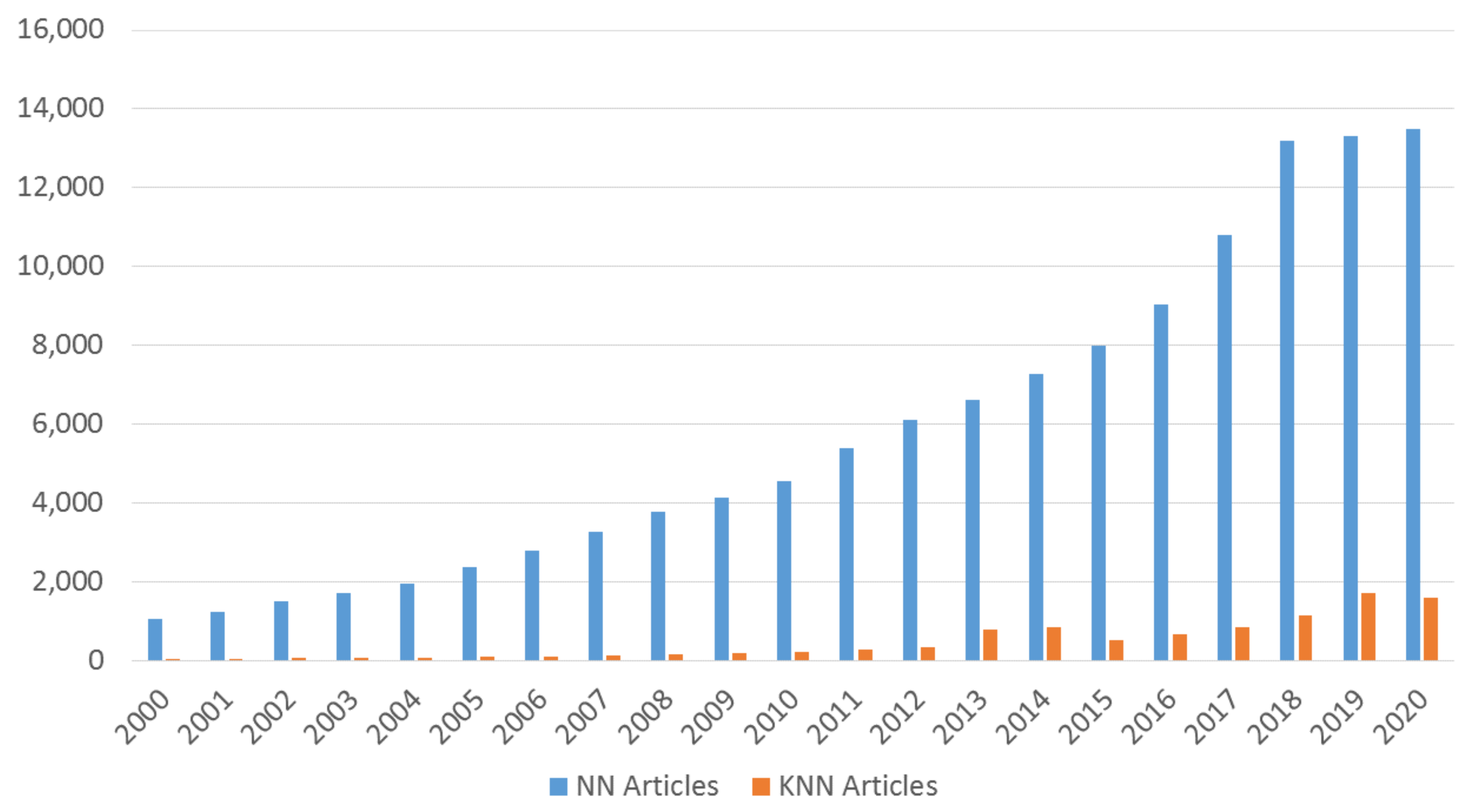
According to the results in regression, DWNN was listed as the top model according to $R^2$ although its performance was very close to that of KNN in the mixed dataset. The result is aligned with the recent literature where DWNN was found superior over other two deep learning methods [62]. Also, it seems a bit surprising that the KNN model was ranked as top 2 for both classification and regression in larger datasets. As a traditional machine learning method, KNN has not drawn as much attention as other trending machine learning methods such as neural networks or deep learning. Figure 11 shows the number of articles as a comparison in terms of the keyword search KNN rainfall forecasting and Neural Network rainfall forecasting respectively in the order of year from Google Scholar. Note that we used the number of publications indexed from Google Scholar as the indicator for the researcher’s interests including peer review sources and non-peer review sources [97] such as thesis, preprint, etc. Our results are also aligned with the recent literature where KNN-based methods were found effective in rainfall forecasting [43,44].

Time series prediction models such as LSTM, GRU, and LSTM-bidirection have not shown satisfactory performance in rainfall forecasting. The overall results showed that LSTM models with relatively short sequence steps (short-term memory) have the better performance than those with longer sequence steps. It might be the very short-term memory characteristics in the short-term hourly rainfall forecasting that affect the performance of the longer sequences. In contrast, the linear based models such as DWNN, linear models, and WNN have much better performance than complicated models such as DNN, SVR, and LSTM. The reason behind the ranking may be that the weather data, unlike other data, contains many uncertain outliers, errors, and missing values that may fuel lots of distractions to the precise models such as neural networks and time series models. Therefore, rainfall forecasting may require more robust models to find the knowledge from those weather datasets. Fortunately, we have found that the SVM and KNN models are qualified for classification and DWNN and KNN are good for regression. However, SVM’s performance in regression was far behind others and DWNN’s performance in classification was not as good as its performance in regression. In contrast, surprisingly, the KNN model that has been long underestimated is robust enough to be qualified for both classification and regression.

Certainly, this study also has some limitations. First, our focus was a generic computing framework that can accommodate a variety of forecasting engines rather than optimizing an individual algorithm inside a specific method. Although the parameters of those bagged machine learning methods have been carefully configured to get the best performance, they are out-of-the-box configurations. Also, limited by the computing resources, our datasets were only from the 11-year weather data in Upstate New York since 2010. Therefore, in the future, we will extend this study on two thrusts: First, refining and enhancing the computing framework to provide more functions such as data preprocessing algorithms [98,99] that can aid to improve the feature selection and reduce the noise to better learn weather features; Second, expanding the datasets with more historically weather data and more regions. We believe that this study and its expansion can advance the method design in this area and benefit the modeling of rainfall forecasting in Upstate New York.

References

1. Reddy, M.J.; Maity, R. Regional rainfall forecasting using large scale climate teleconnections and artificial intelligence techniques. J. Intell. Syst. 2007, 16, 307–322. [Google Scholar]
2. Wu, M.C.; Lin, G.F. The very short-term rainfall forecasting for a mountainous watershed by means of an ensemble numerical weather prediction system in Taiwan. J. Hydrol. 2017, 546, 60–70. [Google Scholar] [CrossRef]
3. Luk, K.C.; Ball, J.; Sharma, A. An application of artificial neural networks for rainfall forecasting. Math. Comput. Model. 2001, 33, 683–693. [Google Scholar] [CrossRef]
4. Thyer, M.; Kuczera, G. A hidden Markov model for modelling long-term persistence in multi-site rainfall time series 1. Model calibration using a Bayesian approach. J. Hydrol. 2003, 275, 12–26. [Google Scholar] [CrossRef]
5. Wang, H.; Asefa, T.; Sarkar, A. A novel non-homogeneous hidden Markov model for simulating and predicting monthly rainfall. Theor. Appl. Climatol. 2021, 143, 627–638. [Google Scholar] [CrossRef]
6. Adamu, L.; Abubakar, U.; Hakimi, D.; Gana, A.S. Prediction of Weekly Rainfall Both in Discrete and Continuous Time Using Markov Model. Int. Res. Environ. Geogr. Earth Sci. 2021, 8, 127–143. [Google Scholar]
7. Cioffi, F.; Conticello, F.; Lall, U.; Marotta, L.; Telesca, V. Large scale climate and rainfall seasonality in a Mediterranean Area: Insights from a non-homogeneous Markov model applied to the Agro-Pontino plain. Hydrol. Process. 2017, 31, 668–686. [Google Scholar]
8. Guo, L.; Jiang, Z.; Chen, W. Using a hidden Markov model to analyze the flood-season rainfall pattern and its temporal variation over East China. J. Meteorol. Res. 2018, 32, 410–420. [Google Scholar] [CrossRef]
9. Stern, R.; Coe, R. A model fitting analysis of daily rainfall data. J. R. Stat. Soc. Ser. 1984, 147, 1–18. [Google Scholar]
10. Lin, G.F.; Chang, M.J.; Huang, Y.C.; Ho, J.Y. Assessment of susceptibility to rainfall-induced landslides using improved self-organizing linear output map, support vector machine, and logistic regression. Eng. Geol. 2017, 224, 62–74. [Google Scholar] [CrossRef]
11. Wu, Y.H.; Nakakita, E. Assessment of landslide hazards using logistic regression with high-resolution radar rainfall observation and geological factor. J. Jpn. Soc. Civ. Eng. Ser. (Hydraul. Eng.) 2019, 75, I_157–I_162. [Google Scholar]
12. Shou, K.J.; Lin, J.F. Evaluation of the extreme rainfall predictions and their impact on landslide susceptibility in a sub-catchment scale. Eng. Geol. 2020, 265, 105434. [Google Scholar] [CrossRef]
13. Hong, H.; Zhu, A. Rainfall induced landslide susceptibility mapping using weight-of-evidence, linear and quadratic discriminant and logistic model tree method. In Proceedings of the AGU Fall Meeting Abstracts, New Orleans, LA, USA, 11–15 December 2017; Volume 2017, p. NH43C-05. [Google Scholar]
14. Hartomo, K.D.; Prasetyo, S.Y.J.; Anwar, M.T.; Purnomo, H.D. Rainfall Prediction Model Using Exponential Smoothing Seasonal Planting Index (ESSPI) For Determination of Crop Planting Pattern. In Computational Intelligence in the Internet of Things; IGI Global: Hershey, PA, USA, 2019; pp. 234–255. [Google Scholar]
15. Dhamodharavadhani, S.; Rathipriya, R. Region-Wise Rainfall Prediction Using MapReduce-Based Exponential Smoothing Techniques. In Advances in Big Data and Cloud Computing; Springer: Singapore, 2019; pp. 229–239. [Google Scholar]
16. Agata, R.; Jaya, I. A comparison of extreme gradient boosting, SARIMA, exponential smoothing, and neural network models for forecasting rainfall data. In Journal of Physics: Conference Series; IOP Publishing: Bristol, UK, 2019; Volume 1397, p. 012073. [Google Scholar]
17. Narayanan, P.; Basistha, A.; Sarkar, S.; Kamna, S. Trend analysis and ARIMA modelling of pre-monsoon rainfall data for western India. Comptes Rendus Geosci. 2013, 345, 22–27. [Google Scholar] [CrossRef]
18. Somvanshi, V.; Pandey, O.; Agrawal, P.; Kalanker, N.; Prakash, M.R.; Chand, R. Modeling and prediction of rainfall using artificial neural network and ARIMA techniques. J. Ind. Geophys. Union 2006, 10, 141–151. [Google Scholar]
19. Eni, D. Seasonal ARIMA modeling and forecasting of rainfall in Warri Town, Nigeria. J. Geosci. Environ. Prot. 2015, 3, 91. [Google Scholar] [CrossRef] [Green Version]
20. Chattopadhyay, S.; Chattopadhyay, G. Univariate modelling of summer-monsoon rainfall time series: Comparison between ARIMA and ARNN. Comptes Rendus Geosci. 2010, 342, 100–107. [Google Scholar] [CrossRef]
21. Swan, T. Generalized Estimating Equations When the Response Variable has a Tweedie Distribution: An Application for Multi-Site Rainfall Modelling. Ph.D. Thesis, University of Southern Queensland, Toowoomba, QLD, Australia, 2006. [Google Scholar]
22. Bahrami, M.; Mahmoudi, M.R. Rainfall modelling using backward generalized estimating equations: A case study for Fasa Plain, Iran. Meteorol. Atmos. Phys. 2020, 132, 771–779. [Google Scholar] [CrossRef]
23. Ingsrisawang, L.; Ingsriswang, S.; Luenam, P.; Trisaranuwatana, P.; Klinpratoom, S.; Aungsuratana, P.; Khantiyanan, W. Applications of statistical methods for rainfall prediction over the Eastern Thailand. In Proceedings of the Multi Conference of Engineers and Computer Scientists, Hong Kong, 17–19 March 2010; pp. 17–19. [Google Scholar]
24. Hacker, K.P.; Sacramento, G.A.; Cruz, J.S.; de Oliveira, D.; Nery, N., Jr.; Lindow, J.C.; Carvalho, M.; Hagan, J.; Diggle, P.J.; Begon, M.; et al. Influence of rainfall on leptospira infection and disease in a tropical urban setting, Brazil. Emerg. Infect. Dis. 2020, 26, 311. [Google Scholar] [CrossRef] [PubMed] [Green Version]
25. Hartini, S.; Hadi, M.P.; Sudibyakto, S.; Poniman, A. Application of Vector Auto Regression Model for Rainfall-River Discharge Analysis. Forum Geogr. 2015, 29. [Google Scholar] [CrossRef] [Green Version]
26. Farook, A.J.; Kannan, K.S. Climate change impact on rice yield in india—Vector autoregression approach. Sri Lankan J. Appl. Stat. 2016, 16. [Google Scholar] [CrossRef]
27. Hong, W.C.; Pai, P.F. Potential assessment of the support vector regression technique in rainfall forecasting. Water Resour. Manag. 2007, 21, 495–513. [Google Scholar] [CrossRef]
28. Lu, W.; Chu, H.; Zhang, Z. Application of generalized regression neural network and support vector regression for monthly rainfall forecasting in western Jilin Province, China. J. Water Supply Res. Technol. 2015, 64, 95–104. [Google Scholar] [CrossRef]
29. Li, G.; Chang, W.; Yang, H. A novel combined prediction model for monthly mean precipitation with error correction strategy. IEEE Access 2020, 8, 141432–141445. [Google Scholar] [CrossRef]
30. Das, D.; Srinivasan, R. Variation of temperature and rainfall in India. Int. J. Adv. Eng. Technol. 2013, 6, 1803. [Google Scholar]
31. Hewage, P.; Trovati, M.; Pereira, E.; Behera, A. Deep learning-based effective fine-grained weather forecasting model. Pattern Anal. Appl. 2021, 24, 343–366. [Google Scholar] [CrossRef]
32. Nayak, D.R.; Mahapatra, A.; Mishra, P. A survey on rainfall prediction using artificial neural network. Int. J. Comput. Appl. 2013, 16, 32–40. [Google Scholar]
33. Darji, M.P.; Dabhi, V.K.; Prajapati, H.B. Rainfall forecasting using neural network: A survey. In Proceedings of the 2015 International Conference on Advances in Computer Engineering and Applications, Ghaziabad, India, 19–20 March 2015; pp. 706–713. [Google Scholar]
34. Nagendra, K.V.; Jahnavi, Y.; Haritha, N. A Survey on Support Vector Machines and Artificial Neural Network in Rainfall Forecasting. Int. J. Future Revolut. Comput. Sci. Commun. Eng. 2017, 3, 20–24. [Google Scholar]
35. Liu, Q.; Zou, Y.; Liu, X.; Linge, N. A survey on rainfall forecasting using artificial neural network. Int. J. Embed. Syst. 2019, 11, 240–249. [Google Scholar] [CrossRef] [Green Version]
36. Salot, N.; Swaminarayan, P.R. A Survey on Rainfall Forecasting using Image Processing Technique. Int. J. Eng. 2015, 3, 126–132. [Google Scholar]
37. Todaro, M. Assessing Irrigation in Western New York State. Master’s Thesis, SUNY College of Environmental Science and Forestry, New York, NY, USA, 2018. [Google Scholar]
38. Wu, J. A Novel Artificial Neural Network Ensemble Model Based on K–Nearest Neighbor Nonparametric Estimation of Regression Function and Its Application for Rainfall Forecasting. In Proceedings of the 2009 International Joint Conference on Computational Sciences and Optimization, Sanya, Hainan, China, 24–26 April 2009; Volume 2, pp. 44–48. [Google Scholar]
39. Liu, S.; Liu, R.; Tan, N. A Spatial Improved-kNN-Based Flood Inundation Risk Framework for Urban Tourism under Two Rainfall Scenarios. Sustainability 2021, 13, 2859. [Google Scholar] [CrossRef]
40. Huang, S.; Huang, M.; Lyu, Y. An Improved KNN-Based Slope Stability Prediction Model. Adv. Civ. Eng. 2020, 2020. [Google Scholar] [CrossRef]
41. Ahmed, K.; Sachindra, D.; Shahid, S.; Iqbal, Z.; Nawaz, N.; Khan, N. Multi-model ensemble predictions of precipitation and temperature using machine learning algorithms. Atmos. Res. 2020, 236, 104806. [Google Scholar] [CrossRef]
42. Jan, Z.; Abrar, M.; Bashir, S.; Mirza, A.M. Seasonal to inter-annual climate prediction using data mining KNN technique. In Proceedings of the International Multi Topic Conference, Karachi, Pakistan, 23–24 December 2008; pp. 40–51. [Google Scholar]
43. Huang, M.; Lin, R.; Huang, S.; Xing, T. A novel approach for precipitation forecast via improved K-nearest neighbor algorithm. Adv. Eng. Inform. 2017, 33, 89–95. [Google Scholar] [CrossRef]
44. Yang, M.; Wang, H.; Jiang, Y.; Lu, X.; Xu, Z.; Sun, G. Geca proposed ensemble–knn method for improved monthly runoff forecasting. Water Resour. Manag. 2020, 34, 849–863. [Google Scholar] [CrossRef]
45. Hu, J.; Liu, J.; Liu, Y.; Gao, C. EMD-KNN model for annual average rainfall forecasting. J. Hydrol. Eng. 2013, 18, 1450–1457. [Google Scholar] [CrossRef]
46. Mehdizadeh, S. Using AR, MA, and ARMA time series models to improve the performance of MARS and KNN approaches in monthly precipitation modeling under limited climatic data. Water Resour. Manag. 2020, 34, 263–282. [Google Scholar] [CrossRef]
47. Hasan, N.; Nath, N.C.; Rasel, R.I. A support vector regression model for forecasting rainfall. In Proceedings of the 2015 2nd International Conference on Electrical Information and Communication Technologies (EICT), Dhaka, Bangladesh, 21–23 May 2015; pp. 554–559. [Google Scholar]
48. Bojang, P.O.; Yang, T.C.; Pham, Q.B.; Yu, P.S. Linking singular spectrum analysis and machine learning for monthly rainfall forecasting. Appl. Sci. 2020, 10, 3224. [Google Scholar] [CrossRef]
49. Yu, P.S.; Yang, T.C.; Chen, S.Y.; Kuo, C.M.; Tseng, H.W. Comparison of random forests and support vector machine for real-time radar-derived rainfall forecasting. J. Hydrol. 2017, 552, 92–104. [Google Scholar] [CrossRef]
50. Tao, H.; Sulaiman, S.O.; Yaseen, Z.M.; Asadi, H.; Meshram, S.G.; Ghorbani, M. What is the potential of integrating phase space reconstruction with SVM-FFA data-intelligence model? Application of rainfall forecasting over regional scale. Water Resour. Manag. 2018, 32, 3935–3959. [Google Scholar] [CrossRef]
51. French, M.N.; Krajewski, W.F.; Cuykendall, R.R. Rainfall forecasting in space and time using a neural network. J. Hydrol. 1992, 137, 1–31. [Google Scholar] [CrossRef]
52. Koizumi, K. An Objective Method to Modify Numerical Model Forecasts with Newly Given Weather Data Using an Artificial Neural Network. Weather. Forecast. 1999, 14, 109–118. [Google Scholar] [CrossRef]
53. Toth, E.; Brath, A.; Montanari, A. Comparison of short-term rainfall prediction models for real-time flood forecasting. J. Hydrol. 2000, 239, 132–147. [Google Scholar] [CrossRef]
54. Sulaiman, J.; Wahab, S.H. Heavy rainfall forecasting model using artificial neural network for flood prone area. In IT Convergence and Security 2017; Springer: Singapore, 2018; pp. 68–76. [Google Scholar]
55. Canchala, T.; Alfonso-Morales, W.; Carvajal-Escobar, Y.; Cerón, W.L.; Caicedo-Bravo, E. Monthly rainfall anomalies forecasting for southwestern Colombia using artificial neural networks approaches. Water 2020, 12, 2628. [Google Scholar] [CrossRef]
56. Hossain, I.; Rasel, H.; Imteaz, M.A.; Mekanik, F. Long-term seasonal rainfall forecasting using linear and non-linear modelling approaches: A case study for Western Australia. Meteorol. Atmos. Phys. 2020, 132, 131–141. [Google Scholar] [CrossRef]
57. Yaseen, Z.M.; Ghareb, M.I.; Ebtehaj, I.; Bonakdari, H.; Siddique, R.; Heddam, S.; Yusif, A.A.; Deo, R. Rainfall pattern forecasting using novel hybrid intelligent model based ANFIS-FFA. Water Resour. Manag. 2018, 32, 105–122. [Google Scholar] [CrossRef]
58. Jaddi, N.S.; Abdullah, S. Optimization of neural network using kidney-inspired algorithm with control of filtration rate and chaotic map for real-world rainfall forecasting. Eng. Appl. Artif. Intell. 2018, 67, 246–259. [Google Scholar] [CrossRef]
59. Hung, N.Q.; Babel, M.S.; Weesakul, S.; Tripathi, N. An artificial neural network model for rainfall forecasting in Bangkok, Thailand. Hydrol. Earth Syst. Sci. 2009, 13, 1413–1425. [Google Scholar] [CrossRef] [Green Version]
60. Cheng, H.T.; Koc, L.; Harmsen, J.; Shaked, T.; Chandra, T.; Aradhye, H.; Anderson, G.; Corrado, G.; Chai, W.; Ispir, M.; et al. Wide & deep learning for recommender systems. In Proceedings of the 1st Workshop on Deep Learning for Recommender Systems, Boston, MA, USA, 15 September 2016; pp. 7–10. [Google Scholar]
61. Pölsterl, S.; Sarasua, I.; Gutiérrez-Becker, B.; Wachinger, C. A wide and deep neural network for survival analysis from anatomical shape and tabular clinical data. In Proceedings of the Joint European Conference on Machine Learning and Knowledge Discovery in Databases, Würzburg, Germany, 16–20 September 2019; pp. 453–464. [Google Scholar]
62. Bajpai, V.; Bansal, A. A Deep and Wide Neural Network-based Model for Rajasthan Summer Monsoon Rainfall (RSMR) Prediction. arXiv 2021, arXiv:2103.02157. [Google Scholar]
63. Coble, N.J.; Yu, N. A Reservoir Computing Scheme for Multi-class Classification. In Proceedings of the 2020 ACM Southeast Conference, Tampa, FL, USA, 2–4 April 2020; pp. 87–93. [Google Scholar]
64. Gallicchio, C.; Micheli, A. Deep echo state network (deepesn): A brief survey. arXiv 2017, arXiv:1712.04323. [Google Scholar]
65. Yen, M.H.; Liu, D.W.; Hsin, Y.C.; Lin, C.E.; Chen, C.C. Application of the deep learning for the prediction of rainfall in Southern Taiwan. Sci. Rep. 2019, 9, 1–9. [Google Scholar] [CrossRef] [Green Version]
66. Vlachas, P.R.; Pathak, J.; Hunt, B.R.; Sapsis, T.P.; Girvan, M.; Ott, E.; Koumoutsakos, P. Backpropagation algorithms and reservoir computing in recurrent neural networks for the forecasting of complex spatiotemporal dynamics. Neural Netw. 2020, 126, 191–217. [Google Scholar] [CrossRef] [Green Version]
67. Ouyang, Q.; Lu, W. Monthly rainfall forecasting using echo state networks coupled with data preprocessing methods. Water Resour. Manag. 2018, 32, 659–674. [Google Scholar] [CrossRef]
68. Coulibaly, P. Reservoir computing approach to Great Lakes water level forecasting. J. Hydrol. 2010, 381, 76–88. [Google Scholar] [CrossRef]
69. De Vos, N. Reservoir computing as an alternative to traditional artificial neural networks in rainfall-runoff modelling. Hydrol. Earth Syst. Sci. Discuss. 2012, 9, 6101–6134. [Google Scholar]
70. Bezerra, S.G.; de Andrade, C.B.; Valença, M.J. Using reservoir computing and trend information for short-term streamflow forecasting. In Proceedings of the International Conference on Artificial Neural Networks, Barcelona, Spain, 6–9 September 2016; pp. 308–316. [Google Scholar]
71. Liu, M.; Huang, Y.; Li, Z.; Tong, B.; Liu, Z.; Sun, M.; Jiang, F.; Zhang, H. The applicability of LSTM-KNN model for real-time flood forecasting in different climate zones in China. Water 2020, 12, 440. [Google Scholar] [CrossRef] [Green Version]
72. Chhetri, M.; Kumar, S.; Pratim Roy, P.; Kim, B.G. Deep BLSTM-GRU Model for Monthly Rainfall Prediction: A Case Study of Simtokha, Bhutan. Remote Sens. 2020, 12, 3174. [Google Scholar] [CrossRef]
73. Hernández, E.; Sanchez-Anguix, V.; Julian, V.; Palanca, J.; Duque, N. Rainfall prediction: A deep learning approach. In Proceedings of the International Conference on Hybrid Artificial Intelligence Systems, Seville, Spain, 18–20 April 2016; pp. 151–162. [Google Scholar]
74. Salman, A.G.; Kanigoro, B.; Heryadi, Y. Weather forecasting using deep learning techniques. In Proceedings of the 2015 International Conference on Advanced Computer Science and Information Systems (ICACSIS), Depok, Indonesia, 10–11 October 2015; pp. 281–285. [Google Scholar]
75. Hu, C.; Wu, Q.; Li, H.; Jian, S.; Li, N.; Lou, Z. Deep learning with a long short-term memory networks approach for rainfall-runoff simulation. Water 2018, 10, 1543. [Google Scholar] [CrossRef] [Green Version]
76. Klemmer, K.; Saha, S.; Kahl, M.; Xu, T.; Zhu, X.X. Generative modeling of spatio-temporal weather patterns with extreme event conditioning. arXiv 2021, arXiv:2104.12469. [Google Scholar]
77. Hossain, M.; Rekabdar, B.; Louis, S.J.; Dascalu, S. Forecasting the weather of Nevada: A deep learning approach. In Proceedings of the 2015 International Joint Conference on Neural Networks (IJCNN), Killarney, Ireland, 11–16 July 2015; pp. 1–6. [Google Scholar] [CrossRef]
78. Karevan, Z.; Suykens, J.A. Spatio-temporal stacked LSTM for temperature prediction in weather forecasting. arXiv 2018, arXiv:1811.06341. [Google Scholar]
79. Mittal, S.; Sangwan, O.P. Big Data Analytics Using Deep LSTM Networks: A Case Study for Weather Prediction. Adv. Sci. Technol. Eng. Syst. J. 2020, 5, 133–137. [Google Scholar] [CrossRef] [Green Version]
80. Qiu, M.; Zhao, P.; Zhang, K.; Huang, J.; Shi, X.; Wang, X.; Chu, W. A Short-Term Rainfall Prediction Model Using Multi-task Convolutional Neural Networks. In Proceedings of the 2017 IEEE International Conference on Data Mining (ICDM), New Orleans, LA, USA, 18–21 November 2017; pp. 395–404. [Google Scholar] [CrossRef]
81. Yu, N.; Li, Z.; Yu, Z. Survey on encoding schemes for genomic data representation and feature learning—From signal processing to machine learning. Big Data Min. Anal. 2018, 1, 191–210. [Google Scholar]
82. Ioffe, S.; Szegedy, C. Batch normalization: Accelerating deep network training by reducing internal covariate shift. In Proceedings of the International Conference on Machine Learning, Lille, France, 6–11 July 2015; pp. 448–456. [Google Scholar]
83. Bjorck, J.; Gomes, C.; Selman, B.; Weinberger, K.Q. Understanding batch normalization. arXiv 2018, arXiv:1806.02375. [Google Scholar]
84. Zhang, H.; Dauphin, Y.N.; Ma, T. Fixup initialization: Residual learning without normalization. arXiv 2019, arXiv:1901.09321. [Google Scholar]
85. Luo, P.; Ren, J.; Peng, Z.; Zhang, R.; Li, J. Differentiable learning-to-normalize via switchable normalization. arXiv 2018, arXiv:1806.10779. [Google Scholar]
86. Basodi, S.; Baykal, P.I.; Zelikovsky, A.; Skums, P.; Pan, Y. Analysis of heterogeneous genomic samples using image normalization and machine learning. BMC Genom. 2020, 21, 1–10. [Google Scholar] [CrossRef] [PubMed]
87. Park, T.; Liu, M.Y.; Wang, T.C.; Zhu, J.Y. Semantic image synthesis with spatially-adaptive normalization. In Proceedings of the IEEE/CVF Conference on Computer Vision and Pattern Recognition, Long Beach, CA, USA, 16–20 June 2019; pp. 2337–2346. [Google Scholar]
88. Cooijmans, T.; Ballas, N.; Laurent, C.; Gülçehre, Ç.; Courville, A. Recurrent batch normalization. arXiv 2016, arXiv:1603.09025. [Google Scholar]
89. Wu, Y.; He, K. Group normalization. In Proceedings of the European Conference on Computer Vision (ECCV), Munich, Germany, 8–14 September 2018; pp. 3–19. [Google Scholar]
90. Santurkar, S.; Tsipras, D.; Ilyas, A.; Madry, A. How does batch normalization help optimization? arXiv 2018, arXiv:1805.11604. [Google Scholar]
91. Singh, D.; Singh, B. Investigating the impact of data normalization on classification performance. Appl. Soft Comput. 2020, 97, 105524. [Google Scholar] [CrossRef]
92. Jo, J.M. Effectiveness of normalization pre-processing of big data to the machine learning performance. J. Korea Inst. Electron. Commun. Sci. 2019, 14, 547–552. [Google Scholar]
93. National Oceanic and Atmospheric Administration, Department of Defense, Federal Aviation Administration, and United States Navy. Automated Surface Observing System (ASOS) User’s Guide; National Oceanic and Atmospheric Administration: Washington, DC, USA, 1998. [Google Scholar]
94. Cherkassky, V.; Ma, Y. Practical selection of SVM parameters and noise estimation for SVM regression. Neural Netw. 2004, 17, 113–126. [Google Scholar] [CrossRef] [Green Version]
95. Hochreiter, S.; Schmidhuber, J. Long short-term memory. Neural Comput. 1997, 9, 1735–1780. [Google Scholar] [CrossRef] [PubMed]
96. Cho, K.; Van Merriënboer, B.; Gulcehre, C.; Bahdanau, D.; Bougares, F.; Schwenk, H.; Bengio, Y. Learning phrase representations using RNN encoder-decoder for statistical machine translation. arXiv 2014, arXiv:1406.1078. [Google Scholar]
97. Martín-Martín, A.; Orduna-Malea, E.; Thelwall, M.; López-Cózar, E.D. Google Scholar, Web of Science, and Scopus: A systematic comparison of citations in 252 subject categories. J. Inf. 2018, 12, 1160–1177. [Google Scholar] [CrossRef] [Green Version]
98. Unnikrishnan, P.; Jothiprakash, V. Daily rainfall forecasting for one year in a single run using Singular Spectrum Analysis. J. Hydrol. 2018, 561, 609–621. [Google Scholar] [CrossRef]
99. Haidar, A.; Verma, B. A novel approach for optimizing climate features and network parameters in rainfall forecasting. Soft Comput. 2018, 22, 8119–8130. [Google Scholar] [CrossRef]
Figure 1. Weather stations in Upstate New York. The blue circle indicates that ROC dataset is from Rochester station and the red circles are Buffalo’s two stations, Syracuse’s two stations, and Albany’s two stations. Both the blue and red circles contribute to the mixed dataset.
Informatics 08 00047 g001
Figure 2. The illustration of a generic computing framework for regional rainfall forecasting.
Informatics 08 00047 g002
Figure 3. The feature matrix in ROC dataset. Notation: tmpf, air temperature in Fahrenheit typically at 2 m; dwpf, dew point temperature in Fahrenheit typically at 2 m; relh, relative humidity in %; drct, wind direction in degrees from north; sknt, wind speed in knots; alti, pressure altimeter in inches; mslp, sea level pressure in millibar; vsby, visibility in miles.
Informatics 08 00047 g003
Figure 4. An illustration of perceptron structure.
Informatics 08 00047 g004
Figure 5. An illustration of DWNN.
Informatics 08 00047 g005
Figure 6. An illustration of reservoir computing [63].
Informatics 08 00047 g006
Figure 7. An illustration of LSTM structure.
Informatics 08 00047 g007
Figure 8. The illustration of confusion matrix.
Informatics 08 00047 g008
Figure 9. Classification performance. (AC): Classification ranking in the Mixed dataset. (DF): Classification ranking in the ROC dataset. (A,D): The best performance ranking mixing the normalization. (B,E): Accuracy in regard to normalization. (C,F): An overall ranking among models and normalizations.
Informatics 08 00047 g009
Figure 10. Running time for training and inference.
Informatics 08 00047 g010
Figure 11. The number of indexed articles for KNN and Neural Network used in rainfall forecasting from Google Scholar as of 20 Junuary 2021.
Informatics 08 00047 g011