Article

The Effect of Object Geometric Features on Frequency Inflection Point of Underwater Active Electrolocation System

School of Automation Engineering, University of Electronic Science and Technology of China, Chengdu 610054, China
*
Author to whom correspondence should be addressed.
J. Mar. Sci. Eng. 2021, 9(7), 756; https://doi.org/10.3390/jmse9070756
Submission received: 11 June 2021 / Revised: 2 July 2021 / Accepted: 4 July 2021 / Published: 8 July 2021
(This article belongs to the Section Ocean Engineering)

Abstract

:
Biologists have discovered a kind of weakly electric fish that identifies its prey by using active electrolocation in virtual darkness. In this study, we built an underwater active electrolocation system platform designed to investigate the biological mechanism allowing these fish to distinguish objects and determine how the amplitude information-frequency characteristic (AIFC) response are affected by the geometric characteristics of target objects in the active electrolocation system. We used a single-frequency sinusoidal signal to scan metal objects in different orientations and observed the amplitude information response variation of the disturbed detection signal. The detection frequency dead zone (DFDZ) and the frequency inflection point (FIP) were used to characterize the variation. In addition, we repeated the experiments after replacing the metal objects with objects of different materials and geometric characteristics to summarize the general laws. Our results showed that the FIP value of the detection signal was lowest when the object was detected in the orientation of its corner and highest when the object was detected in the orientation of its surface. The geometrical characteristics of metal objects in different orientations have a certain influence on the amplitude of the detection signal. Article Highlights: (1) The general law between the shape of metal probed objects, and electric field detection signal was found and summarized. (2) We used a single-frequency sinusoidal signal to scan regular metal probed objects, and it was found that the frequency inflection point (FIP) of the metal probed objects edge was the highest, whereas that of the corner was the lowest. (3) The shape of a metal object can be recognized by scanning regular metal objects with an electric field signal.

1. Introduction

Many aquatic creatures, such as sharks, sturgeons, catfish, and other fish, can perceive electric field information around them and determine the locations of the sources of electric fields, which is called passive electrolocation [1,2]. Other fish, however, use active electrolocation systems, meaning they actively emit electrical signals into the environment and perceive these signals after they have been disturbed by the external world [3]. Weakly electric fish, such as Peters’ elephantnose fish (Gnathonemus petersii), can emit weak electric signals into the environment through electroreceptor organs. The electric field signal is distorted when it approaches surrounding objects. Weakly electric fish perceive these weak signals through their epidermal electroreceptor organs thus as to generate an ‘electric image’ (the pattern of voltage change). Analysis of the ‘electric image’ enables the fish to measure the distance, three-dimensional shape, and other attributes of surrounding objects [3,4,5,6]. Weakly electric fish can identify prey and communicate by perceiving these signals. In 1996, Rasnow found that weakly electric fish’s electroreceptor organs are distributed in the skin, and the tissues that emit electric signals are distributed in the tail. Electric images produced on the fish’s epidermis change with the surrounding electric field [7]. In 1998, Caputi et al. found that the change of electric field information of weakly electric fish is related to the conductivity of the medium and objects in the surrounding environment. In the same year, Nelson et al. and MacIver et al. demonstrated that the change is also related to the electrical characteristics of objects and the distance between objects and weakly electric fish [8,9,10]. In 2003, the influence of several objects on the active electrolocation system of weakly electric fish was studied by Adriana Migliaro et al. The results demonstrated that the electric field information was not a simple linear overlay of each object, but the electric fields affected each other when multiple objects surrounded the fish [11]. In fact, there are many factors that affect the electrical image: the volume of the object, some physical and chemical characteristics of the object, the distance of the object from the weakly electric fish, the conductivity of the object, and the conductivity of the medium environment [5,12,13]. In 2003, Lebastard et al. practically applied it to underwater active electrolocation and tried to measure the size of the object [14]. In 2004, active electric field technology was applied to underwater vehicles for the first time, and its rationality was validated [10,15]. In 2008, Solberg et al. began to apply it to the positioning of underwater objects [16]. In 2012, Noël Servagent et al. developed a sensor model based on underwater active electrolocation [17]. In 2015, Dimble et al. proposed and experimentally verified an obstacle avoidance strategy based on active electric field detection [18]. In 2016, Bai et al. determined an algorithm that could estimate the size, distance, and shape of prolate spheroids, and they employed an active motion and supervised learning approach that estimates object shape in a sequential manner with a reasonable level of accuracy [19]. In 2019, Fujita et al. used different shapes of resistive objects and demonstrated that an integration effect of the peak amplitude and half-maximum width could be an invariant measure of object shape [20]. Gottwald et al. designed an electric camera device that probed underwater objects with a weak electric field and captured ‘electric images’ of the targets [21].
Active electrolocation system theories have been developed for many years. In 2015, Peng studied the amplitude-frequency response of varying sinusoidal electric field frequencies to the probed object of underwater active electrolocation systems and proposed the detect frequency dead zone (DFDZ) and frequency inflection point (FIP) of amplitude information-frequency characteristics (AIFC) [22]. Peng’s AIFC study played a significant role in researching the relationship between an object’s features and the active electrolocation system. By comparing the FIPs of probed objects made of three different materials and in two different shapes, Peng et al. found that the shape of the probed object had a significant effect on the FIP of the AIFC for the electrolocation system [23]. Peng also established a mathematical model based on the Cole–Cole model (CCM), which explained why DFDZ and FIP exist in electrolocation systems [22]. However, Peng did not research the details of the relationship between the AIFC and the geometric properties of probed objects. Thus, additional work needs to be conducted. In 2019, Ren et al. studied the AIFC for multi-frequency excitation of underwater active electrolocation systems, finding that graphite electrodes performed much better than titanium electrodes for multi-frequency signal detection [24]. Besides, they employed multi-frequency signals for excitation and gained the FIP of underwater objects efficiently and accurately on the basis of Peng’s work. However, Ren et al. did not study clear correlations between multi-frequency signals and the shapes of objects. In 2020, Bazeille et al. [25] proposed a new model-based heuristic method for an active electrolocation system, which realized the parallel measurement of object location and size. The method is a purely model-based method, using a new dedicated score function as a comparison criterion to select the model that best fits with the object among a pool of possible models. However, the score function is weakly sensitive to the angle between the object and the sensor. When the angle is close to 90°, the size error is larger. Moreover, this method fails to measure the shape of the object. Therefore, we can study the relationship between AIFC and the shape of the object and whether the relationship can be used to measure the shape of the object, thus as to avoid the influence of angle in the new model-based heuristic method.
In this paper, we investigated how the FIP of AIFC is affected by the shape of the probed object in an active electrolocation system. Inspired by the active electrolocation mechanism of weakly electric fish, we developed a bionic experimental platform. We assumed that the shapes of objects in different orientations exposed to the active electric field would affect the FIP value. Owing to the limitations of the experimental platform, we changed the shape of the objects exposed to the electric field by rotating them. Multiple FIPs were measured for fixed angles made by the orientations of the probed objects. Peng found that FIP does not exist for polymer insulating material objects [22], thus in our experiments, we used metal conductors as the probed objects. Specifically, aluminum, copper and steel were selected. Then, in order to determine clear correlations between FIP and object shape, we tested the following regular geometric objects: quadrangular prism, hexagonal prism, octagonal prism, cylinder, quadrangular pyramid, hexagonal pyramid, octagonal pyramid, cone, and triangular pyramid. When the angle between the probed object and the electric field was changed by rotating the object, we measure the DFDZ and FIP of the AIFC of the object. Then we compared the FIPs of the differently shaped objects at different rotation angles to find the general law of changes. Furthermore, we demonstrated that the FIP of a metal probed object is directly related to the shape of the object.

2. Materials and Methods

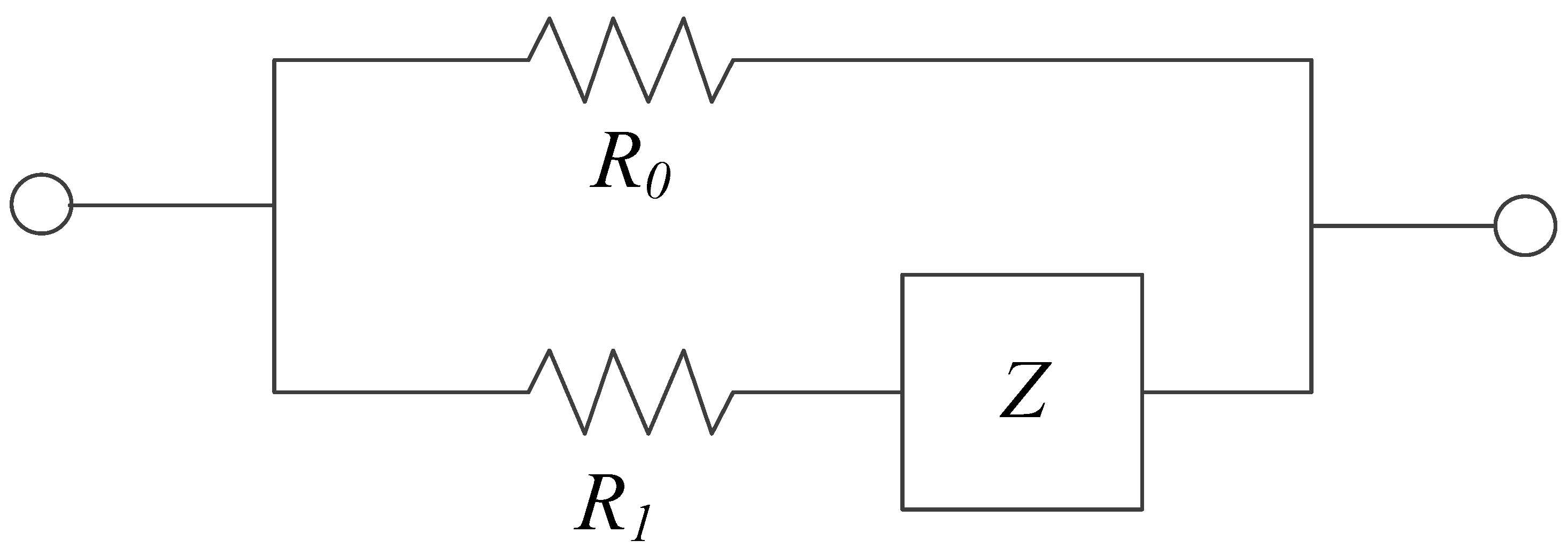
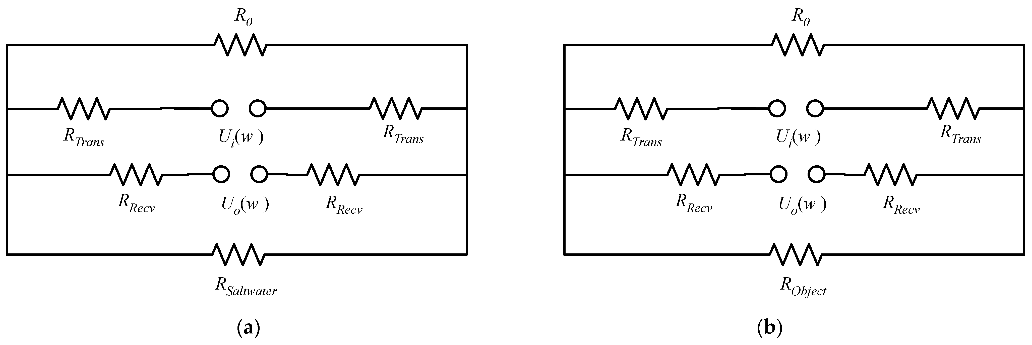
2.1. Theoretical Analysis

A weakly electric fish has an electric organ (EO) at the base of its tail, which can emit electrical signals, called electric organ discharge (EOD), to the surroundings. When there is a conductive object around a weakly electric fish, the amplitude and phase of the fish’s EOD will change [26]. DFDZ and FIP phenomena cannot be explained by electromagnetic field theory because the frequency-dependent behavior of electrical conductivity shows when conductors are present in the underwater electric field. This is called the induced polarization (IP) effect.
As Figure 1 depicts, the Cole–Cole model introduced in 1941 [27] was built based on object resistance R1 in series with complex impedance Z, which both were parallel with water medium resistance R0. In this model, Z = ( i ω X ) c is the equivalent resistance for the IP effect of objects.
In Figure 1, ω is the angular frequency of a sinusoidal electric excitation (ω = 2πf), f is the frequency, and X = τ ( R 0 m ) 1 c , where m is the chargeability and τ is the time constant. In general, 0 < c < 1, and the typical value of c is 0.25. When f → 0, |Z| → ∞, and when f → ∞, |Z| → 0. The model indicates that Z is related only to the electrical characteristics of the probed objects and the surrounding environment. Based on this premise, an equivalent circuit model of the underwater active electrolocation system (UAES) was established, as shown in Figure 2. A total of 2 emitter electrodes were used as dipole emitters, and 2 receiver electrodes were used to measure the voltage difference at that point. To obtain more information, the receiving electrodes and the transmitting electrodes adopted an asymmetric structure.
Parallel conduction through a purely resistive element is simulated by the resistance R0, RTrans(ω) is the equivalent impedance of the transmitting electrode, and RRecv(ω) is the equivalent impedance of the receiving electrode. When there is no object in the water (Figure 2a), the measured voltage is expressed as UObject. When the probed object is directly below the detection electrodes (Figure 2b), RObject(ω) is the equivalent impedance of the probed object and its IP effect. RSaltwater is the equivalent impedance of the water that is drained by the probed object. The measured voltage is expressed as Ufree.
If the equivalent impedance of the measured area is greater than the impedance of the same volume of water, ΔU = UObject − Ufree > 0. Thus, when the electrode scans the probed object, the AIFC exhibits a convex shape, defined as the positive characteristic. If the equivalent impedance of the measured area is smaller than the impedance of the same volume of water, ΔU < 0 and the AIFC exhibits a concave shape, defined as the negative characteristic. Specifically, when the probed object has an IP effect, its AIFC will exhibit positive characteristics for lower frequency excitation and negative characteristics for higher frequency excitation. At a particular frequency in between, the AIFC will exhibit neither positive nor negative characteristics. This frequency inflection point (FIP) is denoted as fFIP. When the frequency of excitation is near the FIP, we cannot detect the characteristics of the probed object. This frequency range is defined as the DFDZ [22].

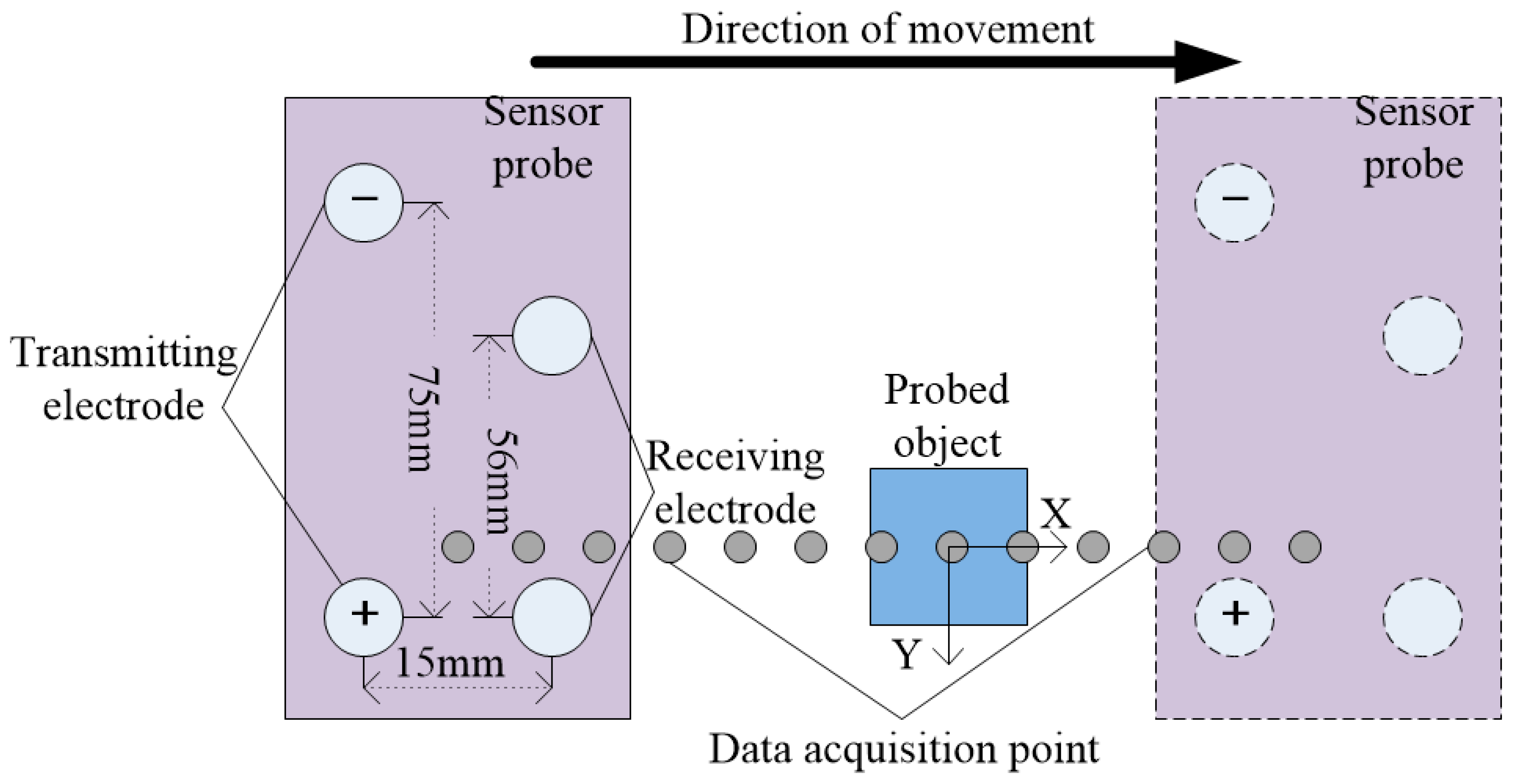
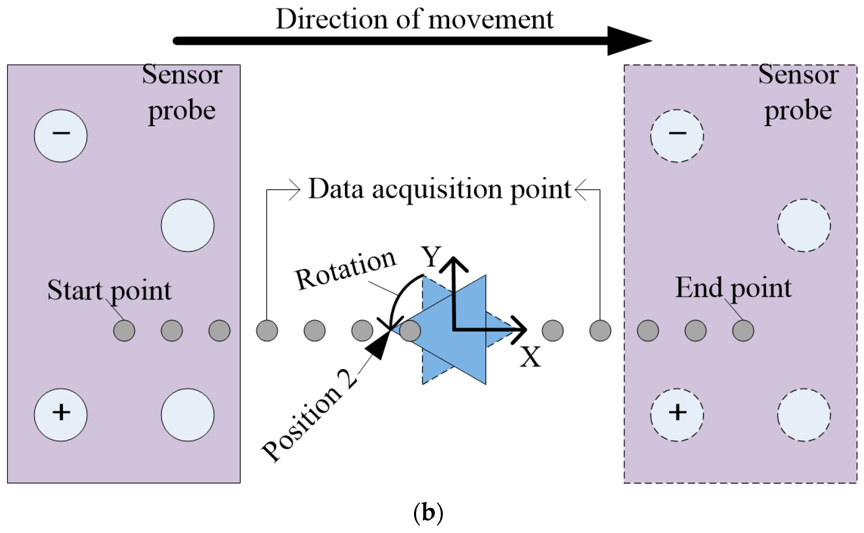
2.2. Experiment Setup

Based on the principle of active electrolocation of weakly electric fish, we built an underwater active electric field experimental platform as shown in Figure 3. The platform mainly included 4parts: an experiment detected environment, a sensor probe module, a motion module, and a data processing module. In Figure 3, ① represents the data acquisition board, ② represents the electrode holder, ③ represents the electrode, ④ represents the triaxial motor controller, ⑤ represents the probed object, ⑥ represents the PC.
To facilitate observation and reduce external interference, we used a plexiglass tank with a size of 90 cm × 57 cm × 40 cm as the water environment container for the experiment. Tap water was selected as the experimental water environment, and an appropriate amount of sodium chloride was added to adjust the conductivity of the water. The sensor probe module was used to simulate the swimming function of weakly electric fish in the detected environment. The sensor probe module mainly consisted of an external electrode terminal, reserved electrode mounting hole, electrode bracket, signal transmitting electrode, and signal receiving electrode. The transmitting electrode was used to establish the underwater active detection electric field, and the receiving electrode was used to collect the disturbed electric field signal. The distance between 2 transmitting electrodes was 7.5 cm, and the distance between 2 receiving electrodes was 5.6 cm. The 4 electrodes were all made of titanium alloy with a resistivity of 1.75 × 10⁻⁸ Ω·m. To simplify the experiment, the motion module controlled the sensor probe to move from left to right along the X-axis. The movement speed was set to 3 mms−1 to ensure adequate sampling points were obtained for each waveform. A schematic of the experimental setup is shown in Figure 4. In this experiment, we used the signal generator HDG2102B as the signal source of the transmitting electrode, and an NI USB-6289 data acquisition (DAQ) board was used to collect data from the receiving electrodes. The collected data were analyzed and processed by professional data processing software DIAdem and Origin.

2.3. Data Processing
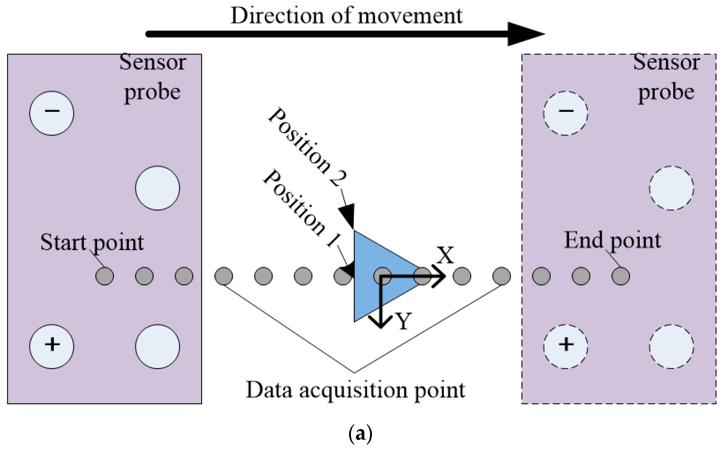
In the experiment, the amplitude of the active electric field changed very weakly and was susceptible to external interference. Therefore, the frequency components in the collected data changed with time. To observe the change of signal frequency and amplitude with time, the short-time Fourier transform (STFT) was used to analyze the experimental data.
STFT uses the sliding time window function to divide the signal into many small signal segments, which are regarded as linear stationary signals. The Fourier transform is then applied to the small segments of the signal, and the center point of each small segment of the signal is used as a time index to indicate the time point of the signal frequency. When the signal is a continuous function, x(t) represents the continuous signal function and ω(t) represents the window function. Then the expression of STFT can be expressed as follows Equation (1):
STFT ( t , Ω ) = x ( t + τ ) ω ( τ ) e j Ω t d τ
In the experiment, the electric field received signal was a discrete signal after passing through the data acquisition card, thus we needed to use the discrete STFT to process the data. We used Δt to represent the sampling time interval, and we made the following substitutions: x(n) = x(mΔt) Δt, ω = ΩΔt. Then the discrete STFT expression could be obtained, as shown in the following Equation (2):
STFT ( n , ω ) = m = x ( n + m ) ω ( m ) e j m ω Δ t
where ω(m) is the window function, and m and n are integers (0, 1, 2, 3…). When n takes a different value, the window moves along x, and ω(m) is a sliding window. The STFT cyclically changes with ω(m), with a period of 2n.
In the experiment, the Hanning window was used as the window function. By continuously sliding the time window function and calculating the signal segments intercepted by the window function, a 3-dimensional spectrogram, namely, the joint time-frequency spectrogram (JTFS), can be obtained, from which the change of signal frequency with time can be observed, and the DFDZ and FIP of the detected object can be found.

2.4. Procedures

This study focused on the influence of geometric features of target objects in different orientations on an active electric field, thus it was necessary to detect and collect distorted electric field information of target objects in different orientations. As shown in Figure 4, without affecting the experimental results, we reduced the amount of data by collecting discrete point data in different orientations. In the figure, each point represents the electric field information collected at the current position, and the square represents the detected object. During the experiment, the sensor probe needed to be immersed in water and moved over the detected target object at a uniform speed. Then the AIFC of the distorted electric field collected in each experiment was transformed into the frequency domain for analysis and processing. The sensor probe swept the frequency in a certain orientation of the current target object. After collecting a set of data, it was necessary to rotate the sensor probe by an angle with the target object as the center point thus as to ensure that the collected information was the interference of the geometric features of the target object in different orientations on the detection signal.

2.5. The DFDZ of Objects

As shown in Figure 5a, the blue part was the detected object, that was, the copper triangular pyramid, with a bottom edge length of 11.2 mm and a height of 40 mm. The sensor probe moved at a constant speed along the fixed track and collected data once at every fixed distance.
According to the relative motion diagram shown in Figure 5a, we used a sinusoidal excitation signal with an amplitude of 2 V and a frequency of 30 Hz to scan each probed object. The discrete STFT was applied to the data collected by the receiving electrode to obtain the joint time-frequency spectrogram, as shown in Figure 6a. The X-axis represents the frequency distribution of the received signal (Hz), the Y-axis represents the time of the detection device during operation (s), and the Z-axis represents the peak amplitude of the signal after the Fourier transform (V). After observing the spectrum, we found that the signal amplitude showed an “upward convex” change trend with time. Then, the frequency was set to 40 Hz, 50 Hz, and 60 Hz, and the method mentioned above was repeated. The spectrum obtained is shown in Figure 6.
By comparing the amplitude variation trend of the detected object spectrum at 4 groups of different frequencies in Figure 6, we found that the amplitude curve of the detected object gradually changed from convex to concave with the increase of excitation signal frequency. We referred to this phenomenon as the phenomenon of DFDZ and FIP [22]. The critical frequency point at which the amplitude curve changed from convex to concave was called the FIP. From Figure 6, we concluded that the DFDZ of the probed objects was 50–60 Hz, thus we took 55 Hz as the FIP. Next, we experimented 3 times to verify whether the FIP and DFDZ of the copper triangular pyramid will fluctuate in this orientation. Repeat 3 sets of the same experiment, and the final experiment shows that both DFDZ and FIP were consistent, that was, the standard deviation of DFDZ and FIP was 0. In order to simplify the subsequent experimental steps, the following experiments were conducted only once in the same orientation.

3. Results

To study the relationship between object shape and underwater active electrolocation, we scanned and detected two orientations of a copper triangular pyramid and found that the DFDZ values of the two orientations were different. Then, we replaced the triangular pyramid with a cone and conducted the experiment as a control group according to the method mentioned above. The experimental results proved that the difference between the two orientations of DFDZ was caused by the different surface features of the object in different orientations. Then, we selected the copper quadrangular prism as the experimental object, added an orientation to scan and detect the detected object, analyzed the experimental results, and summarized the general law between the surface characteristics of the object and its DFDZ. Finally, we chose different geometries of iron and aluminum as experimental objects to generalize the generality of the above laws and focused on studying the relationship between object shape and the underwater active detection electric field system, looking for the correlation between object shape and FIP and summarizing the general laws.

3.1. The Relationship between Surface Characteristics and FIP

We found that the FIP of one orientation of the triangular pyramid was 45 Hz. The next step was to detect the second orientation of the triangular pyramid. Since the detection device of the experimental platform cannot realize 360° rotation, we could only make the triangular pyramid rotate at a certain angle and the detection device move in a fixed orientation for equivalent treatment. In Figure 5b, the triangle formed by the dashed line represents the position of the triangular pyramid without rotation, and the triangle formed by the solid line represents the position of the triangular pyramid after rotation.
The JTFS of type experiment results for the second orientation of the copper triangular pyramid in different excitation frequencies (10 Hz, 20 Hz, 30 Hz, 40 Hz) is shown in Figure 7. From Figure 7, we found that the DFDZ of the second orientation of the triangular pyramid was 30–40 Hz, thus we took 35 Hz as the FIP.
By comparing the data of two orientations, we found that the DFDZs of the two orientations were significantly different. Thus, we drew a preliminary conclusion that the FIPs of the two orientations of the triangular pyramid were different, which may be caused by the different surface shape characteristics of the triangular pyramid in the moving electric field.

3.1.1. Copper Cone

To generalize the above conclusion and to verify our guess that the change of DFDZ is caused by the different surface characteristics of the object, we went on to test a copper cone instead of a triangular pyramid, with a diameter of 20 mm and a height of 40 mm. Figure 8 is a schematic diagram of the relative position between the cone and the detection device.
The JTFS of experiment results for the first orientation of the copper cone in different excitation frequencies (60 Hz, 70 Hz, 80 Hz, and 90 Hz) is shown in Figure 9. From Figure 9, we found that the DFDZ of the first orientation of the copper cone was 70–80 Hz, thus we took 75 Hz as the FIP. We used the same method to scan and detect the second orientation of the copper cone and found that the DFDZ of the second orientation of the copper cone was 70–80 Hz, thus 75 Hz was taken as the FIP. By comparing the DFDZs of the two orientations of the triangular pyramid above, it was concluded that the AIFCs of the underwater electric field of the object in different orientations were different (that is, DFDZ and FIP are different in each orientation). This difference is caused by the different surface characteristics of the object.

3.1.2. Copper Quadrangular Prism

Through the comparison experiment of the triangular pyramid and cone, we came to the conclusion that different surface characteristics of objects influence the response of the underwater active electric field, but it was still unclear as to whether there was some regular relationship between the complexity of surface protrusions of the object and the frequency amplitude characteristics of underwater active electric field of the object. We will discuss this topic in depth in this section.
In the above experiment, we only scanned and detected the two orientations of the triangular pyramid. Here, we added a new orientation (position 2) between the two orientations, as shown in Figure 10. We chose a copper quadrangular prism as the experimental object, whose size was 20 mm × 20 mm × 40 mm.
According to the method mentioned above, we used sinusoidal excitation signals of different frequencies to scan and detect the three orientations of the quadrangular prism to obtain the DFDZ and FIP in each position, as shown in Table 1. From the data in the table, we found that the FIPs obtained by scanning and detecting the three orientations of the copper quadrangular prism were different. We also found that the FIP of the edge was the highest, whereas that of the corner was the lowest, and the FIP of position 2 between position 1 and position 3 was the middle value. Therefore, we drew the conclusion that the sharper the surface characteristics of the copper quadrangular prism, the lower the value of its FIP, and the smoother the surface features of the copper quadrangular prism, the higher the value of its FIP.

3.2. Aluminum and Iron

To generalize the above conclusions and to further study the relationship between the shape of the object and the underwater active detection electric field system, we chose two regular geometric shapes (cylinder and cone) made of aluminum and iron as the experimental objects, as listed in Table 2. In this section, we focused on the relationship between the shape characteristics of the object and the detection signal of the underwater active electric field. Therefore, we uniformly scanned all orientations of the detected object with the orientation of the detected electric field motion, which was equivalent to the situation in which the detection electric field movement orientation remains unchanged. This was realized by continuously rotating the detected object.
The geometric shapes of the detected object projected on the X-Y plane can be divided into four categories: square, regular hexagon, regular octagon, and circle, and all orientations of the detected object are equally divided as shown in Figure 11.

3.2.1. FIP of Aluminum

First, taking the aluminum quadrangle prism as an example, we divided the quadrangle prism into 16 orientations and obtained the FIPs of these 16 orientations. After analyzing these 16 FIPs, we found that the values of these 16 FIPs could be divided into three groups of data according to their numerical values. We found that in the last 13 of the 16 orientations, the FIP of four orientations was the largest and equal to that of orientation (position) 1, the FIP of four orientations was the smallest and equal to that of orientation (position) 3, and the FIP of the other orientations was equal to that of orientation (position) 2, as shown in Table 3. The experimental results verify the above conclusion that DFDZ exists in each orientation, the FIP of the corner is smaller than the FIP of the edge, and the sharper the surface of the object, the smaller the FIP. We were also able to draw some other conclusions: (1) there was a one-to-one correspondence between the surface features of the object and its FIP in each orientation, and (2) among the 16 orientations, the orientations with the same surface features had the same FIP, and the orientations with different surface features had different FIPs. This conclusion provides a new method for us to recognize the shape of an object by detecting the FIP in all orientations of the object. This part will be discussed in depth in the Discussion section. To further generalize the above conclusions to other geometric shapes, we replaced the experimental object with objects of other shapes. To reduce the number of experiments, we only scanned and detected the first three orientations of the detected objects. The experimental results of the aluminum prism are shown in Table 3; the experimental results of the aluminum pyramid are shown in Table 3. The experimental results confirmed our above conclusions.

3.2.2. FIP of Iron

Next, we replaced the aluminum experimental objects with iron objects and verified whether the above law was also true for the iron objects. As iron objects are insensitive to underwater electric field signals, the measured values were relatively small, and there was a certain error. The experimental data are shown in Table 4. The experimental results of the iron prism are shown in Table 4; the experimental results of the iron pyramid are shown in Table 4. By analyzing the experimental data, the above conclusions were also drawn.

4. Conclusions

In this thesis, we first chose a copper triangular pyramid as the experimental object and used sinusoidal excitation signals with different frequencies to scan and detect the first orientation of the detected object. We found that there was the phenomenon of DFDZ and its FIP. That is, when the frequency of the detected signal was less than FIP, the amplitude line presented the characteristic phenomenon of “upward convex.” When the frequency of the detection signal was higher than FIP, the amplitude line presented the characteristic phenomenon of “concave.” When we scanned and detected the second orientation of the detected object, we found that the DFDZ of the object changed. Then, we set up a control group experiment: the experimental object was replaced by a copper cone, and the experimental results showed that the DFDZ of the copper cone was the same in both orientations. By comparing the experimental results of the two control groups, we determined that the change of the DFDZ of an object was caused by the different geometric features of the surfaces of the object in different orientations.
Subsequently, we found that the FIP of the corner of the object was smaller than the FIP of the edge of the object, thus we speculated that the FIP value of an object in different orientations can reflect the convexity of its surface. Based on the above speculation, we took the copper quadrangular prism as the experimental object and added another orientation, whose convex degree was between the edge and the corner. The experimental results confirmed our conjecture: the FIP of the edge of the detected object was larger than that of the corner, and the sharper the surface of the object, the smaller the FIP.
After confirming that there was a specific relationship between the surface characteristics of the object and the amplitude-frequency characteristics of the underwater active electric field, we further speculated whether the shape of an object can be characterized by the FIPs of different orientations of the detected object. To generalize the above conclusion in different metal materials and different geometries and to prove our conjecture, we chose experimental objects of different geometric shapes made of aluminum and iron. We divided the aluminum quadrangle prism into 16 orientations and obtained the FIP of each orientation. After analyzing the experimental data, we found that DFDZ existed in each orientation of the detected object. We also found that the orientations with the same surface features had the same FIP, and the FIP was the highest and equal in the four orientations. Therefore, we drew the conclusion that the surface shape of the object is consistent in at least four orientations.
Since the experimental objects we chose were symmetrical geometries with regular shapes, we only scanned and detected the first three orientations of other geometries made of aluminum and iron. After analyzing the experimental data, we found that iron is insensitive to the underwater active electric field of the AIFC response and weaker than aluminum. Regardless of the material (aluminum or iron) and geometric shape of the object, the orientations with the same surface features had the same FIP, and the FIP of the corner was smaller than that of the edge, that is, the sharper the surface of the object, the lower the FIP; the smoother the surface of the object, the higher the FIP.

5. Discussion

As previously mentioned, we speculated whether the shape of the object could be characterized by the FIPs of different orientations of the detected object, and we will discuss this topic in depth here. First, we took the aluminum quadrangular prism as an example. We drew a three-dimensional figure by combining the FIPs of 16 different orientations of the quadrangular prism with its position information, as shown in Figure 12a. It should be noted that the rectangle formed by dashed lines in the figure is the projection of the detected object on the X-Y plane. By analyzing the FIP values of these 16 orientations, we were able to divide these 16 orientations into 3 groups, with the largest value being divided into group 1, the smallest value divided into group 3, and the middle value divided into group 2. We found that there were four orientations in group 1 with the largest FIP value, and the shape obtained by connecting these four orientations with solid lines was a square, which was consistent with the geometric shape of the detected object. We combined the FIPs of the aluminum hexagonal prism and octagonal prism in all orientations with their position information to draw corresponding three-dimensional figures, as shown in Figure 12b,c. We only scanned and detected the first three orientations of the hexagonal prism and the octagonal prism. According to the above experimental rules, we judged that the orientations with the same surface features had the same FIPs. We connected the orientations with the largest FIPs to obtain the shapes of hexagon and octagon, which were consistent with the geometric shapes of our experimental objects. In fact, we found that whether it was connected to the orientations with the largest FIP value or the orientations with the smallest FIP value, the resulting shape conforms to the geometric shape of the experimental object. In other words, for a regular geometric shape, the shape of the object was obviously related to the figure connected by the orientations with the largest or smallest FIP value. When there were enough collected orientations, we can characterize the shape of the detected object by connecting the orientations with the largest FIP value. For geometric objects with regular shapes, connecting the largest FIP can characterize the shape of the object. However, for objects with complex shapes, it is not enough to connect only the largest or smallest FIP, and FIP values in different orientations are needed to image the object. Next, we discuss designing an algorithm that can effectively process data to represent the shape of objects. First, perform STFT on the time domain data and convert it into the frequency domain to calculate the concavity and convexity of the amplitude curve at different frequencies. Then, calculate the FIP in the current orientation. Finally, use FIPs and the corresponding orientation to characterize the shape of the object. This provides an important research orientation for the use of underwater active electric field detection systems to recognize the shapes of objects.

Author Contributions

Conceptualization, J.P.; methodology, J.P.; software, Y.H.; validation, Y.H.; formal analysis, Y.H., H.W. and J.P.; investigation, B.O.; resources, J.P.; data curation, Y.H. and J.P.; writing—original draft preparation, H.W. and J.P.; writing—review and editing, H.W.; visualization, Y.H.; supervision, J.P.; project administration, J.P.; funding acquisition, J.P. All authors have read and agreed to the published version of the manuscript.

Funding

This research was funded by National Natural Science Foundation of China, grant number 61573083.

Institutional Review Board Statement

The study did not involve humans or animals.

Informed Consent Statement

We choose to exclude this statement the study did not involve humans.

Data Availability Statement

Not applicable.

Acknowledgments

Jiegang Peng developed the idea for the study. Yuanjian Han and Hailong Wu performed the research, analyzed data and wrote the manuscript. Han and Wu contributed to the work equally and should be regarded as co-first authors. Bin Ou carried out the experiment. This work was supported by the National Natural Science Foundation of China (Grant No. 61573083). We thank LetPub (www.letpub.com, accessed on 20 September 2020) for its linguistic assistance during the preparation of this manuscript.

Conflicts of Interest

The authors declare no conflict of interest.

Abbreviations

AIFCAmplitude information-frequency characteristics
CCMCole–Cole model
FFTFast Fourier Transform
EODElectric organ discharge
IPInduced polarization
FIPFrequency inflection point
DFDZDetect frequency dead zone
UAESUnderwater active electrolocation system
JTFSJoint time-frequency spectrogram
STFTShort-time Fourier transform

References

  1. Adair, R.K.; Astumian, R.D.; Weaver, J.C. Detection of weak electric fields by sharks, rays, and skates. Chaos Interdiscip. J. Nonlinear Sci. 1998, 8, 576–587. [Google Scholar] [CrossRef] [PubMed] [Green Version]
  2. Czech-Damal, N.U.; Dehnhardt, G.; Manger, P.; Hanke, W. Passive electroreception in aquatic mammals. J. Comp. Physiol. 2013, 199, 555–563. [Google Scholar] [CrossRef] [PubMed]
  3. Emde, G.V.D. Non-visual environmental imaging and object detection through active electrolocation in weakly electric fish. J. Comp. Physiol. 2006, 192, 601–612. [Google Scholar] [CrossRef] [PubMed]
  4. Emde, G.V.D.; Schwarz, S.; Gomez, L.; Budelli, R.; Grant, K. Electric fish measure distance in the dark. Nature 1998, 395, 890–894. [Google Scholar] [CrossRef] [PubMed]
  5. Emde, G.V.D.; Fetz, S. Distance, shape and more: Recognition of object features during active electrolocation in a weakly electric fish. J. Exp. Biol. 2007, 210, 3082–3095. [Google Scholar] [CrossRef] [Green Version]
  6. Emde, G.V.D. 3-Dimensional Scene Perception during Active Electrolocation in a Weakly Electric Pulse Fish. Front. Behav. Neurosci. 2010, 4, 26–38. [Google Scholar] [PubMed] [Green Version]
  7. Rasnow, B. The effects of simple objects on the electric field of Apteronotus. J. Comp. Physiol. 1996, 178, 397–411. [Google Scholar] [CrossRef]
  8. Nelson, M.E.; Maciver, M.A. Sensory acquisition in active sensing systems. J. Comp. Physiol. 2006, 192, 573–586. [Google Scholar] [CrossRef]
  9. Caputi, A.A.; Budelli, R.; Grant, K.; Bell, C.C. The electric image in weakly electric fish: Physical images of resistive objects in Gnathonemus petersii. J. Exp. Biol. 1998, 201, 2115–2128. [Google Scholar] [CrossRef]
  10. Maciver, M.A.; Fontaine, E.; Burdick, J.W. Designing future underwater vehicles: Principles and mechanisms of the weakly electric fish. IEEE J. Ocean. Eng. 2016, 29, 651–659. [Google Scholar] [CrossRef]
  11. Rother, D.; Migliaro, A.; Canetti, R.; Gomez, L.; Caputi, A.; Budelli, R. Electric images of two low resistance objects in weakly electric fish. Biosystems 2003, 71, 169–177. [Google Scholar] [CrossRef]
  12. Friedman, J.; Herman, H.; Truong, N.; Srivastava, M.B. A 16-electrode biomimetic electrostatic imaging system for ocean use. IEEE Sens. J. 2011, 24, 986–989. [Google Scholar]
  13. Emde, G.V.D.; Amey, M.; Engelmann, J.; Fetz, S.; Folde, C.; Hollmann, M.; Metzen, M.; Pusch, R. Active electrolocation in Gnathonemus petersii: Behaviour, sensory performance, and receptor systems. J. Physiol.-Paris 2008, 102, 279–290. [Google Scholar] [CrossRef]
  14. Lebastard, V.; Chevallereau, C.; Girin, A.; Servagent, N.; Gossiaux, P.B.; Boyer, F. Environment reconstruction and navigation with electric sense based on a Kalman filter. Int. J. Robot. Res. 2013, 32, 172–188. [Google Scholar] [CrossRef] [Green Version]
  15. MacIver, M.A.; Nelson, M.E. Towards a biorobotic electrosensory system. Auton. Robot. 2001, 11, 263–266. [Google Scholar] [CrossRef]
  16. Solberg, J.R.; Lynch, K.M.; MacIver, M.A. Active electrolocation for underwater target localization. Int. J. Robot. Res. 2008, 27, 529–548. [Google Scholar] [CrossRef]
  17. Servagent, N.; Jawad, B.; Bouvier, S.; Boyer, F.; Girin, A.; Gomez, F.; Lebastard, V.; Stefanini, C.; Gossiaux, P.B. Electrolocation Sensors in Conducting Water Bio-Inspired by Electric Fish. IEEE Sens. J. 2013, 13, 1865–1882. [Google Scholar] [CrossRef]
  18. Dimble, K.D.; Ranganathan, B.N.; Keshavan, J.; Humbert, J.S. Computationally efficient underwater navigational strategy in electrically heterogeneous environments using electrolocation. In Proceedings of the 2015 IEEE International Conference on Robotics and Automation(ICRA), Seattle, DC, USA, 26–30 May 2015; pp. 1172–1177. [Google Scholar] [CrossRef]
  19. Bai, Y.; Snyder, J.B.; Peshkin, M.; Maciver, M.A. Finding and identifying simple objects underwater with active electrosense. Int. J. Robot. Res. 2016, 34, 1255–1277. [Google Scholar] [CrossRef]
  20. Fujita, K.; Kashimori, Y. Representation of object’s shape by multiple electric images in electrolocation. Biol. Cybern. 2019, 113, 239–255. [Google Scholar] [CrossRef]
  21. Gottwald, M.; Herzog, H.; Emde, G.V.D. A bio-inspired electric camera for short-range object inspection in murky waters. Bioinspir. Biomim. 2019, 14, 035002. [Google Scholar] [CrossRef]
  22. Peng, J.G. A study of amplitude information-frequency characteristics for underwater active electrolocation system. Bioinspir. Biomim. 2015, 10, 066007. [Google Scholar] [CrossRef]
  23. Peng, J.G.; Wang, Y.L.; Liu, L. A Research on Effect of Probed Object Shape on Frequency Inflection Point (FIP) of Underwater Active Electrolocation System. IEEE Trans. Appl. Supercond. 2016, 26, 1–5. [Google Scholar] [CrossRef]
  24. Ren, Q.X.; Peng, J.G.; Chen, H.J. Amplitude information-frequency characteristics for multi-frequency excitation of underwater active electrolocation systems. Bioinspir. Biomim. 2020, 15, 016004. [Google Scholar] [CrossRef] [PubMed]
  25. Bazeille, S.; Lebastard, V.; Boyer, F. A Purely Model-Based Approach to Object Pose and Size Estimation with Electric Sense. IEEE Trans. Robot. 2020, 36, 1611–1618. [Google Scholar] [CrossRef]
  26. Bai, Y.; Neveln, I.D.; Peshkin, M.; Maciver, M.A. Enhanced detection performance in electrosense through capacitive sensing. Bioinspir. Biomim. 2016, 11, 055001. [Google Scholar] [CrossRef] [PubMed] [Green Version]
  27. Cole, K.S.; Cole, R.H. Dispersion and Absorption in Dielectrics I. Alternating Current Characteristics. J. Chem. Phys. 1941, 9, 341–351. [Google Scholar] [CrossRef] [Green Version]
Figure 1. Equivalent electrical circuits for the Cole–Cole model of the underwater active electric field.
Jmse 09 00756 g001
Figure 2. Equivalent circuits for the underwater active electrolocation system with and without an object in the vicinity. (a) Circuit without object. (b) Circuit with object.
Jmse 09 00756 g002
Figure 3. Experimental platform framework of underwater active electrolocation system.
Jmse 09 00756 g003
Figure 4. Schematic of the experimental setup for the underwater active electrolocation system.
Jmse 09 00756 g004
Figure 5. (a) Schematic diagram of the relative movement of the sensor probe and the triangular pyramid. (b) Schematic diagram of the movement orientation of the detection device and its relative position with the triangular pyramid.
Jmse 09 00756 g005aJmse 09 00756 g005b
Figure 6. The JTFS of the first orientation of the copper triangular pyramid detected by sinusoidal excitation signals of different frequencies.
Jmse 09 00756 g006aJmse 09 00756 g006b
Figure 7. The JTFS of the second orientation of the copper triangular pyramid detected by sinusoidal excitation signals of different frequencies.
Jmse 09 00756 g007
Figure 8. Schematic diagram of the movement orientation of the detection device and its relative position to the cone.
Jmse 09 00756 g008
Figure 9. The JTFS of the first orientation of the copper cone detected by sinusoidal excitation signals of different frequencies.
Jmse 09 00756 g009aJmse 09 00756 g009b
Figure 10. Schematic diagram of the movement orientation of the detection device and its relative position to the quadrangular prism.
Jmse 09 00756 g010
Figure 11. Schematic diagram of dividing the orientation of geometry with different shapes.
Jmse 09 00756 g011aJmse 09 00756 g011b
Figure 12. Three−dimensional spatial distribution of FIP for different geometries.
Jmse 09 00756 g012
Table 1. The DFDZ and FIP for quadrangular prism object made of copper in three orientations.
ShapePositionPosition 1Position 2Position 3
Size (mm)/Adjacent AngleDFDZFIPDFDZFIPDFDZFIP
Quadrangular prism20 × 20 × 40/22.5°80–858360–706540–5045
Table 2. Different regular geometric shapes (cylinder and cone), made of aluminum and iron.
ProjectionSquare/22.5°Regular Hexagon/15°Regular Octagon/11.25°Circular/15°
Material PrismPyramidPrismPyramidPrismPyramidPrismPyramid
AluminumQuadrangular
prism
Quadrangular
pyramid
Hexagonal
prism
Hexagonal
pyramid
Octagonal
prism
Octagonal
pyramid
CylinderCone
IronQuadrangular
prism
Quadrangular
pyramid
Hexagonal
prism
Hexagonal
pyramid
Octagonal
prism
Octagonal
pyramid
CylinderCone
Table 3. The DFDZ and FIP for aluminum probed objects in the first three orientations.
ShapePositionPosition 1Position 2Position 3
Size (mm)/Adjacent AngleDFDZFIPDFDZFIPDFDZFIP
Quadrangular prism44 × 44 × 50/22.5°90–939274–767568–7069
Hexagonal prism27.5 × 55 × 48/15°36–383730–353227–3028
Octagonal prism20.1 × 52.7 × 50/11.25°50–605540–504520–3025
CylinderΦ20 × 40/15°106–110108106–110108106–108107
Quadrangular pyramid44.31 × 44.31 × 50/22.5°80–908570–807560–7065
Hexagonal pyramid47.62 × 55 × 50/15°100–12011090–11510075–9585
Octagonal pyramid48.68 × 52.7 × 50/11.25°120–130125110–120115100–110105
ConeΦ20 × 40/15°30–504030–504030–5040
Table 4. The DFDZ and FIP for iron probed objects in the first three orientations.
ShapePositionPosition 1Position 2Position 3
Size (mm)/Adjacent AngleDFDZFIPDFDZFIPDFDZFIP
Quadrangular prism44 × 44 × 50/22.5°8–1095–87<54
Hexagonal prism27.5 × 55 × 48/15°8–1095–86<53
Octagonal prism20.1 × 52.7 × 50/11.25°16–181710–1211<53
CylinderΦ20 × 40/15°10–121110–121110–1211
Quadrangular pyramid44.31 × 44.31 × 50/22.5°5–872–54<21
Hexagonal pyramid47.62 × 55.5 × 50/15°8–1098–109<5<3
Octagonal pyramid48.68 × 52.7 × 50/11.25°10–1512<5<2<2<1
ConeΦ20 × 40/15°15–181715–181715–1817
Publisher’s Note: MDPI stays neutral with regard to jurisdictional claims in published maps and institutional affiliations.

