
Physics-Based Relationship for Pore Pressure and Vertical Stress Monitoring Using Seismic Velocity Variations


1
Department of Earth Sciences, Utrecht University, Princetonlaan 8a, 3584 CB Utrecht, The Netherlands
2
R&D Seismology and Acoustics, Royal Netherlands Meteorological Institute, Utrechtseweg 297, 3731 GA De Bilt, The Netherlands
*
Author to whom correspondence should be addressed.
Remote Sens. 2021, 13(14), 2684; https://doi.org/10.3390/rs13142684
Submission received: 31 May 2021
/
Revised: 28 June 2021
/
Accepted: 1 July 2021
/
Published: 7 July 2021
(This article belongs to the Special Issue Advances in Seismic Interferometry)
Abstract
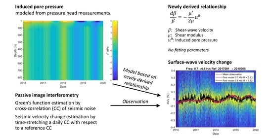
:Previous studies examining the relationship between the groundwater table and seismic velocities have been guided by empirical relationships only. Here, we develop a physics-based model relating fluctuations in groundwater table and pore pressure with seismic velocity variations through changes in effective stress. This model justifies the use of seismic velocity variations for monitoring of the pore pressure. Using a subset of the Groningen seismic network, near-surface velocity changes are estimated over a four-year period, using passive image interferometry. The same velocity changes are predicted by applying the newly derived theory to pressure-head recordings. It is demonstrated that the theory provides a close match of the observed seismic velocity changes.
1. Introduction
Seismic waves contain information about the subsurface; for instance, subsurface seismic properties such as shear modulus and density can be derived from observations of wave propagation. In Earth sciences, seismic data are therefore an important source of information. Relevant physical and chemical information can be found in seismic properties and especially in their variations. We distinguish two types of variations: spatial and time-lapse ones. Spatial variations in seismic velocity can indicate layer boundaries, faults or more subtle subsurface heterogeneity, e.g., [1]. Time-lapse variations in seismic velocity can be caused by changes in stress, temperature or composition.
A technique to retrieve time-lapse velocity variations is passive image interferometry [2]. This technique consists of two steps. First, the Green’s function is estimated using cross-correlations of seismic noise recorded at two receivers. Secondly, the cross-correlation result using, e.g., a day’s worth of data, is compared with a reference Green’s function to obtain the relative change in seismic velocity. This technique has been applied to find volcanic precursors [3], to monitor stress changes [4], ensure the safety of civil structures [5], and to monitor groundwater tables [6].
A groundwater table is the depth in the subsurface where the soil or rock is fully saturated with water. It is the border between the unsaturated upper part (vadose zone) and the lower phreatic zone. Over the seasons, the soil moisture in the vadose zone varies due to precipitation and evaporation. At the same time, the groundwater table fluctuates due to drainage and inundation. Changes in both zones affect the loading and pore pressure of the deeper subsurface. Locally, the pore pressure at depth can be measured with a piezometric well. For measurement over a larger region and depth range, recent developments in seismic methods are promising.
In many monitoring studies, the seismic velocity change is empirically linked to other observations, for which the velocity change is used as a measurement. For instance, Clements and Denolle [7] fitted seismic velocity changes linearly to changes in the groundwater table. This is also the case for other groundwater and pore pressure monitoring studies [2,6,7,8,9,10,11,12]. An empirical relationship between seismic velocity and the groundwater table or pore pressure can be useful, but without theory it cannot provide understanding on how seismic velocity changes are caused.
The Groningen region in the Netherlands has been a test bed for monitoring studies, both due to presence of a large seismic network [13] and pronounced changes in the subsurface due to gas extraction [14] and a thick layer of unconsolidated sediments [15]. The large azimuthal coverage of the network was used to test different quality parameters for passive image interferometry [16]. Moreover, seismic interferometry was applied to a string of geophones in the reservoir to measure compaction [17]. In another study, a dense surface network of stations was used to detect velocity changes in refracted waves over a one-month period [18]. Using the same dense array of 417 stations, a novel implementation of passive image interferometry was tested [19]. Following heavy rain, they found a velocity reduction that propagates downward with time. This they explained with effective-pressure diffusion.
This study provides a physics-based model connecting fluctuations in the pore pressure and vertical compressional stress to seismic velocity variations through changes in effective stress. We combine the relationship between induced stress and velocity change, derived from first principles by Tromp and Trampert [20], with wave propagation theory, basic hydrology and geomechanics to relate velocity change directly to fluctuations in the pore pressure and vertical compressional stress. Using data collected in Groningen, the Netherlands, we validate this relationship, and show that it enables us to monitor near surface (i.e., top 500 m) changes in pore pressure using passive image interferometry.
2. Theory
We derive a physics-based relationship between shear-wave velocity change and fluctuations in the groundwater table and pore pressure. First, we rewrite the existing relationship between seismic velocity and induced stress by Tromp and Trampert [20]. Then, we use basic hydrology and geomechanics to model the induced stress. Last, we study the relative contribution of different terms in the final equation. A similar derivation for compressional-wave velocity change can be found in Appendix A.
2.1. Velocity Change Due to Induced Stress
Relationships between seismic velocity and induced stress were derived from first principles by eq. 38 (Tromp and Trampert [20]). They showed that for an induced stress (defined as negative for compression), written in terms of an induced pressure and a symmetric trace-free induced deviatoric stress , the shear-wave velocity can be written as
with mass density , shear-wave velocity without induced stress, its perturbation due to induced stress, shear modulus , its pressure derivative , direction of propagation , and direction of motion . We rewrite this equation to find relative velocity change by subtracting from both sides of the equation
and dividing by :
Since velocity changes are usually small , this relationship can be approximated as
2.2. Velocity Change Due to Surface Load and Pore Pressure
Wherever pore pressure plays a role, poroelastic theory states that deformation is proportional to the effective stress, defined by p. 32 [21], where represents the Biot constant and u is the pore pressure. The solid framework carries the part of the total external stress , while the remaining part, , is carried by the fluid. An increase in pore pressure essentially reduces the forces on the contact surfaces between the grains (i.e., becomes less negative, since (effective) stress is defined as negative for compression). The remaining pore pressure, , is counteracted by internal stresses in the solid. In unconsolidated or weak material, is close to 1. We therefore need to formulate Equations (1)–(4) in terms of the effective stresses and the pore pressures that affect them.
We examine changes in effective stress that are induced by (near) surface processes such as fluctuation of the groundwater table or the atmospheric pressure. Such processes cause almost instant changes in the stress, while pore pressure diffusion is highly dependent on the permeability of the layers and viscosity of water. Therefore, we assume induced stress from surface processes to be independent of depth, while we allow induced pore pressure to vary with depth. In a one-dimensional model, this automatically satisfies the zero divergence condition . For the loading effect, we only consider changes in vertical stress .
We write the induced effective stress as
with corresponding induced effective pressure
and induced effective deviatoric stress
We distinguish three types of shear waves: shear waves with vertical propagation and horizontal motion (; ; ; ), shear waves with horizontal propagation and horizontal motion (; ; ; ), and shear waves with horizontal propagation and vertical motion (; ; ; ). Respectively, this simplifies Equation (8) to
and
3. Model Validation
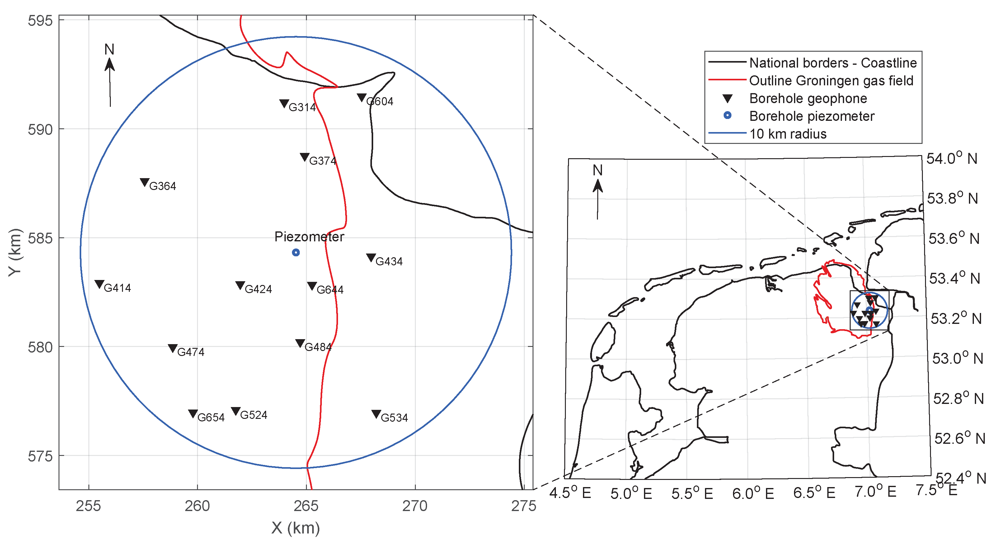
To validate the relationships derived in the previous section, we model surface-wave velocity changes based on pressure-head measurements and compare their results to independent measurements obtained with passive image interferometry. From pressure-head measurements, recorded by piezometer B08C0952 [22] in Groningen, the Netherlands (Figure 1), we estimated changes in pore pressure and vertical stress, which are used as inputs to Equations (9)–(11) to model shear-wave velocity changes. Corresponding surface-wave velocity changes were then obtained through surface-wave dispersion modeling. To obtain independent measurements of surface-wave phase-velocity changes, we applied passive image interferometry to seismic noise. To this end, we used seismic data from borehole geophones [23] at 200 m depth, located within a 10 km radius from the piezometer (Figure 1).
3.1. Static Model
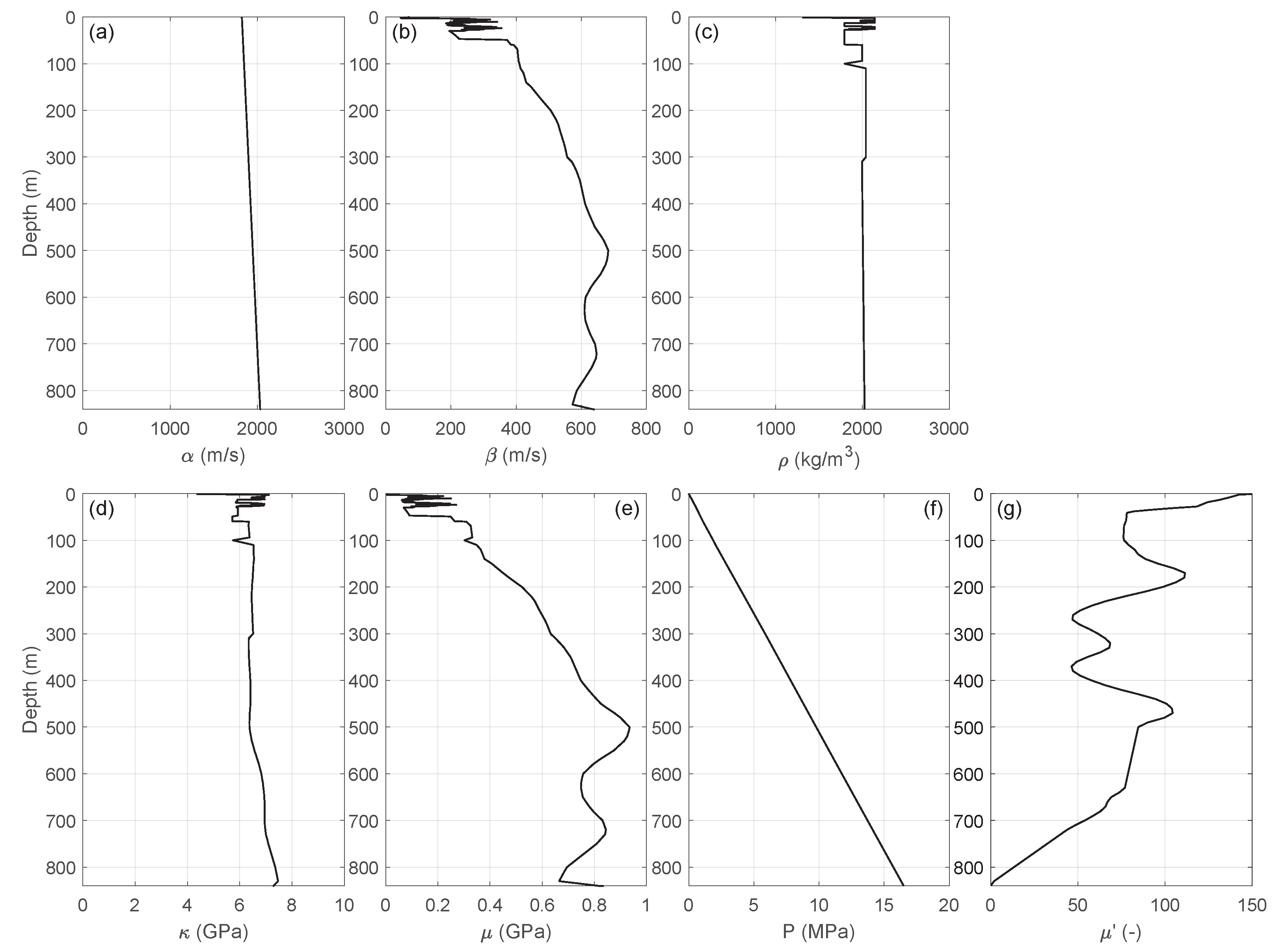
The static parameters in Equations (9)–(11) are and . They are estimated from detailed subsurface models available in the Groningen area. As a starting point, we used a local shear-wave velocity and density model from Kruiver et al. [24] and a compressional-wave velocity model from Romijn [25] at , visualized in Figure 2a–c. Note that the chosen model location below receiver G424 very close to the piezometer is a point location, whereas the used surface waves sample the entire region.
Using compressional-wave (a), shear-wave (b) and density models (c) we computed the bulk modulus (d), the shear modulus (e), and the confining pressure (f). A smoothed derivative of the shear modulus with respect to the confining pressure is shown in Figure 2g. Note that increases with depth, whereas decreases with depth. has values above 50 for most of the unconsolidated-sediment depth range (upper 800 m) and much smaller values for the underlying chalk rock.
3.2. Stress Model
The borehole piezometer shown in Figure 1 [22] has registered pressure heads (i.e., the levels to which groundwater rises in a frictionless tube due to pore pressure) at depths , , , , and m. Figure 3a shows the change in pressure head with respect to the average pressure head between 1 January 2017 and 31 December 2019. If there were a high permeability between the measurement depths , all measurements should be identical. Figure 3a shows this is not the case for depths m. This corresponds with the presence of low-permeability clay layers in this depth range.
From a linear interpolation of the pressure head, we obtained changes in pore pressure as a function of depth and time. values at the deepest three measurement levels are nearly identical. For that reason, we extrapolated below depths of 170.8 m as a constant with depth down to 840 m and set to zero for m, from where the sediments become consolidated. The resulting field is shown in Figure 3b for parameters kg/m3 and m/s2.
To estimate the order of magnitude of the induced vertical compressional stress, we assumed that changes in pressure head at the shallowest level are similar to changes in the groundwater table. Hence, we used m. Figure 3c shows the result for porosity .
3.3. Shear-Wave Velocity Change
To compare the effects of groundwater table loading and induced pore pressure on the seismic velocity, we studied the orders of magnitude that can be predicted using Equations (9)–(11). Typical values for stress and pore pressure can be found at 1 January 2018, when the induced compressional stress was estimated at Pa, and the average pore pressure was Pa. Using the information of Figure 2e,g ( and Pa) in Equations (9) and (11), we found, for the groundwater loading, a relative increase in shear-wave velocity , and we found a relative decrease in shear-wave velocity for the induced pore pressure . Since the effect of vertical compressional stress is considerably smaller than the pore pressure effect in our Groningen setting, and we have no accurate measurements of , we chose to neglect the effect of the vertical compressional stress. Hence, we simplify Equations (9)–(11) to
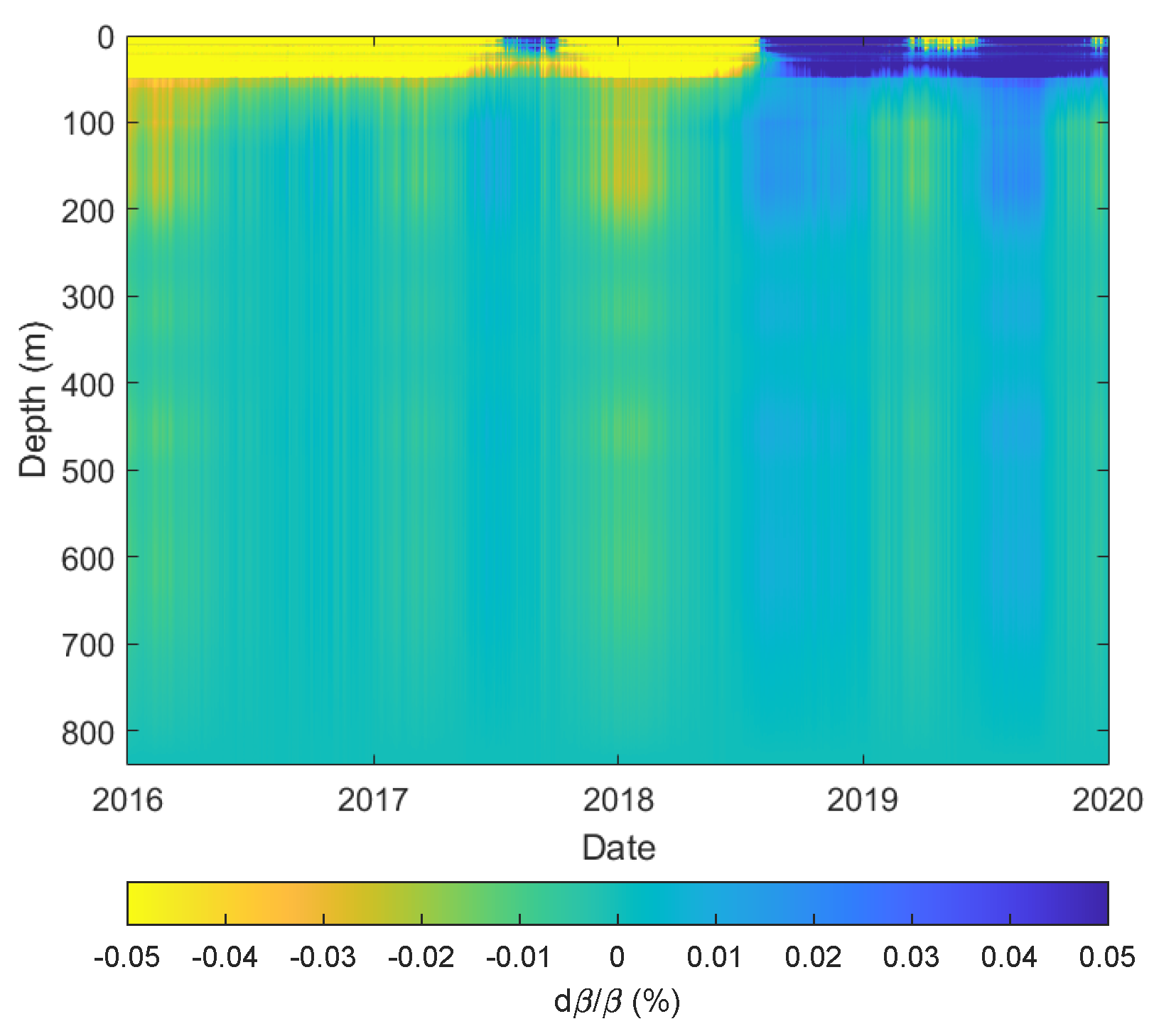
In accordance with Equation (12), we used the information from Figure 2e,g and Figure 3b to construct shear-wave velocity changes as a function of time and depth. The result in Figure 4 forms the basis in the forward modeling of surface-wave velocity changes. The effects of the pore pressure are mainly responsible for the time-lapse variations, while the shear modulus and its pressure derivative regulate the amplification of shear-wave velocity changes as a function of depth. For instance, at the interface at 50 m depth, the amplitude of velocity change rapidly decreases due to an increase in the shear modulus (Figure 2e), and a decrease in the pressure derivative of the shear modulus (Figure 2g).
3.4. Surface-Wave Dispersion Forward Modeling
Given our physics-based relationship regarding shear-wave velocity change as a function of depth (simplified as Equation (12)), and our observations of surface-wave phase velocity changes as a function of frequency (Section 3.5), we can relate them through surface-wave dispersion modeling. Assuming that the lateral variations in our region of interest are small, we can use a one-dimensional average static model of the subsurface and use the adjoint technique of Hawkins [26] to compute sensitivity kernels which relate partial derivatives of the change in surface-wave phase velocities (Love and Rayleigh) to the small stress-induced changes in shear-wave velocities. These partial derivatives can be used to estimate the effect on relative changes in surface-wave phase velocities using
where is the partial derivative of the surface-wave phase velocity with respect to at frequency , is the small perturbation to , and is the actual surface-wave phase velocity. While this approach is approximate and discounts the impact of anelasticity and lateral heterogeneity, it is sufficient to demonstrate that the stress-induced changes in shear-wave phase velocities give the correct changes in observed surface-wave velocities.
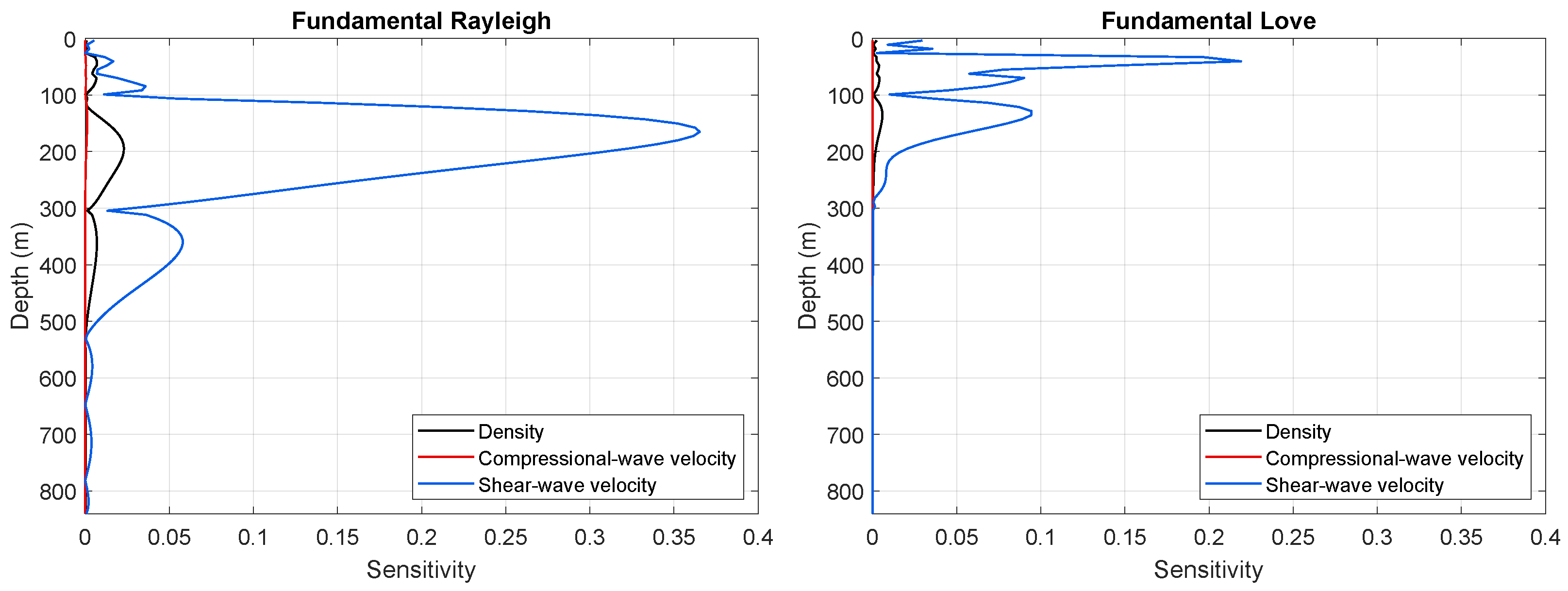
For the static models introduced in Section 3.1, we computed the sensitivity kernels of fundamental Rayleigh and Love waves for density, compressional-wave velocity and shear-wave velocity. Figure 5 shows the kernels at a frequency of 1 Hz. This figure shows that, in the Groningen setting, fundamental mode Love waves are more sensitive to shallower changes than Rayleigh waves, which peak around 200 m depth.
Figure 6 shows several eigen modes for Love and Rayleigh waves at 1 Hz, indicating that there should be reasonable amounts of Rayleigh-wave energy recorded at a depth of 200 m (depth of the borehole geophones we are going to use below), but little fundamental Love-wave energy. Overtones of both Love and Rayleigh will be recorded if excited by the seismic noise; however, our analysis suggests that the fundamental mode is dominant, at least in ZZ and TT cross-coherence’s (Figure 7), as shown in Figure 8.
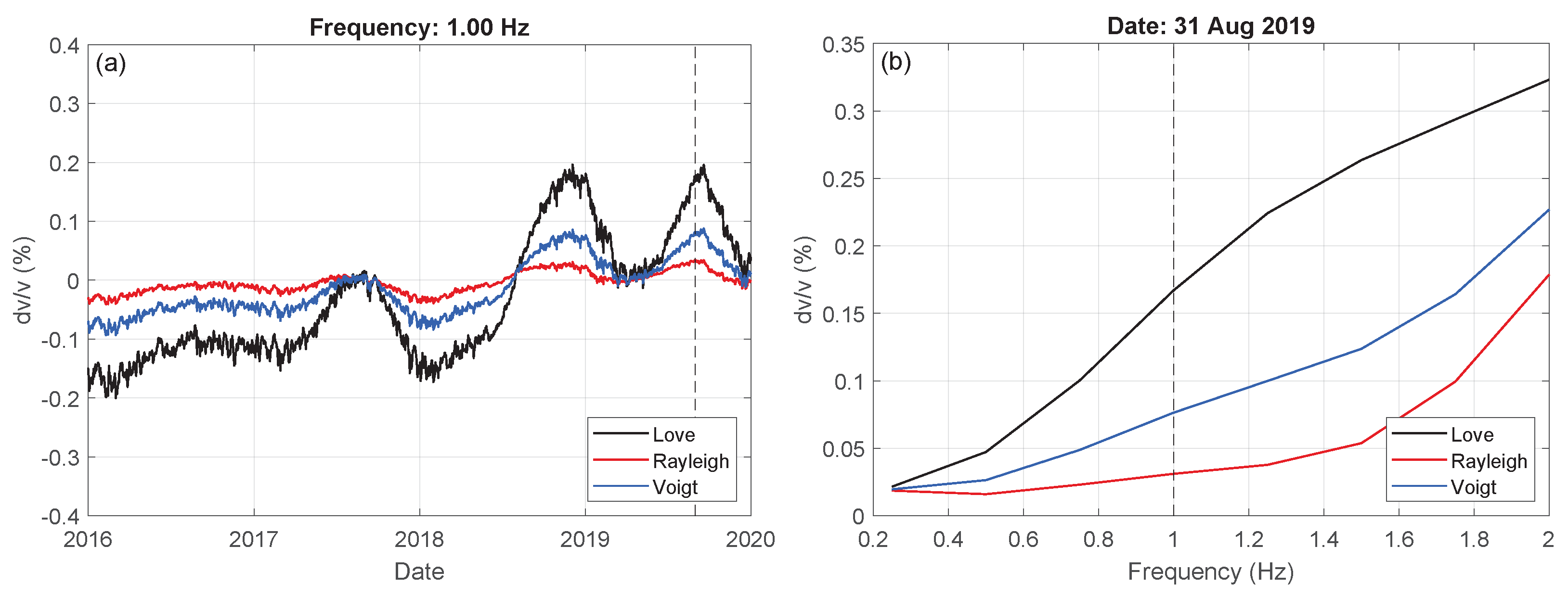
Using the adjoint method [26], we modeled surface-wave velocity changes corresponding to the shear-wave velocity changes shown in Figure 4. Figure 9 shows the relative velocity changes for the example frequency of 1 Hz as a function of date (a) and for the example date 31 Aug 2019 as a function of frequency (b). We show relative velocity change of Love waves (black), Rayleigh waves (red), and its Voigt average (blue). Love waves show a larger induced velocity change than Rayleigh waves. This can be understood from their higher sensitivity to shallow depths (Figure 5), where the largest shear-wave velocity changes occur (Figure 4). For low frequencies, we used the Voigt average of Rayleigh and Love waves, but higher frequencies (Figure 8) show less energy for Love waves than for Rayleigh waves. Therefore, we used Rayleigh wave velocity change for frequencies Hz, which has a much lower amplitude than the Voigt average.
3.5. Passive Image Interferometry
In an approach similar to Fokker and Ruigrok [16], building upon the work of Sens-Schönfelder and Wegler [2], we retrieved relative changes in the seismic velocity using passive image interferometry, consisting of two main processes. First, the time-varying Green’s functions between two seismic receivers were estimated. Second, these estimates were used to determine the relative changes in arrival time, corresponding to the relative changes in velocity.
To estimate a daily Green’s function (i.e., a one-day average of a Green’s function), we computed the cross-coherence, i.e., the spectrally normalized cross-correlation, [28] of ambient seismic noise, recorded by seismic receivers at and :
The frequency domain is indicated by a hat and the star denotes a complex conjugation. We stacked cross-coherences calculated from 50% overlapping time windows of 20 min durations, where the first time window ranges from 0:00 to 0:20 UTC, the second from 0:10 to 0:30 UTC, etc. We repeated this procedure for the data of every day between 1 January 2016 and 1 January 2020. The cross-coherences were computed for all component combinations. To speed up computation, we applied rotations to radial (R) and transverse (T) components after cross-correlation. Applying rotation after correlation gives a small yet acceptable error (Appendix B). Figure 7 shows the average cross-coherence between 1 January 2017 and 31 December 2019 as a function of distance between receivers. A different time period was chosen for the reference cross-coherence, since in 2016 quite a lot of data are missing. In this way, the reference cross-coherence contains equal contributions from all seasons, while available data from 2016 can still be compared to a well estimated Green’s function.
We determined velocity changes using the stretching method in the time domain [29]. Relative velocity changes were found at the maximum correlation coefficient between lapse (daily) cross-coherence , stretched in time with factor , and reference cross-coherence ,
The obtained velocity changes are relative to the reference cross-coherence, here defined as the average cross-coherence between 1 January 2017 and 31 December 2019 (Figure 7). We decided to only use the coda of the cross-coherence (red areas in Figure 7), because the coda is less dependent on changes in illumination, and velocity change causes larger changes in traveltime for late arrivals. This results in more accurate and stable measurements of the velocity change. As time windows (integration boundaries in Equation (15)) for the cross-coherence, we therefore used s s, where the first term is the distance x between the two receivers divided by the minimum expected propagation velocity. An additional 5 s was added to exclude the direct field with certainty. We applied bandpass filters to the cross-coherences, varying both the center frequency and the frequency span to obtain surface wave velocity changes as a function of frequency.
A disadvantage of the stretching method is spurious velocity changes when coda-wave amplitudes vary [30]. The use of a spectral normalization of the cross-correlation, the cross-coherence, limits amplitude variations, but when the ambient noise amplitudes are weaker than the normalization water level used, the amplitudes of the cross-coherence change, resulting in spurious arrivals. For this reason, we analyzed the velocity change distributions of 78 receiver pairs (Figure 1). Spurious arrivals can easily be spotted by an inconsistent distribution of velocity change. Figure 10 shows an example of an inconsistent distribution of velocity change. These spurious velocity changes can especially be observed during summers and at low frequencies ( Hz). During these seismically quiet periods, the 4.5 Hz geophones record a significant proportion of instrumental noise, which results in a poor estimate of Green’s function.
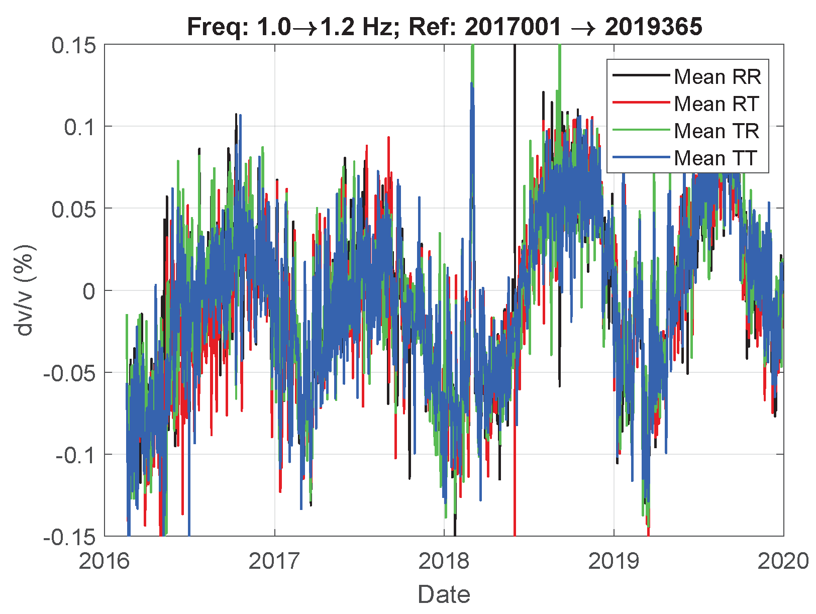
Employing coda waves measured on the horizontal components, we cannot distinguish between Rayleigh, Love and body waves, since the coda consists of multiply-scattered waves. To show that surface waves dominate the Groningen noise, we applied multichannel analysis of surface waves [27] to the reference cross-coherences, measured on the radial, vertical and transverse components. Figure 8 shows a strong presence of both Rayleigh and Love waves. The surface-wave dispersion can be seen up until about 1 Hz. The dispersion cannot be discerned at higher frequencies, probably due to the near-surface heterogeneity over the area sampled with the 78 receiver pairs (Figure 1). Since surface waves dominate Green’s function estimates (the cross-coherences), we treat the average velocity change in the coda for lower frequencies as the Voigt average of the Rayleigh and Love wave phase velocity changes, and for higher frequencies as Rayleigh wave phase velocity changes. Figure 11 shows that for the coda of the cross-coherence every horizontal component configuration (i.e., RR, RT, TR, TT) leads to similar velocity changes. This indicates that arrivals of both Love and Rayleigh waves can indeed be measured on the coda of all horizontal components. An average over all horizontal component configurations will lead to a cleaner distribution of velocity change. For the cross-coherence of vertical motion at both receivers, Rayleigh waves dominate. Hence, we treat velocity change obtained with coda waves recorded on the vertical component as phase velocity changes in the Rayleigh wave.
3.6. Model Validation
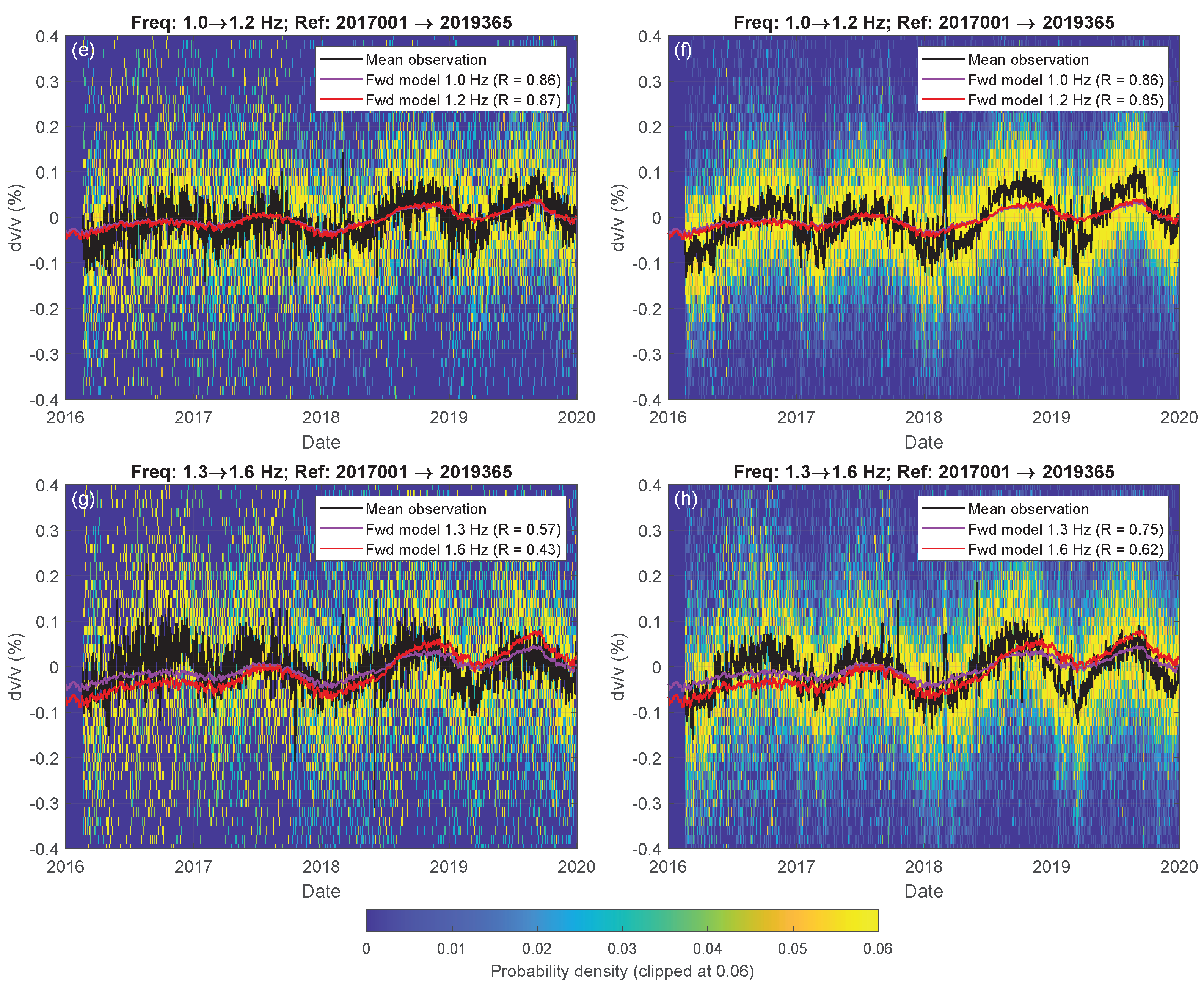
Relative seismic phase-velocity variations were retrieved for all combinations of the seismic receivers indicated in Figure 1 for frequency bandwidths of [0.3 0.4], [0.7 0.8], [1.0 1.2], and [1.3 1.6] Hz. Figure 12 presents the mean velocity change (black) and its distribution (colored background) of 78 station combinations of one vertical (ZZ; left) and four horizontal-component configurations (i.e., the average velocity change of components RR, RT, TR, TT; right). The observations of surface-wave velocity change (black) match the results of the independent forward model (purple and red) quite well, both in shape and magnitude. For the vertical component and the higher frequencies of the horizontal components, the Rayleigh-wave velocity-change model is shown. For the lower frequencies of the horizontal components, a Voigt average was taken over the Rayleigh and Love velocity-change models (Figure 9).
4. Discussion
To retrieve velocity variations of surface waves, we used the stretching method [29]. This method is based on the assumption that velocity change is homogeneous. This assumption is valid for velocity changes due to fluctuations in the pore pressure, because the causes of these fluctuations, i.e., precipitation and evaporation, are similar for the whole area. Local velocity changes, for which the assumption is not valid, cannot be retrieved using this method.
In a similar study, Fokker and Ruigrok [16] retrieved velocity variations in a region 15 km northwest of the area sampled in this study. Compared to their results, our velocity variations are three times smaller. This discrepancy can likely be explained by differences in depth sensitivity for fundamental modes and the overtones of Rayleigh waves, and the dominant amplitude of motion at 50 and 200 m depths. At a depth of 200 m, used in the present study, motion of the fundamental mode dominate over motion of the overtones (Figure 8). At a depth of 50 m, used by Fokker and Ruigrok [16], motion of the first overtone dominates over the motion of the fundamental mode. In Mordret et al. [19], it is shown that, in the Groningen setting, the first overtone of the Rayleigh wave has a higher sensitivity to velocity changes than the fundamental mode.
Note that, for some frequencies, we observed the first Rayleigh overtone on the RR component (Figure 8), while we used the fundamental mode in the modeling (Figure 9 and Figure 12). The match between model and observation will likely improve when overtones are included.
In our model for velocity change, we excluded the Love wave contribution for frequencies Hz due to the low Love-wave energy (Figure 8) and its relatively small amplitude at 200 m depth (Figure 6). If the Voigt average (Figure 9 blue) was taken at these higher frequencies, the amplitude of the velocity change model would be much higher. The Voigt averaged model for velocity change would overestimate the velocity change observations at higher frequencies (Figure 12f,h).
In our stress model (Section 3.2), we interpolated the change in pressure head between the measurement depths, we extrapolated as uniform changes between 170.8 m and 840 m depth, and we assumed no changes below the consolidation interface at 840 m depth. We expected the permeability to decrease at this interface, limiting the changes in pore pressure. However, pore pressure changes at depths below 840 m depth are not relevant for the purpose of this study, since the waves we study have no sensitivity to changes at depths below 500 m (Figure 5).
We observed that some studies found a positive correlation between groundwater fluctuations and velocity changes [6,11], while others found an anti-correlation [2,7,8,31,32]. This can be explained by the different mechanisms presented in Section 2. The contributions of and in Equations (9) and (11) have opposite effects: an increase in pore pressure results in a decrease in seismic velocity, while an increase in compressional stress ( becomes more negative) results in an increase in seismic velocity. The balance between the mechanisms depends, on the one hand, on the permeability determining the size of , relative to . On the other hand, it depends on the presence of Rayleigh and Love waves, and their responses to changes in S-wave velocities. Both negative and positive correlations with, respectively, pore pressure and surface weight were found by Wang et al. [10], who modeled the pore pressure from precipitation measurements and used measurements of snow depth for surface loading.
This article argues that shear-wave velocity changes are caused by fluctuations of the effective stress through changes in the shear modulus. There is, however, a second mechanism to couple velocity change to induced effective stress. Effective pressure leads to compaction, affecting the density and hence the shear-wave velocity. This effect can be quantified using the density derivative of the shear-wave velocity, , and the definition of the Bulk modulus, . A rise in effective pressure would induce a relative change in density , resulting in an increase in shear-wave velocity . For a typical bulk modulus in the Groningen subsurface, Pa (Figure 2d), this would result in velocity changes that are two to three orders of magnitude smaller than the ones observed. Therefore, we neglected the mechanism of compaction.
This study focuses on seismic velocity changes due to changes in the pore pressure. Here, we address sources for velocity changes that could not have been measured due to our choices for surface waves, frequency bandwidths, temporal resolution and methodology.
In some studies, atmospheric temperature variations are correlated to seismic velocity change, e.g., [33]. The temperature oscillations in the subsurface, due to yearly atmospheric temperature variations, can mathematically be described as a highly damped wave propagating downwards. Most of the effect is located above 20 m. For depths below 20 m, the temperature changes for quartz, with a thermal diffusivity mm2/s, would be limited to 0.1 °C. The surface waves, with frequencies we used, have no sensitivity to changes at depths shallower than 20 m (Figure 5). Furthermore, surface waves are sensitive to changes over a large range of depths, while the wavelength of the thermal “wave” is approximately 25 m, resulting in temperature contributions of a range of seasons. This would not be detectable using surface waves at frequencies lower than 2 Hz.
Velocity changes caused by the Lunar tides were also left out, because we have only one velocity measurement per day, whereas Lunar tides cause two oscillations of velocity change per day. Velocity changes induced by Groningen earthquakes (maximum magnitude 3.4, at 3 km depth) would not be detectable due to the relatively small induced stress in the shallow subsurface and the heterogeneous nature of the velocity changes. Changes in water saturation are not relevant as a potential source either, since these changes can only be observed above the groundwater table, which around Groningen is at a depth of approximately 1 m.
The derived relationship between shear-wave velocity and induced effective stress is validated in the context of surface waves, traveling through the shallow subsurface of the Earth. It provides a new understanding of time-lapse variations in the subsurface. We postulate that it can be directly applied to monitoring studies using shear waves or compressional waves (Appendix A) and may provide new insights in monitoring civil structures.
5. Conclusions
In this study, we developed a theory relating seismic velocity change to fluctuations in the pore pressure and vertical stress. By combining a relationship between seismic velocity and induced stress, derived from first principles [20], with basic hydrology and geomechanics, we derived a physics-based relationship for seismic velocity changes as a function of induced pore pressure, vertical compressional stress and elastic parameters. To validate this relationship, we modeled seismic surface-wave velocity changes, based on measurements of the pressure head, using the newly derived relationship and the adjoint method [26]. Surface-wave velocity changes were independently retrieved by applying passive image interferometry [2] to seismic noise measured in the subsurface of Groningen, the Netherlands. The close match between model and observation shows the validity of the derived theory, and justifies the use of seismic velocity variations for pore pressure monitoring.
Author Contributions
Conceptualization, E.F., E.R. and J.T.; methodology, E.F., E.R., R.H. and J.T.; software, E.F. and R.H.; validation, E.F.; formal analysis, E.F.; investigation, E.F.; resources, E.R. and J.T.; data curation, E.F.; writing—original draft preparation, E.F.; writing—review and editing, E.R., R.H. and J.T.; visualization, E.F.; supervision, E.R. and J.T.; project administration, E.F.; funding acquisition, J.T. All authors have read and agreed to the published version of the manuscript.
Funding
This work is part of research programme DeepNL, financed by the Dutch Research Council (NWO) under project number DeepNL.2018.033.
Institutional Review Board Statement
Not applicable.
Informed Consent Statement
Not applicable.
Data Availability Statement
The seismic and pressure-head data is openly available at http://rdsa.knmi.nl/network/NL/, accessed on 31 May 2021, and https://www.dinoloket.nl/ondergrondgegevens, accessed on 31 May 2021, respectively. Data files pertaining to the different figures can be requested from the corresponding author.
Acknowledgments
The authors thank Fulco Teunissen for his constructive suggestions, which improved the manuscript, and Thomas Cullison for his programming insights and suggestions. We thank Hanneke Paulssen and Janneke de Jong for their input during our weekly meetings. Three anonymous reviewers provided helpful comments and suggestions for which we are also grateful.
Conflicts of Interest
The authors declare no conflict of interest.
Appendix A. Stress-Induced Compressional-Wave Velocity Change
Appendix B. Rotation Approximation
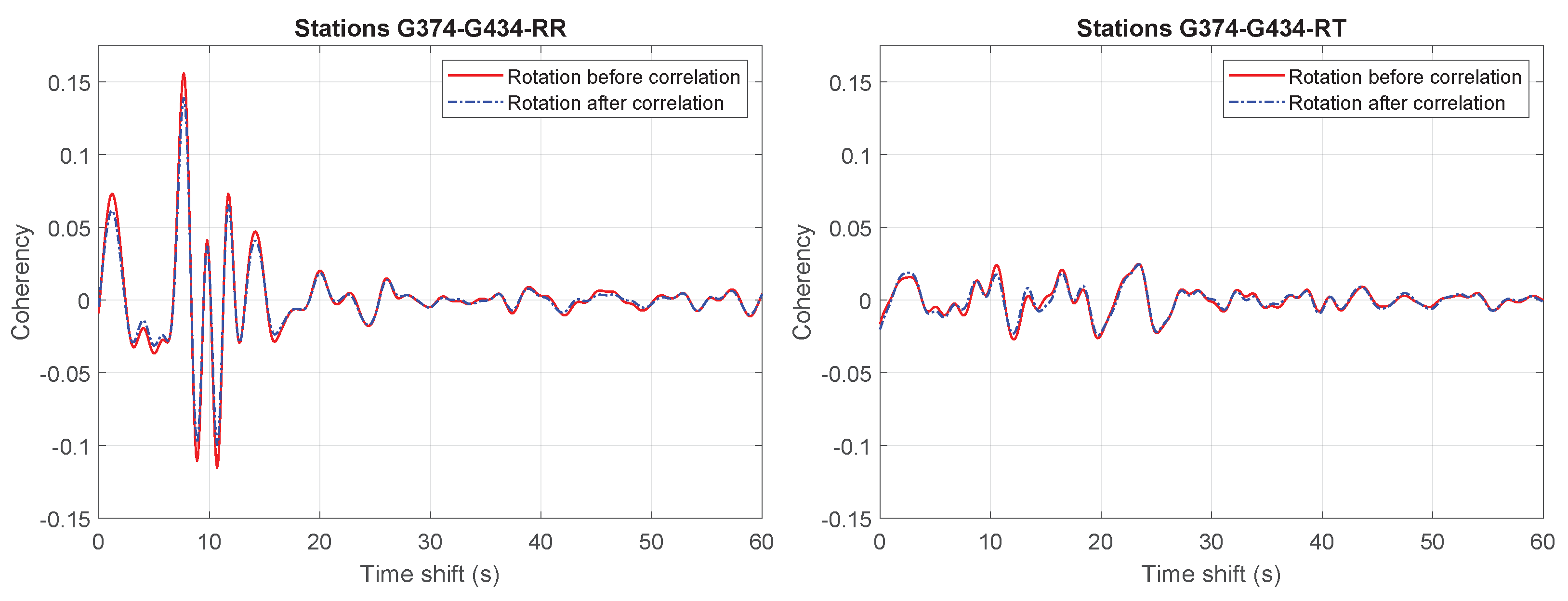
For the estimation of the Green’s function in the radial and transverse directions, we need to rotate the seismic measurements to face these directions. Traditionally, this is carried out before a cross-correlation is made. However, the data that are stored after cross-correlation are only a fraction of the raw data. For this reason, the computation time can be significantly reduced when the rotation is carried out after the cross-correlation. In this appendix, we assess the error that is introduced by applying rotation after cross-correlation.
A cross-correlation of radial–radial components can, in the frequency domain, be written as
where represents motion at location in the radial direction, represents the clockwise angle between the station orientation (i.e., the line between and ) and the North, and denotes the cross-correlation between the motion at in the northern direction and at in the eastern direction. Similarly, we find
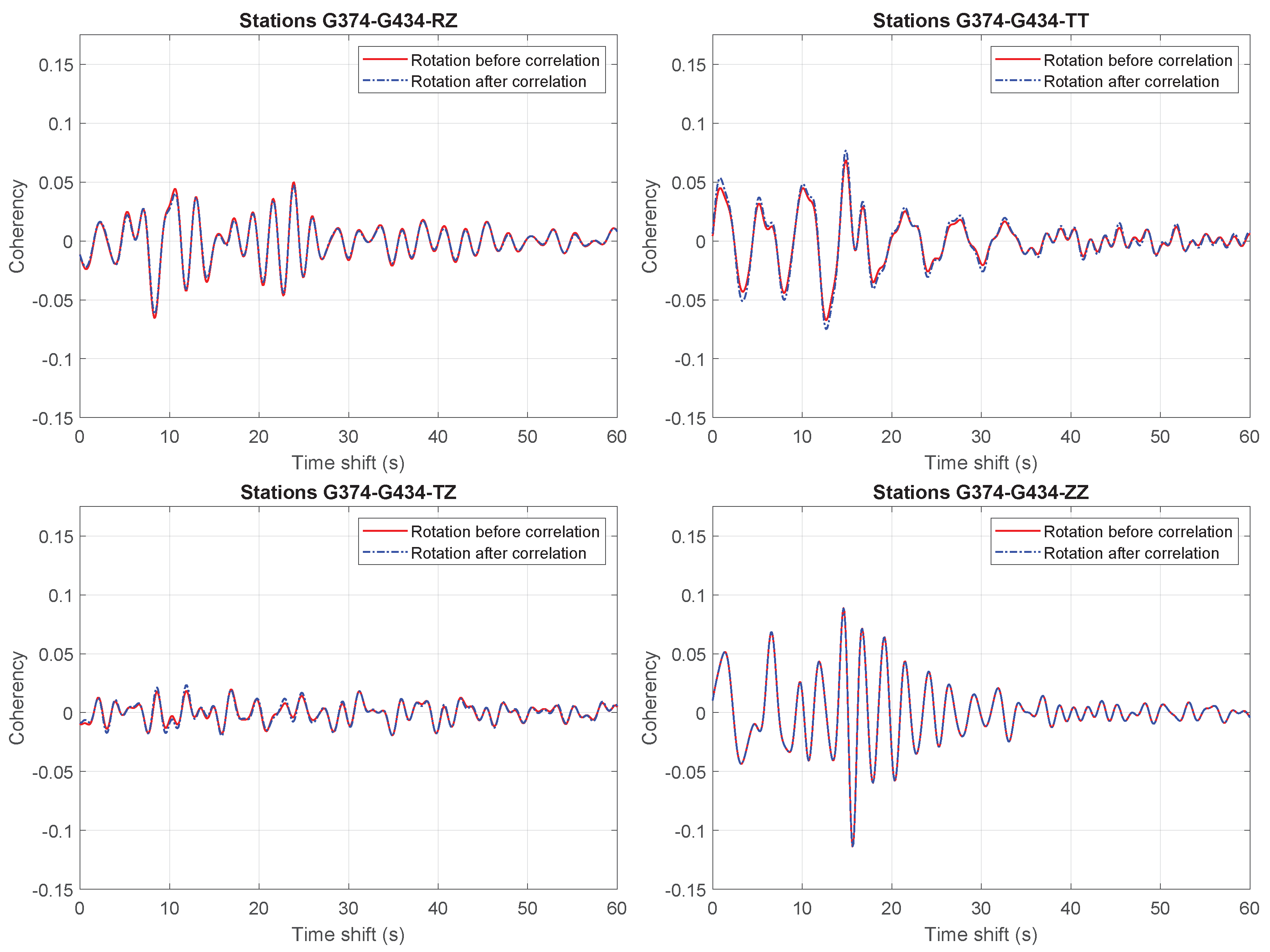
If no normalization has been applied both in the time and frequency domains, the result should be identical if the rotation was applied before or after the cross-correlation. This we indeed observed. When spectral whitening is applied, however, differences are expected, because the spectra of Rayleigh and Love waves are not identical. If the rotation is then applied after the cross-correlation, the spectral whitening allows for leakage of Love-wave energy to the radial cross-correlation, and Rayleigh-wave energy to the transverse cross-correlation. This effect is quantified for the geophone combination shown in Figure A1.
For rotations to components RR, RT, TR and TT, the differences are the largest, because the rotations are carried out in two steps using combinations of components NN, NE, EN and EE. Still, the phase differences are minimal, and the differences in amplitude are acceptable. The same applies for components RZ, TZ, ZR and ZT, in which only one rotation step is applied and where the differences are smaller. Component ZZ does not require a rotation and is therefore not affected by the processing order.
Furthermore, for the purpose of velocity variation estimation, leakage of Rayleigh and Love wave energy to orthogonal components is not relevant, because the direct wave is not used. In arrivals of (multiply) reflected surface waves i.e., surface waves that have reflected multiple times, leakage takes place anyway. Therefore, in this study, we did not apply rotation until after cross-correlation.
Figure A1.
Comparison of applying rotation before or after cross-correlation using spectral normalization for different component combinations and for receiver pair G374–G434.
Figure A1.
Comparison of applying rotation before or after cross-correlation using spectral normalization for different component combinations and for receiver pair G374–G434.


References
- Rawlinson, N.; Fichtner, A.; Sambridge, M.; Young, M.K. Chapter One—Seismic Tomography and the Assessment of Uncertainty. Adv. Geophys. 2014, 55, 1–76. [Google Scholar] [CrossRef]
- Sens-Schönfelder, C.; Wegler, U. Passive image interferometry and seasonal variations of seismic velocities at Merapi Volcano, Indonesia. Geophys. Res. Lett. 2006, 33. [Google Scholar] [CrossRef]
- Brenguier, F.; Shapiro, N.M.; Campillo, M.; Ferrazzini, V.; Duputel, Z.; Coutant, O.; Nercessian, A. Towards forecasting volcanic eruptions using seismic noise. Nat. Geosci. 2008, 1, 126. [Google Scholar] [CrossRef] [Green Version]
- Wegler, U.; Nakahara, H.; Sens-Schönfelder, C.; Korn, M.; Shiomi, K. Sudden drop of seismic velocity after the 2004 Mw 6.6 mid-Niigata earthquake, Japan, observed with Passive Image Interferometry. J. Geophys. Res. Solid Earth 2009, 114. [Google Scholar] [CrossRef]
- Salvermoser, J.; Hadziioannou, C.; Stähler, S.C. Structural monitoring of a highway bridge using passive noise recordings from street traffic. J. Acoust. Soc. Am. 2015, 138, 3864–3872. [Google Scholar] [CrossRef] [PubMed]
- Voisin, C.; Guzmán, M.A.R.; Réfloch, A.; Taruselli, M.; Garambois, S. Groundwater Monitoring with Passive Seismic Interferometry. J. Water Resour. Prot. 2017, 9, 1414–1427. [Google Scholar] [CrossRef] [Green Version]
- Clements, T.; Denolle, M.A. Tracking groundwater levels using the ambient seismic field. Geophys. Res. Lett. 2018, 45, 6459–6465. [Google Scholar] [CrossRef] [Green Version]
- Nakata, N.; Snieder, R. Estimating near-surface shear wave velocities in Japan by applying seismic interferometry to KiK-net data. J. Geophys. Res. Solid Earth 2012, 117. [Google Scholar] [CrossRef] [Green Version]
- Rivet, D.; Brenguier, F.; Cappa, F. Improved detection of preeruptive seismic velocity drops at the Piton de La Fournaise volcano. Geophys. Res. Lett. 2015, 42, 6332–6339. [Google Scholar] [CrossRef] [Green Version]
- Wang, Q.Y.; Brenguier, F.; Campillo, M.; Lecointre, A.; Takeda, T.; Aoki, Y. Seasonal crustal seismic velocity changes throughout Japan. J. Geophys. Res. Solid Earth 2017, 122, 7987–8002. [Google Scholar] [CrossRef]
- Liu, C.; Aslam, K.; Daub, E. Seismic Velocity Changes Caused by Water Table Fluctuation in the New Madrid Seismic Zone and Mississippi Embayment. J. Geophys. Res. Solid Earth 2020, 125, e2020JB019524. [Google Scholar] [CrossRef]
- Andajani, R.D.; Tsuji, T.; Snieder, R.; Ikeda, T. Spatial and temporal influence of rainfall on crustal pore pressure based on seismic velocity monitoring. Earth Planets Space 2020, 72, 1–17. [Google Scholar] [CrossRef]
- Dost, B.; Ruigrok, E.; Spetzler, J. Development of seismicity and probabilistic hazard assessment for the Groningen gas field. Neth. J. Geosci. 2017, 96, s235–s245. [Google Scholar] [CrossRef] [Green Version]
- Van Eijs, R.M.; van der Wal, O. Field-wide reservoir compressibility estimation through inversion of subsidence data above the Groningen gas field. Neth. J. Geosci. 2017, 96, s117–s129. [Google Scholar] [CrossRef] [Green Version]
- Van Ginkel, J.; Ruigrok, E.; Herber, R. Using horizontal-to-vertical spectral ratios to construct shear-wave velocity profiles. Solid Earth 2020, 11, 2015–2030. [Google Scholar] [CrossRef]
- Fokker, E.B.; Ruigrok, E.N. Quality parameters for passive image interferometry tested at the Groningen network. Geophys. J. Int. 2019, 218, 1367–1378. [Google Scholar] [CrossRef]
- Zhou, W.; Paulssen, H. Compaction of the Groningen gas reservoir investigated with train noise. Geophys. J. Int. 2020, 223, 1327–1337. [Google Scholar] [CrossRef]
- Brenguier, F.; Courbis, R.; Mordret, A.; Campman, X.; Boué, P.; Chmiel, M.; Takano, T.; Lecocq, T.; Van der Veen, W.; Postif, S.; et al. Noise-based ballistic wave passive seismic monitoring. Part 1: Body waves. Geophys. J. Int. 2020, 221, 683–691. [Google Scholar] [CrossRef] [Green Version]
- Mordret, A.; Courbis, R.; Brenguier, F.; Chmiel, M.; Garambois, S.; Mao, S.; Boué, P.; Campman, X.; Lecocq, T.; Van der Veen, W.; et al. Noise-based ballistic wave passive seismic monitoring–Part 2: Surface waves. Geophys. J. Int. 2020, 221, 692–705. [Google Scholar] [CrossRef]
- Tromp, J.; Trampert, J. Effects of induced stress on seismic forward modelling and inversion. Geophys. J. Int. 2018, 213, 851–867. [Google Scholar] [CrossRef]
- Fjar, E.; Holt, R.M.; Raaen, A.; Horsrud, P. Petroleum Related Rock Mechanics; Elsevier: Amsterdam, The Netherlands, 2008. [Google Scholar]
- Dinoloket. Groundwater Research; Borehole Identification B08C0952. 2020. Available online: https://www.dinoloket.nl/ondergrondgegevens (accessed on 5 June 2020).
- KNMI. Netherlands Seismic and Acoustic Network. Royal Netherlands Meteorological Institute (KNMI), Other/Seismic Network, 1993. Available online: http://rdsa.knmi.nl/network/NL/ (accessed on 16 May 2020). [CrossRef]
- Kruiver, P.P.; van Dedem, E.; Romijn, R.; de Lange, G.; Korff, M.; Stafleu, J.; Gunnink, J.L.; Rodriguez-Marek, A.; Bommer, J.J.; van Elk, J.; et al. An integrated shear-wave velocity model for the Groningen gas field, The Netherlands. Bull. Earthq. Eng. 2017, 15, 3555–3580. [Google Scholar] [CrossRef] [Green Version]
- Romijn, R. Groningen Velocity Model 2017; Technical Report; Nederlandse Aardolie Maatschappij: Assen, The Netherlands, 2017. [Google Scholar]
- Hawkins, R. A spectral element method for surface wave dispersion and adjoints. Geophys. J. Int. 2018, 215, 267–302. [Google Scholar] [CrossRef]
- Park, C.B.; Miller, R.D.; Xia, J. Imaging dispersion curves of surface waves on multi-channel record. In Proceedings of the 1998 SEG Annual Meeting; Society of Exploration Geophysicists: Salt Lake City, UT, USA, 1998. [Google Scholar] [CrossRef]
- Wapenaar, K.; Slob, E.; Snieder, R.; Curtis, A. Tutorial on seismic interferometry: Part 2—Underlying theory and new advances. Geophysics 2010, 75, 75A211–75A227. [Google Scholar] [CrossRef] [Green Version]
- Lobkis, O.I.; Weaver, R.L. Coda-wave interferometry in finite solids: Recovery of P-to-S conversion rates in an elastodynamic billiard. Phys. Rev. Lett. 2003, 90, 254302. [Google Scholar] [CrossRef]
- Zhan, Z.; Tsai, V.C.; Clayton, R.W. Spurious velocity changes caused by temporal variations in ambient noise frequency content. Geophys. J. Int. 2013, 194, 1574–1581. [Google Scholar] [CrossRef] [Green Version]
- Tsai, V.C. A model for seasonal changes in GPS positions and seismic wave speeds due to thermoelastic and hydrologic variations. J. Geophys. Res. Solid Earth 2011, 116. [Google Scholar] [CrossRef] [Green Version]
- Hillers, G.; Campillo, M.; Ma, K.F. Seismic velocity variations at TCDP are controlled by MJO driven precipitation pattern and high fluid discharge properties. Earth Planet. Sci. Lett. 2014, 391, 121–127. [Google Scholar] [CrossRef]
- Mao, S.; Campillo, M.; van der Hilst, R.D.; Brenguier, F.; Stehly, L.; Hillers, G. High Temporal Resolution Monitoring of Small Variations in Crustal Strain by Dense Seismic Arrays. Geophys. Res. Lett. 2019, 46, 128–137. [Google Scholar] [CrossRef] [Green Version]
Figure 1.
Map view of the locations of the measurement equipment employed in this study. The location of the piezometer B08C0952 [22] is plotted as a blue point, around which the blue circle indicates a 10 km radius. All geophones within this radius at 200 m depth [23] are shown as black triangles. The outline of the Netherlands and the Groningen gas field are shown as black and red lines.

Figure 2.
Static models: (a) Compressional-wave velocity , (b) shear-wave velocity , (c) mass density , (d) bulk modulus , (e) shear modulus , (f) confining pressure , with g the gravitational acceleration and z the depth below surface, (g) the shear-modulus pressure derivative , based on the smoothed derivative of the shear modulus with respect to confining pressure.

Figure 3.
(a) Time-lapse changes in pressure head with respect to the average pressure head between 1 January 2017 and 31 December 2019, for = , , , , and m depths. (b) Induced pore pressure = for parameters = 1000 kg/m3 and g = 9.8 m/s2, obtained from linear interpolation of . The dashed lines indicate the measurement depths of the pressure head. (c) Estimate of induced vertical compressional stress m for .
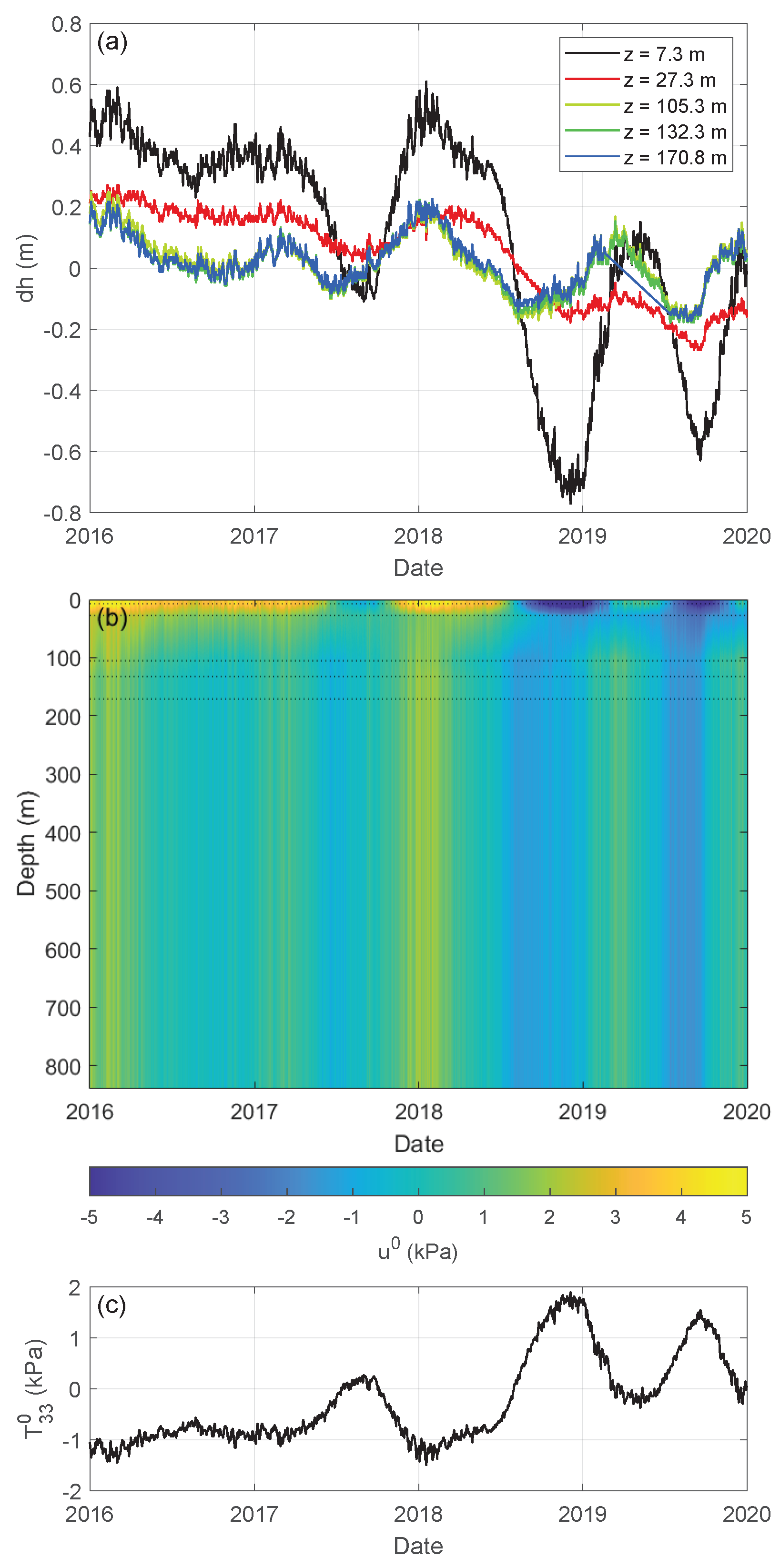
Figure 4.
Modeled shear—wave velocity change in accordance with Equation (12) and Figure 2e,g and Figure 3b.

Figure 5.
Absolute value of the sensitivity kernels for fundamental Rayleigh and Love waves for density, compressional-wave velocity and shear-wave velocity at a frequency of 1 Hz.
Figure 5.
Absolute value of the sensitivity kernels for fundamental Rayleigh and Love waves for density, compressional-wave velocity and shear-wave velocity at a frequency of 1 Hz.

Figure 6.
Eigen-mode amplitudes as function of depth for Rayleigh waves (amplitudes of both the horizontal and vertical components normalized to preserve amplitude ratios) and Love waves at 1 Hz.
Figure 6.
Eigen-mode amplitudes as function of depth for Rayleigh waves (amplitudes of both the horizontal and vertical components normalized to preserve amplitude ratios) and Love waves at 1 Hz.
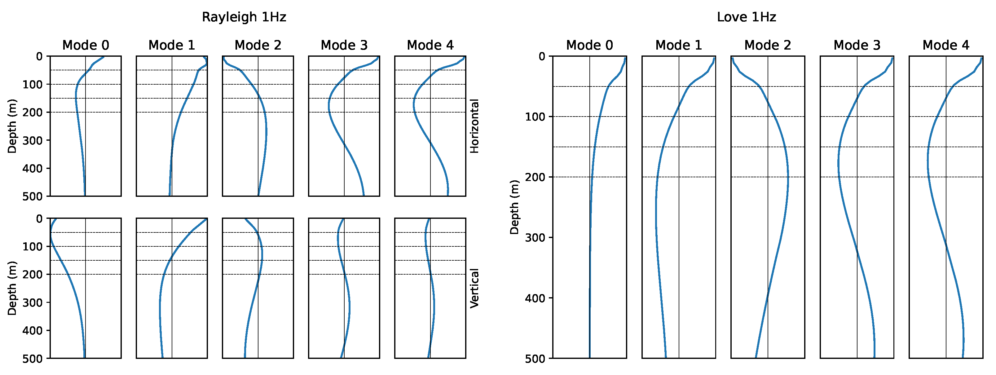
Figure 7.
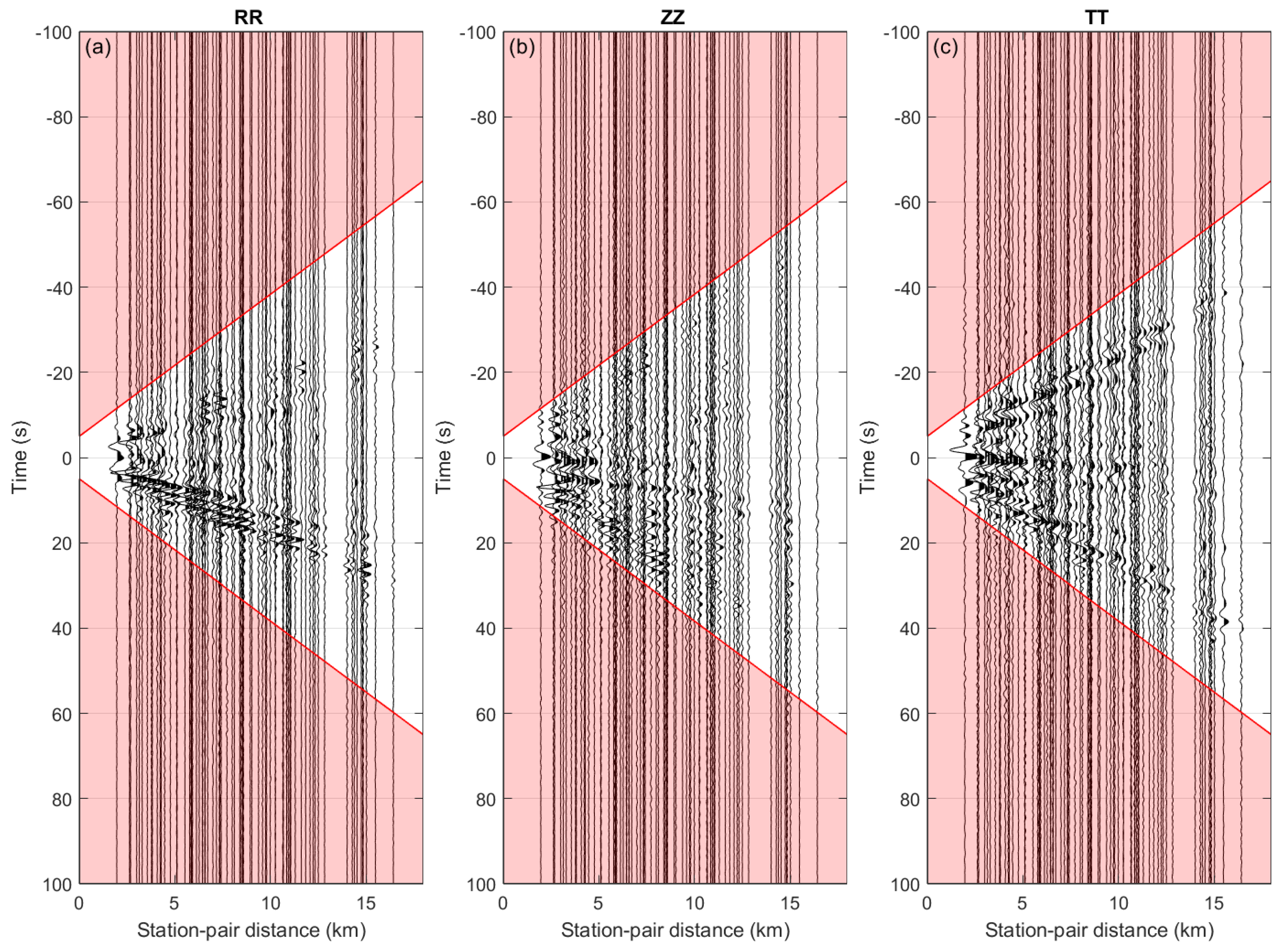
Reference cross-coherence (i.e., average cross-coherence between 1 January 2017 and 31 December 2019) for all combinations of receivers shown in Figure 1 as a function of receiver-pair distance for components (a) RR, (b) ZZ and (c) TT. The red lines indicate the arrival times , between which we expect all arrivals of direct surface waves, while the red area indicates the coda time windows s s, used in Equation (15) to retrieve relative velocity change.
Figure 7.
Reference cross-coherence (i.e., average cross-coherence between 1 January 2017 and 31 December 2019) for all combinations of receivers shown in Figure 1 as a function of receiver-pair distance for components (a) RR, (b) ZZ and (c) TT. The red lines indicate the arrival times , between which we expect all arrivals of direct surface waves, while the red area indicates the coda time windows s s, used in Equation (15) to retrieve relative velocity change.

Figure 8.
Multichannel analysis of surface waves [27] of the reference cross-coherences shown in Figure 7 for components (a) RR, (b) ZZ, and (c) TT, visualized in a power plot. The red lines indicate the fundamental dispersion curves of (a,b) Rayleigh and (c) Love waves, obtained with the adjoint method [26].
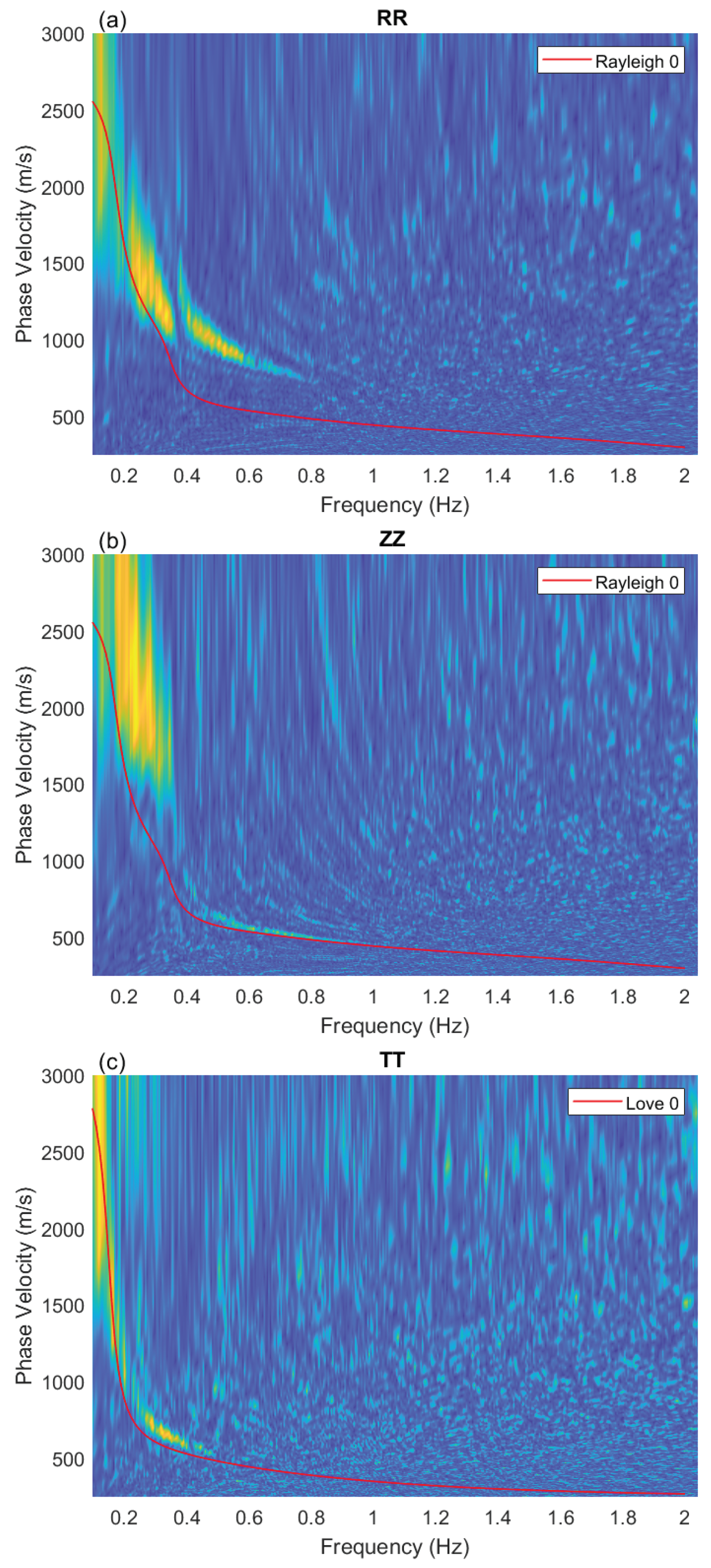
Figure 9.
(a) Modeled surface-wave velocity changes, for example, frequency 1 Hz as a function of date, and (b) for the example date 31 August 2019 as a function of frequency. The individual lines represent velocity change in Love waves (black), Rayleigh waves (red) and their Voigt average (blue).
Figure 9.
(a) Modeled surface-wave velocity changes, for example, frequency 1 Hz as a function of date, and (b) for the example date 31 August 2019 as a function of frequency. The individual lines represent velocity change in Love waves (black), Rayleigh waves (red) and their Voigt average (blue).

Figure 10.
Time-lapse seismic velocity change retrieved from seismic ambient noise within frequency bandwidth [0.1 0.2] Hz, using the coda of the cross-coherence of horizontal (RR, RT, TR, TT) components between 78 receiver combinations. The background colors show the probability distribution of 312 estimates from dark blue (low probability) to yellow (high probability), while the black line shows the average velocity change.
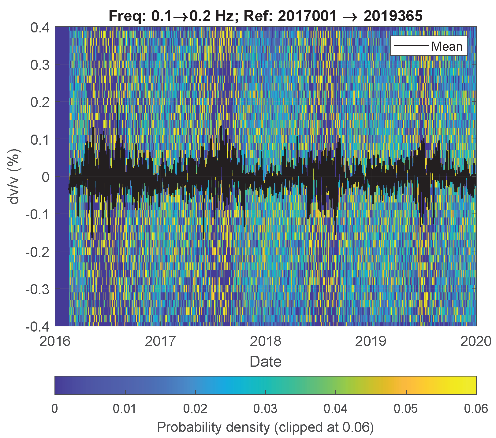
Figure 11.
Time–lapse seismic velocity change retrieved from seismic ambient noise within frequency bandwidth [1.0 1.2] Hz, using the coda of the cross-coherence of individual horizontal component configurations, averaged over 78 receiver combinations.
Figure 11.
Time–lapse seismic velocity change retrieved from seismic ambient noise within frequency bandwidth [1.0 1.2] Hz, using the coda of the cross-coherence of individual horizontal component configurations, averaged over 78 receiver combinations.

Figure 12.
Time–lapse seismic velocity change retrieved from seismic ambient noise within the indicated frequency bandwidths, using the coda of the cross-coherence of vertical (left; ZZ) and horizontal (right; RR, RT, TR, TT) components between 78 receiver combinations. The background colors show the probability distribution of 78 (left) and 312 (right) estimates from dark blue (low probability) to yellow (high probability), while the black line shows the average velocity change. The purple and red lines show the results of the independent forward model for velocity change of Rayleigh waves (a,c,e,f,g,h) and the Voigt average (b,d) as in Figure 9. The match between the low-frequency trends of the modeled and the observed velocity change was quantified with a Pearson correlation after a low-pass filter was applied with a cut-off period of 60 days. The correlation coefficient R is shown in the legend.

Publisher’s Note: MDPI stays neutral with regard to jurisdictional claims in published maps and institutional affiliations. |
© 2021 by the authors. Licensee MDPI, Basel, Switzerland. This article is an open access article distributed under the terms and conditions of the Creative Commons Attribution (CC BY) license (https://creativecommons.org/licenses/by/4.0/).
Share and Cite
MDPI and ACS Style
Fokker, E.; Ruigrok, E.; Hawkins, R.; Trampert, J. Physics-Based Relationship for Pore Pressure and Vertical Stress Monitoring Using Seismic Velocity Variations. Remote Sens. 2021, 13, 2684. https://doi.org/10.3390/rs13142684
AMA Style
Fokker E, Ruigrok E, Hawkins R, Trampert J. Physics-Based Relationship for Pore Pressure and Vertical Stress Monitoring Using Seismic Velocity Variations. Remote Sensing. 2021; 13(14):2684. https://doi.org/10.3390/rs13142684
Chicago/Turabian StyleFokker, Eldert, Elmer Ruigrok, Rhys Hawkins, and Jeannot Trampert. 2021. "Physics-Based Relationship for Pore Pressure and Vertical Stress Monitoring Using Seismic Velocity Variations" Remote Sensing 13, no. 14: 2684. https://doi.org/10.3390/rs13142684
Note that from the first issue of 2016, this journal uses article numbers instead of page numbers. See further details here.