Elevation Calculation of Bottom Deck Based on Stochastic Process and Compound Distribution

Abstract

In the design of offshore platforms, the height of the bottom deck directly affects the safety and engineering cost of the entire platform. It is a very important scale parameter in platform planning. The American Petroleum Institute (API) specification shows that the key to determining the height of the bottom deck lies in the wave height and calculation of the return level of the water increase. Based on the perspective of stochastic processes, this paper constructs a new distribution function model for joint parameter estimation of the marine environment. The new model uses a family of random variables to show the statistical characteristics of design wave height and water increase in both time and space, with extreme value expanded EED-I type distribution used as marginal distribution. The new model performs statistical analysis on the measured hydrological data of the Naozhou Station during the flood period from 1990 to 2016. The Gumbel–Copula structure function is used as the connection function, and the compound distribution model of the wave height and the water increase is used to obtain the joint return level of the wave height and the water increase and through which the bottom deck height of the area is calculated. The results show that the stochastic compound distribution improves the issue of the high design value caused by simple superposition of univariate return levels. The EED-I type distribution still has good stability under the condition of less measured data. Thus, under the premise of ensuring the safety of the offshore platform, less measured data can still be used to calculate the height of the bottom deck more accurately.

1. Introduction

1.1. Research Background

With the vigorous development of offshore oil and gas resources, the number of offshore platforms required has also increased [1]. Different from the onshore structure, the environmental conditions of the offshore platform are very harsh and complex, and they are often affected by the combined effects of typhoons, waves, water increases, and tides. Offshore platforms must withstand extreme sea conditions that may occur in the sea area during the functioning period [2,3]. If the calculation of the marine environment parameters is too low in value, the design value of the bottom deck of the offshore platform is too low. Under the influence of extreme sea conditions, the waves could hit the upper deck structure and cause the wave force to increase, and the overloading of the offshore platform could therefore be destroyed and result in huge economical loss, and even serious casualties [4]. The height of the bottom deck of an offshore platform is related to the safety of the platform and the engineering cost, and the key to calculating the height of the bottom deck lies in the determination of the return period level of marine environmental factors such as wave height and water increase. At present, the estimation model of marine environmental design parameters has been extended from a single environmental factor to a joint distribution model of two or more environmental factors. However, these studies regard wave and water increase as random variables. In fact, waves, water and other factors change over time. Therefore, it is necessary to use the distribution function model of wave height and water level increase to estimate the marine environmental parameters. It is very important for safe and economic ocean and coastal engineering that the influence of time factors on the changes of marine elements is fully considered so as to use a more reasonable distribution function model to complete the reasoning of joint design standards of marine environment multi elements, and then put forward a set of more comprehensive and more guiding ocean platform design standards. These could greatly minimize the economic losses and casualties that people suffer when extreme marine environmental load combinations occur and contribute to avoiding unnecessary engineering investment waste due to high unnecessary fortification criterion.

1.2. Literature Review

Regarding the calculation of the elevation of the bottom deck, in actual engineering, calculations are usually based on the relevant formulas including the maximum astronomical tide, the height of the once-in-a-hundred-year wave, and the water increase in accordance with the API specification [5,6]. According to the API specification, the key to calculating the elevation of the bottom deck lies in the calculation of the return level of marine environmental factors such as wave height and water increase [7]. If the marine environmental parameters of the target sea area can be calculated scientifically and reasonably, it will provide the design of the bottom deck height of the offshore platform with effective basis to ensure the overall safety of these platforms. Liu Guilin et al. used the Pearson-Ⅲ distribution to obtain the 50-year and 100-year design wave heights in a certain area based on the measured annual maximum wave height values from 1956 to 1983 [8]. Wang Liping used Gumbel, Weibull, and Pearson-Ⅲ distributions to analyze the measured wave height data of Binhai Nuclear Power Station from 1963 to 1989, and obtained the multi-year wave height values of the area under three methods [9,10]. The above-mentioned studies are all single-factor marine environmental studies, and the methods used are all empirical or semi-empirical, which often require a large amount of measured data [11]. However, the fact is that the number of observation stations in China is small, with the observation sequence being too short, and thus the return level calculated by the traditional single-factor is not accurate [12], which leads to the lower height design of the bottom deck for the ocean platform, amounting in safety concerns.

In fact, the failure or destruction of most ocean platforms not only depends on the environmental factors of the sea area, but is also related to the statistical characteristics of the intensity of hazard factors in the sea area over time; it is also the result of the simultaneous action of several environmental factors together [13]. Therefore, according to relevant standards, it is necessary to calculate the combined return level of the wave height and water increase that have the greatest impact on the height of the bottom deck for the offshore platform. According to the DEP standard [14], Wang Chunxia and others superimposed the wave height, surge, and maximum astronomical tide during the 100-year return period to calculate the bottom deck height of a well platform of a Qatar project, taking into account a variety of marine environmental factors [15], which has certain degree of progression. However, it is still simply the superposition of single-factor calculation results, ignoring the correlation between various factors, which results in excessively conservative design standards and increased engineering costs [16,17]. Liu TF et al. first applied the compound distribution to engineering problems by proposing a compound extreme value distribution theory considering the frequency of typhoons and the distribution of marine environmental conditions [18]; they then deduced the Poisson–Gumbel compound extreme value distribution to estimate the joint return period of wave height and wind speed suitable for typhoon-affected sea areas. After the above theoretical model was put forward, it has received general attention in the engineering community, and the importance of joint probability has been recognized by more and more. The American Petroleum Institute (API), Det Norske Veritas (DNV), etc. have all recommended in their specifications using the method based on joint probability to determine the design criteria of the oil platform. Liu Guilin et al., by considering the influence of wind speed, established a two-dimensional joint distribution function of wave height and wind speed. In comparison with the traditional single-factor superposition method, they found that by using the joint return level in the design criterion, it can control the construction cost of ocean engineering while ensuring the safety of offshore platforms [19,20]. Song Yan considered the combined load effect of wave height and water increase and calculated the combination of wave height and water increase in a certain sea area in the East China Sea through the Poisson–Logistic binary compound extreme value distribution model. The deck height of the ocean platform under the combination of extreme sea conditions in this sea area has improved in solving the problem of excessively high design standards caused by the simple superposition of the return periods of various ocean elements in the past [21].

In summary, the composite distribution model can accurately calculate the marine environmental parameters [22], which provides a basis for the calculation of the bottom deck height of the offshore platform [23]. However, previous compound distribution models do not reflect the factors that change the marine environmental elements over time [24,25]. The sample in these studies is a sample function of a stochastic process. Ignoring the time distribution characteristics of wave height and water increase will limit the relevant research to a certain one-sided angle and cannot go into the depth discussion level of its statistical characteristics [26]. Additionally, when the sample size is insufficient, the tail of the fitted density function reaches zero too fast; thus, the tail data is insufficiently fitted. However, the major return level happens to appear in this part, so there will be certain error in the calculated return level by these methods, which will render the calculated height of the bottom deck inaccurate [27,28].

In order to improve the above issues and realize the accurate calculation of the bottom deck height of ocean platforms in areas with less measured ocean data [29,30], this paper builds a new distribution function model based on the perspective of stochastic process for the calculation of marine environment parameters, and then applied for the actual calculation of bottom deck elevation [31,32]. The marginal distribution of the new model is the extreme value expansion EED-I distribution, which uses a family of random variables to show the statistical characteristics of design wave height and water increase in time and space. The new model accurately calculates the combination of wave height and water increase in Naozhou sea area as a calculation case [33,34]. Based on the level of the return period, the bottom deck height of the offshore platform in the sea area is obtained, which provides a reference for the safe construction of the offshore platform in the area. The theoretical method given in this article can also be applied to the accurate calculation of the height for the bottom deck of an offshore platform in areas with less measured data.

2. Theoretical Model Setting Up

The traditional design method for the height of the bottom deck in the engineering industry is relatively close to the recommendations of the API specification, that is, it generally adopts the following criteria: “the most probable peak height in a 100-year wave condition, increase water in a 100-year storm, average high tide height and 1.5 m of additional air gaps on top [35]. Therefore, a reasonable calculation of the wave height and water increase value of the 100-year encounter can make the calculated bottom deck height more accurate. This paper proposes the expanded distribution of extreme values based on stochastic processes, builds a stochastic compound distribution model, and then derives the joint return level of wave height and water increase of once in 100 years.

2.1. The Expanded Distribution of Extreme Values Based on Stochastic Processes

With the help of a generation method of the continuous probability distribution family, the stochastic process $Y\left(t\right)$ is used as an auxiliary variable to discuss the distribution of the stochastic process $X\left(t\right)$, so as to reflect the influence of the stochastic process $Y\left(t\right)$ on the stochastic process $X\left(t\right)$. The expression is as follows:

Theorem 1.

Let the stochastic process$Y\left(t\right)$be a continuous stochastic process with a probability density function$q\left(y,t\right)$, and$X\left(t\right)$a stochastic process with a probability density function$g\left(x,t\right)$. The distribution function is$G\left(x,t\right)$, when$Y\left(t\right)$obeys the Gumbel distribution and$X\left(t\right)$obeys the Pareto distribution, the distribution function$U\left(x,t\right)$exists, and its expression is

$$\begin{array}{c}u\left(x,t\right)=b\alpha x{\left(t\right)}^{-1}\mathit{exp}\left(b\mathit{log}\left({\left(x\left(t\right)/\sigma \right)}^{-\alpha }\right)\right)\mathit{exp}\left(-\mathit{exp}\left(b\mathit{log}\left({\left(x\left(t\right)/\sigma \right)}^{-\alpha }\right)\right)\right)\\ =\left(b\alpha /\sigma \right){\left(x\left(t\right)/\sigma \right)}^{-1-b\alpha }\mathit{exp}\left(-{\left(x\left(t\right)/\sigma \right)}^{-b\alpha }\right)\end{array}$$

(1)

where $b$,$\alpha$ are parameters, $\sigma$ is a scale parameter, and $x\gg \sigma >0$.

Proof: 

First define the distribution function of the new distribution function family:

$$U\left(x,t\right)={{\displaystyle \int }}_0^{W\left(G\left(x,t\right)\right)}q\left(y,t\right)dy$$

(2)

In which $W\left(G\left(x,t\right)\right)$ is the function of the distribution function $G\left(x,t\right)$. The distribution function $U\left(x,t\right)$ can be written as $U\left(x,t\right)\in Q\left\{W\left(G\left(x,t\right)\right)\right\}$, which is a compound function, $Q\left(y,t\right)$ is the distribution function of the stochastic process $Y\left(t\right)$. Obviously, $U\left(x,t\right)$ is the distribution function of the distribution function family, and its density function is

$$u\left(x,t\right)=\left\{\left(d/dx\right)W\left(G\left(x,t\right)\right)\right\}q\left\{W\left(G\left(x,t\right)\right)\right\}$$

(3)

The stochastic process $X\left(t\right)$ can be discrete or continuous. Obviously, the density function $q\left(y,t\right)$ of the stochastic process $Y\left(t\right)$ is transformed into a new distribution function $U\left(x,t\right)$ related to the stochastic process $X\left(t\right)$ after integration to the upper limit function $W\left(G\left(x,t\right)\right)$ , and $U\left(x,t\right)$ will take different forms with different expressions of $W\left(G\left(x,t\right)\right)$ . When $W\left(G\left(x,t\right)\right)=-\mathit{log}\left(1-G\left(x,t\right)\right)$ , there exist the following:

$$U\left(x,t\right)={{\displaystyle \int }}_0^{-\mathit{log}\left(1-G\left(x,t\right)\right)}q\left(y,t\right)dy=q\left\{-\mathit{log}\left(1-G\left(x,t\right)\right)\right\}$$

(4)

$$\begin{array}{c}u\left(x,t\right)=\left\{g\left(x,t\right)/\left[1-G\left(x,t\right)\right]\right\}q\left(-\mathit{log}\left(1-G\left(x,t\right)\right)\right)\\ =h\left(x,t\right)q\left(-\mathit{log}\left(1-G\left(x,t\right)\right)\right)\end{array}$$

(5)

In which $q\left(y,t\right)$ is the distribution function of the stochastic process $Y\left(y,t\right)$, $h\left(x,t\right)$ is the risk function of the stochastic process $X\left(x,t\right)$ , and $u\left(x,t\right)$ is the density function of $U\left(x,t\right)$.

When the stochastic process $Y\left(t\right)$ takes Gumbel distribution,

Gumbel distribution is $f\left(x\right)=b\mathit{exp}\left(-bx\right)\mathit{exp}\left(-\mathit{exp}\left(-bx\right)\right)$:

$$q\left(y,t\right)=b\mathit{exp}\left(-by\left(t\right)\right)\mathit{exp}\left(-\mathit{exp}\left(-by\left(t\right)\right)\right)$$

(6)

There is

$$u\left(x,t\right)=b\left\{g\left(x,t\right)/\left[1-G\left(x,t\right)\right]\right\}\mathit{exp}\left(b\mathit{log}\left(1-G\left(x,t\right)\right)\right)\mathit{exp}\left(-\mathit{exp}\left(b\mathit{log}\left(1-G\left(x,t\right)\right)\right)\right)$$

(7)

When the stochastic process $X\left(t\right)$ obeys the Pareto distribution, there is

$$\begin{array}{l}u\left(x,t\right)=b\alpha x{\left(t\right)}^{-1}\mathit{exp}\left(b\mathit{log}\left({\left(x\left(t\right)/\sigma \right)}^{-\alpha }\right)\right)\mathit{exp}\left(-\mathit{exp}\left(b\mathit{log}\left({\left(x\left(t\right)/\sigma \right)}^{-\alpha }\right)\right)\right)\\ =\left(b\alpha /\sigma \right){\left(x\left(t\right)/\sigma \right)}^{-1-b\alpha }\mathit{exp}\left(-{\left(x\left(t\right)/\sigma \right)}^{-b\alpha }\right)\end{array}$$

(8)

End of proof. □

The probability density of EED-I distribution under different parameters are shown in Figure 1 and Figure 2.

2.2. Stochastic Compound Distribution

Theorem 2.

When the marginal distribution is the EED-I type distribution and the related structure function used for connection is the Gumbel–Copula function, the stochastic compound distribution exists, and its expression is

$$F\left(x,y,t,s\right)=exp\left\{-{\left[{\left(-\mathit{ln}{F}_1\left(x,t\right)\right)}^{\theta }+{\left(-\mathit{ln}{F}_2\left(y,s\right)\right)}^{\theta }\right]}^{1/\theta }\right\}$$

(9)

where $\theta$ is parameter,$\theta \gg 1$.

Proof: 

Suppose the stochastic process $X\left(t\right)$ and $Y\left(s\right)$ take the EED-I type distribution, then their probability density functions are, respectively [36,37]:

$$f_1\left(x,t\right)=g\left(x,t\right)=\left(b\alpha /\sigma \right){\left(x\left(t\right)/\sigma \right)}^{-1-b\alpha }\mathit{exp}\left(-{\left(x\left(t\right)/\sigma \right)}^{-b\alpha }\right)$$

(10)

$$f_2\left(y,s\right)=q\left(y,s\right)=\left(b\alpha /\sigma \right){\left(y\left(s\right)/\sigma \right)}^{-1-b\alpha }\mathit{exp}\left(-{\left(y\left(s\right)/\sigma \right)}^{-b\alpha }\right)$$

(11)

According to Theorem 1, the expression of the distribution function is

$$F_1\left(x,t\right)={{\displaystyle \int }}_0^{-\mathit{log}\left(1-F\left(x,t\right)\right)}\left(1/{\sigma }_1\right)\mathit{exp}\left\{-\left[{\left(1+\frac{\xi h}{{\sigma }_1}\right)}^{\frac{-1}{\xi }}\right]\right\}\left\{-\left[{\left(1+\frac{\xi h}{{\sigma }_1}\right)}^{\frac{-1}{\xi }-1}\right]\right\}dh$$

(12)

$$F_2\left(y,s\right)={{\displaystyle \int }}_0^{-\mathit{log}\left(1-F\left(y,s\right)\right)}\left(1/{\sigma }_1\right)\mathit{exp}\left\{-\left[{\left(1+\frac{\xi z}{{\sigma }_1}\right)}^{\frac{-1}{\xi }}\right]\right\}\left\{-\left[{\left(1+\frac{\xi z}{{\sigma }_1}\right)}^{\frac{-1}{\xi }-1}\right]\right\}dz$$

(13)

where ${\sigma }_1$ is scale parameter, $\xi$ is shape parameter, and $F_1\left(x,t\right) \mathrm{and} F_2\left(y,s\right)$ are the univariate distributions of two stochastic processes and make the related structure function of the two marginal distributions from the Gumbel–Copula connection function:

$$C\left(u,v\right)=\mathit{exp}\left\{-{[{(-\mathit{ln}u)}^{\theta }+{(-\mathit{ln}v)}^{\theta }]}^{1/\theta }\right\}$$

(14)

Then, the density function of $C\left(u,v\right)$ is

$$\begin{array}{l}c\left(u,v\right)=\left\{e^{-{\left[{\left(-\mathit{ln}u\right)}^{\theta }+{\left(-\mathit{ln}v\right)}^{\theta }\right]}^{1/\theta }}{\mathit{ln}}^{\theta -1}\left(u+v\right)/uv\right\}\{{\left[{\left(-\mathit{ln}u\right)}^{\theta }+{\left(-\mathit{ln}v\right)}^{\theta }\right]}^{2/\theta -2}\\ +{\left[{\left(-\mathit{ln}u\right)}^{\theta }+{\left(-\mathit{ln}v\right)}^{\theta }\right]}^{1/\theta -2}\}\end{array}$$

(15)

Let the univariate distribution of two stochastic processes be

$$u=F_1\left(x,t\right)={{\displaystyle \int }}_0^{-\mathit{log}\left(1-F\left(x,t\right)\right)}\frac{1}{{\sigma }_1}\mathit{exp}\left\{-\left[{\left(1+\frac{\xi h}{{\sigma }_1}\right)}^{\frac{-1}{\xi }}\right]\right\}\left\{-\left[{\left(1+\frac{\xi h}{{\sigma }_1}\right)}^{\frac{-1}{\xi }-1}\right]\right\}dh$$

(16)

$$v=F_2\left(y,s\right)={{\displaystyle \int }}_0^{-\mathit{log}\left(1-F\left(y,s\right)\right)}\frac{1}{{\sigma }_1}\mathit{exp}\left\{-\left[{\left(1+\frac{\xi z}{{\sigma }_1}\right)}^{\frac{-1}{\xi }}\right]\right\}\left\{-\left[{\left(1+\frac{\xi z}{{\sigma }_1}\right)}^{\frac{-1}{\xi }-1}\right]\right\}dz$$

(17)

Substituting Formula (15) and Formula (16) into Formula (13) can obtain the joint distribution function of $X\left(t\right)$ and $Y\left(s\right)$, which is

$$F\left(x,y,t,s\right)=exp\left\{-{\left[{\left(-\mathit{ln}{F}_1\left(x,t\right)\right)}^{\theta }+{\left(-\mathit{ln}{F}_2\left(y,s\right)\right)}^{\theta }\right]}^{1/\vartheta }\right\}$$

(18)

In engineering applications, the distribution functions of wave height and water increase of a stochastic process are recorded as $F_1\left(x,t\right)$ and $F_2\left(y,s\right)$, respectively. The relationship between the return level and the return period based on engineering reality is

$$T=\frac{1}{P\left(X>x,Y>y\right)}$$

(19)

where $T$ is return period. Let $u=P\left\{X\left(t\right)\le x\right\},v=P\left\{Y\left(s\right)\le y\right\} ;\mathrm{t},\mathrm{s}\in T$, $C\left(u,v\right)$ be the two-dimensional Copula function, then there is

$$T=\frac{1}{1-u-v+F\left(x,y,t,s\right)}$$

(20)

Through Formula (11) and Formula (12), the stochastic process wave height and water increase corresponding to the 5-, 10-, 20-, 50-, and 100-year return periods can be obtained, and when combined with Formula (13) and Formula (17), one can obtain the corresponding joint return level. That is to say, we can calculate the distribution function of wave height and water increase through Formula 11 and Formula 12, respectively, and bring it into Formula 8 as the edge distribution to get the expression of random composite distribution, and then co mbine it with Formula 17 of the joint return period to calculate the joint return period level of the wave height and water increase. □

3. Engineering Case Calculation and Analysis

This paper selects the measured hydrological data of the Zhanjiang Naozhou Marine Environment Monitoring Station during the flood period from 1990 to 2016 as the input data and uses the compound distribution model established above to reflect the temporal and spatial statistical characteristics to perform relevant statistical analysis on wave height and water increase. Sampling of the wave height and water increase data of the Naozhou Observatory in the Western Guangdong Sea is performed with the unit time step 1 month. Then, the data of wave height and water increase per unit time step constitute a series of random samples. Considering the correlation between wave height and water increment, the statistical characteristics of wave height and water increment with time are obtained. That is to say, wave height and water increase are regarded as random processes varying with time. Moreover, the time interval $\mathsf{\Delta }T$ 1 year. 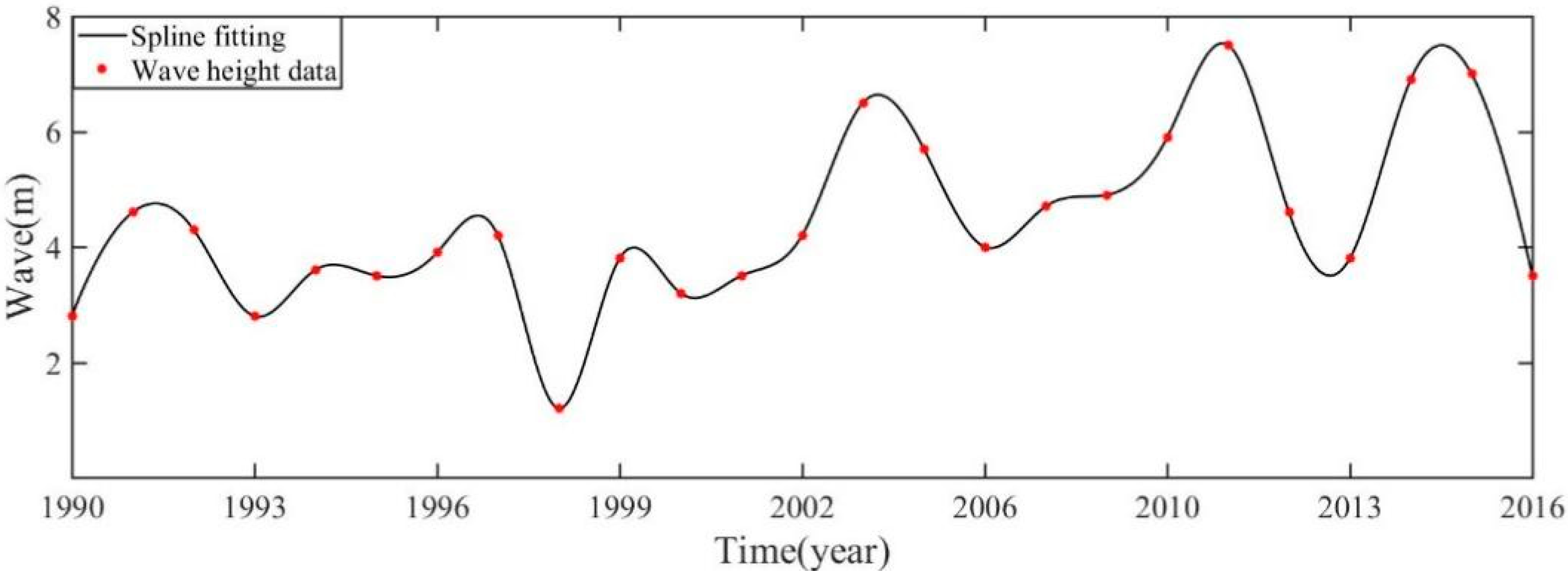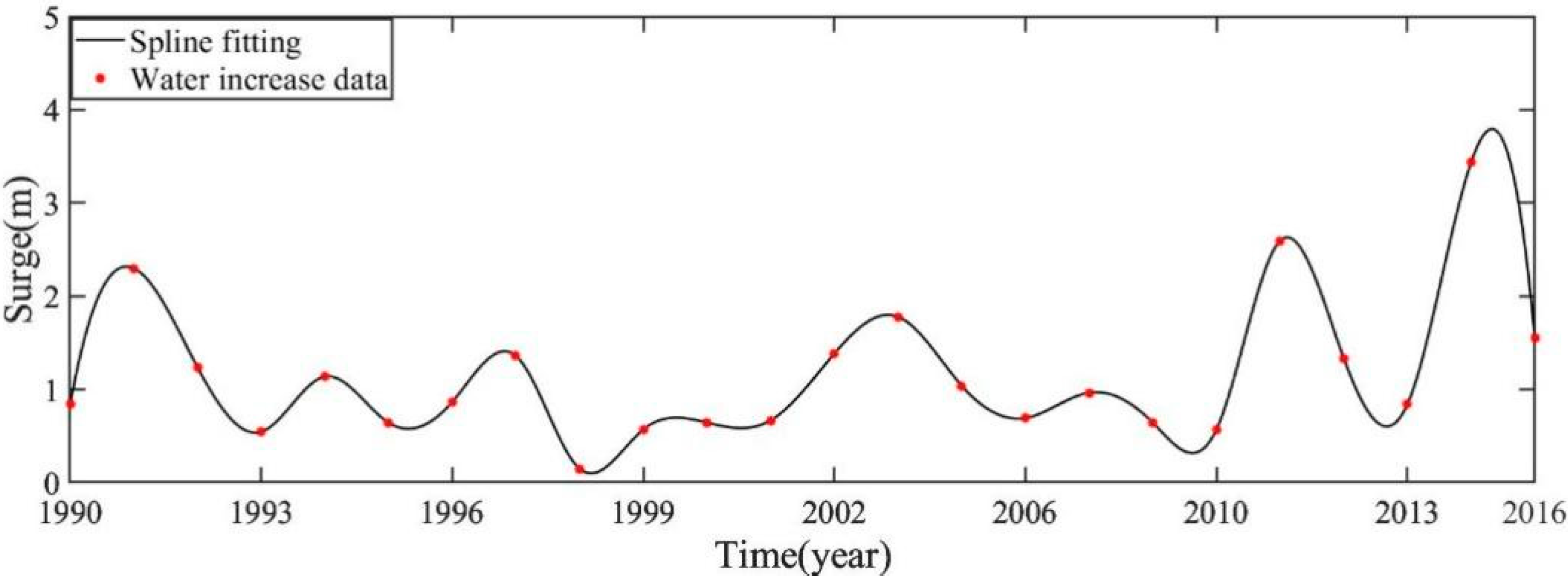That is, these data are sampled every 12 months ($\mathsf{\Delta }T=12$): Figure 3 and Figure 4 are the 25-year wave height and water increase data set sampling every 12 months from 1990 to 2016, respectively.

First, the samples of the wave height and water increase are examined. The K-S test results are listed for the Gumbel distribution, Weibull distribution, Pareto distribution, and Pearson-Ⅲ distribution of the wave height and water increase time series. The results showed that all four groups of sequences passed the K-S test, where $Dn$ is test value, $D_0$ is critical value, as shown in

Table 1. K-S test of the distribution models of wave height series ($\mathsf{\Delta }t=12$).

Distribution Model	Gumbel	Weibull	Pearson-Ⅲ	Pareto
Test value $Dn$	0.2089	0.1542	0.1138	0.2222
Critical value $D_0$ (0.05)	0.2641	0.2641	0.2641	0.2377
Compare	$Dn$< $D_0$	$Dn$< $D_0$	$Dn$< $D_0$	$Dn$< $D_0$
test result	accept	accept	accept	accept

and

Table 2. K-S test of the distribution model of increasing water series ($\mathsf{\Delta }t=12$).

Distribution Model	Gumbel	Weibull	Pearson-III	Pareto
Test value $Dn$	0.2354	0.1496	0.1224	0.1403
Critical value $D_0$ (0.05)	0.2641	0.2641	0.2641	0.2377
Compare	$Dn$ < $D_0$	$Dn$ < $D_0$	$Dn$ < $D_0$	$Dn$ < $D_0$
test result	accept	accept	accept	accept

.

Table 3. Comparison of fitting results of different probability density functions to wave height tail data.

	Gumbel		Weibull		EED-Ⅰ
Wave height(m)	20 years	16 years	20 years	16 years	20 years	16 years
8.0	0.0256	0.0357	0.0206	0.0343	0.0333	0.0443
8.5	0.0170	0.0243	0.0086	0.0157	0.0219	0.0245
9.0	0.0112	0.0165	0.0030	0.0061	0.0157	0.0157
9.5	0.0074	0.0111	0.0009	0.0020	0.0125	0.0128
10.0	0.0049	0.0075	0.0002	0.0006	0.0110	0.0121

and

Table 4. Comparison of fitting results of different probability density functions to water increase tail data.

	Gumbel		Weibull		EED-Ⅰ
Water increase(m)	20 years	16 years	20 years	16 years	20 years	16 years
2.00	0.1438	0.1701	0.1727	0.2028	0.1603	0.1816
2.25	0.0848	0.1064	0.0922	0.1212	0.0986	0.1152
2.50	0.0494	0.0655	0.0445	0.0670	0.0610	0.0730
2.75	0.0286	0.0400	0.0194	0.0343	0.0391	0.0473
3.00	0.0165	0.0243	0.0077	0.0163	0.0267	0.0320

show the specific probability density values when different distributions are fitted to the tail data. It can also be seen that, compared with the commonly used extreme value models, the EED-I model can better describe the tail characteristics of the data when fitting different marine environmental element data under different data ages. Taking the probability density values of different distributions corresponding to the wave height of 8.5 m in Table 3 for example, when the data age is 20 years, the probability density value of the EED-I distribution is 0.0125, which is 28.8% larger than the probability density value of the Gumbel distribution, and is 154.65% larger than the probability density value under the Weibull distribution; when the data age is 16 years, the probability density value of the EED-I distribution is 8.23% larger than the probability density value under the Gumbel, and 56.05% larger than the probability density value under the Weibull distribution.

In order to further verify the stability of the model, a period of time (1998–2016) in the wave height sequence was extracted, and the Gumbel and EED-I type distributions were used to calculate the design wave heights under different return periods, and compared with the entire time series, namely, the wave height data of Naozhou Station from 1990 to 2016. The design wave height and error calculated by different distribution models under different return periods are obtained, as shown in

Table 5. Design wave height and error of each model for different time periods.

	EED-Ⅰ			Gumbel
Return period (years)	25 years	17 years	error	25 years	17 years	error
10	6.3888	6.5505	2.53%	6.5913	6.8819	4.41%
20	7.0821	7.2788	2.78%	7.4786	7.8634	5.15%
50	7.9180	8.1581	3.03%	8.6210	9.1339	5.95%
100	8.5087	8.7802	3.20%	9.4780	10.0859	6.41%

. It can be seen from Table 5 that when the measured data years are reduced, the two distribution models will produce certain errors, and the longer the return period, the greater the error. However, the error of the EED-I distribution is much smaller than that of the traditional Gumbel distribution. Under the condition of a return period of 100 years, the error of the EED-I distribution is almost only half of that of the Gumbel distribution.

According to the wave height and water increase data of Naozhou Station from 1990 to 2016, the return levels of the wave height and water increase in different return periods under the EED-I type distribution are calculated, as shown in

Table 6. The return level of wave height and water increase in different return periods based on EED-I type distribution.

Return Period (Years)	Wave Height Return Level (m)	Water Increase Return Level (m)
10	6.5505	1.2745
20	7.2788	1.5810
50	8.1581	1.9802
100	8.7802	2.2785

.

According to the likelihood function and Gumbel–Pareto distribution, we obtained the respective parameter estimates for marginal distribution of the probability model; the results are shown in

Table 7. Marginal distribution parameters of wave height and water increase ($\mathsf{\Delta }t=12$).

		Wave Height	Water Increase
Parameters for marginal distribution	Parameter $\mu$	5.1952	1.5197
	Confidence interval	[4.5784,5.8121]	[1.1543,1.8851]
	Parameter $\xi$	1.4797	0.8736
	Confidence interval	[1.1142,1.9651]	[0.6750,1.1305]

.

According to Table 6, for the once-in-a-hundred-year value of $\mathsf{\Delta }T=12$ month series, wave height is 8.78 m and the water increase is 2.28 m. The corresponding combination of once-in-a-hundred-year calculated by using the new stochastic compound distribution model are 8.74 m for the effective wave height, and 1.52 m for the water increase.

The design of the deck elevation should consider many factors, the most important of which are the astronomical tide, storm surge and wave height that constitute the elevation of the water body. Other uncertain factors such as the subsidence of the platform and the seabed are generally not specifically studied; therefore, the deck elevation is generally often provided with sufficient spacing above the design wave crest. In addition, consideration should be given to providing an air gap between the height of the wave crest and the deck, generally 1.5 m, for waves larger than the design wave to pass.

Astronomical tides have deterministic and periodic laws. The trend value of the tide level change can be determined by the deterministic tidal force; the fluctuation value of the tide level change is affected by its random hydrological and geographic factors. Therefore, if the small random fluctuations of the tide level are ignored, the astronomical tide can be regarded as a certain natural phenomenon with a long period of 18.61 years. In this paper, the astronomical tidal height datum is located at 2.24 m below the mean sea level. We use the highest annual extreme astronomical tidal level at Naozhou Station from 2000 to 2018 at 2.02 m.

To determine the design value of the maximum wave height, the “Standards for Classification and Construction of Offshore Mobile Drilling Ships” of the Ship Inspection Bureau of the People’s Republic of China and the “Guidelines for the Design of Marine Steel Structures” of Japan are used and these stipulate that the maximum design wave height is $H_{max}=\mathit{min}\left\{2H_{1/3},H_b\right\}$

In which, $H_b$ is the breaking critical wave height and $H_{1/3}$ is the once-in-a-hundred-year wave height. The effective wave height calculated by the stochastic compound distribution is used here, which is 8.74 m.

According to China’s “Seaport Engineering Standards”, when the submarine slope $i<1140$, the ratio of the breaking wave height and the water depth of the wave can be determined according to

Table 8. Maximum ratio of breaking wave height to breaking water depth on gentle slopes.

$i$	≤1/1000	1/500	1/400	1/300	1/200
${\left(H_b/d_b\right)}_{max}$	0.60	0.60	0.61	0.63	0.69

, so that the maximum wave height design value $H_{max}$ can be obtained.

Assuming the offshore platform has a water depth of 35 m and a slope ratio of 1/200. Therefore, the breaking wave height is =24.15 m, so the maximum wave height design value is taken as $H_{max}=\mathit{min}\left\{2H_{1/3},H_b\right\}=2H_{1/3}=17.48 \mathrm{m}$

So far, the design values of each environmental element are obtained: the maximum wave crest is 8.74 m (0.5 times the maximum design wave height); the water increase is 1.52 m; the astronomical tide is 2.02 m; the air gap is 1.5 m. Therefore, the design value of the deck elevation calculated by the stochastic compound distribution model is 13.78 m. In the once-in-a-hundred-year time, the univariate EED-Ⅰ distribution calculates the wave height and the return period of the increase in water. The comparison between the simple superposition method and the calculation result of the new model is shown in

Table 9. Comparison of calculation results of univariate superposition and stochastic compound distribution ($\mathsf{\Delta }t=12)$.

	${\mathit{A}}_1$	${\mathit{A}}_2$	Astronomical Tide /m	Air Gap /m	Platform Height/m
Univariate superposition	8.78	2.28	2.02	1.50	14.58
Stochastic compound distribution	8.74	1.52	2.02	1.50	13.78

, where $A_1$ is Maximum Peak Height Once in a Hundred Years/m, $A_2$ is Water Increase Once in a Hundred Years/m.

It can be seen from Table 9 that the stochastic compound distribution takes into account the correlation between wave height and water increase, and its calculation result is slightly lower than that of univariate superposition, which improves the problem of high design value caused by simple superposition of univariate, and thus can reduce engineering cost with certain practical significance.

4. Conclusions

In this paper, the wave height and water increase are regarded as stochastic processes, and on this basis, an EED-I type distribution based on stochastic processes and extreme value expansion is derived and treated as a univariate marginal distribution. Moreover, with the Gumbel–Copula structure function applied as the connection, we are able to establish a new stochastic compound distribution model. The measured hydrological data of the flood period from 1990 to 2016 at Naozhou Station are used as data to analyze the wave height, water increase, and the joint return period of the two, and based on which the calculation of the bottom deck height in the area can be performed with the following conclusions:

• Based on stochastic process and extreme value expansion, the EED-I type distribution can better describe the tail characteristics of wave height and water increase, and it has obvious advantages in comparison with traditional extreme value distribution.
• Based on stochastic process and extreme value expansion, the EED-I type distribution has good stability under the condition of less measured data. When calculating the once-in-a-hundred-year return level, the error caused by the reduction of measured data is almost only half of the traditional Gumbel distribution, that is, the EED-I type distribution can be applied to the calculation of the return level in sea areas with less measured data.
• The stochastic compound distribution model takes into account the interaction of wave height and water increase, and improves the issues of high design value caused by simple superposition of univariate return level. It can calculate the bottom deck elevation more accurately under the premise of ensuring the safety of offshore platforms while at the same time save its engineering cost. Therefore, it is with certain practical value.