
Exploring the Drivers of Sentinel-2-Derived Crop Phenology: The Joint Role of Climate, Soil, and Land Use


Abstract
1. Introduction
2. Materials and Methods
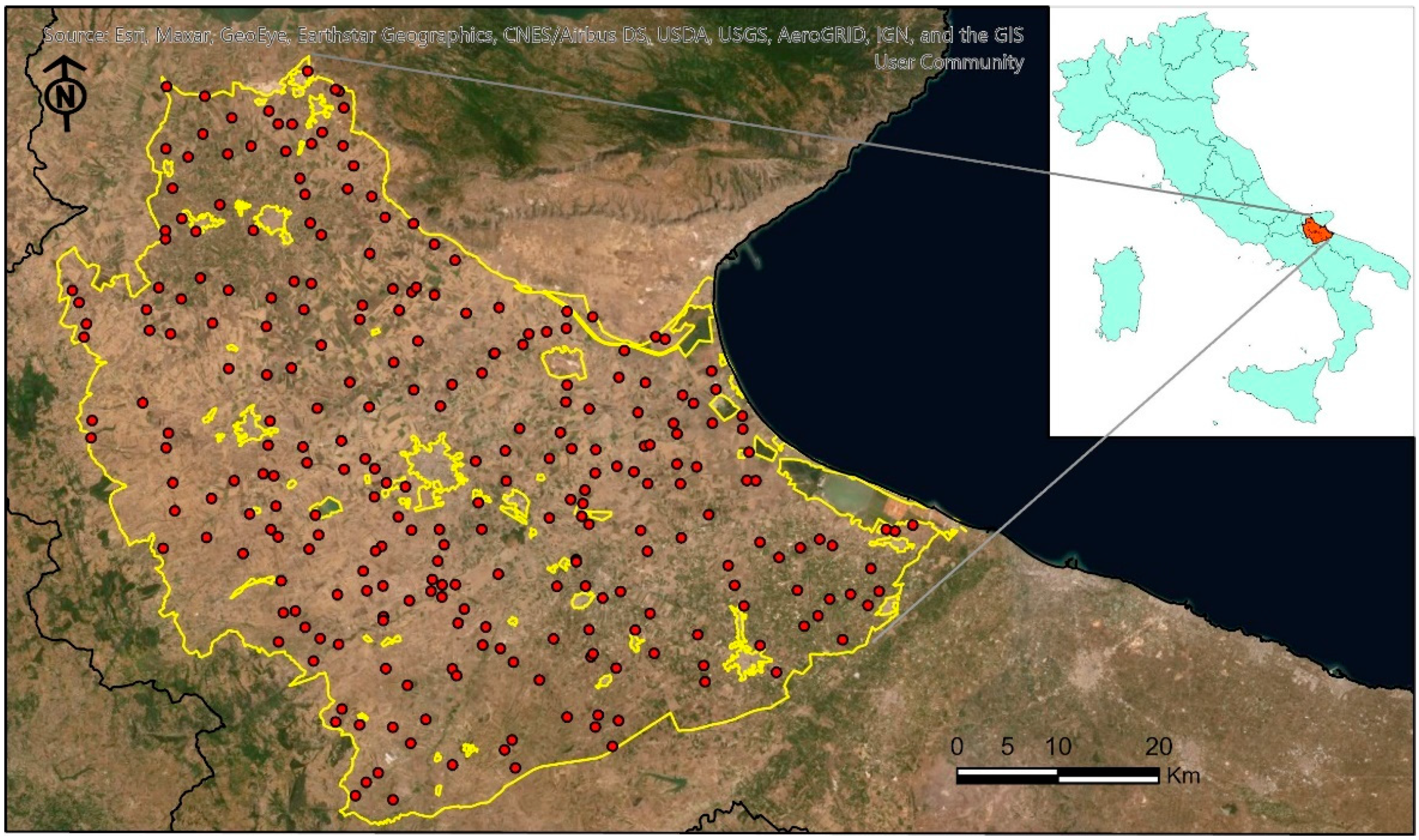
2.1. Study Area
2.2. Environmental Data
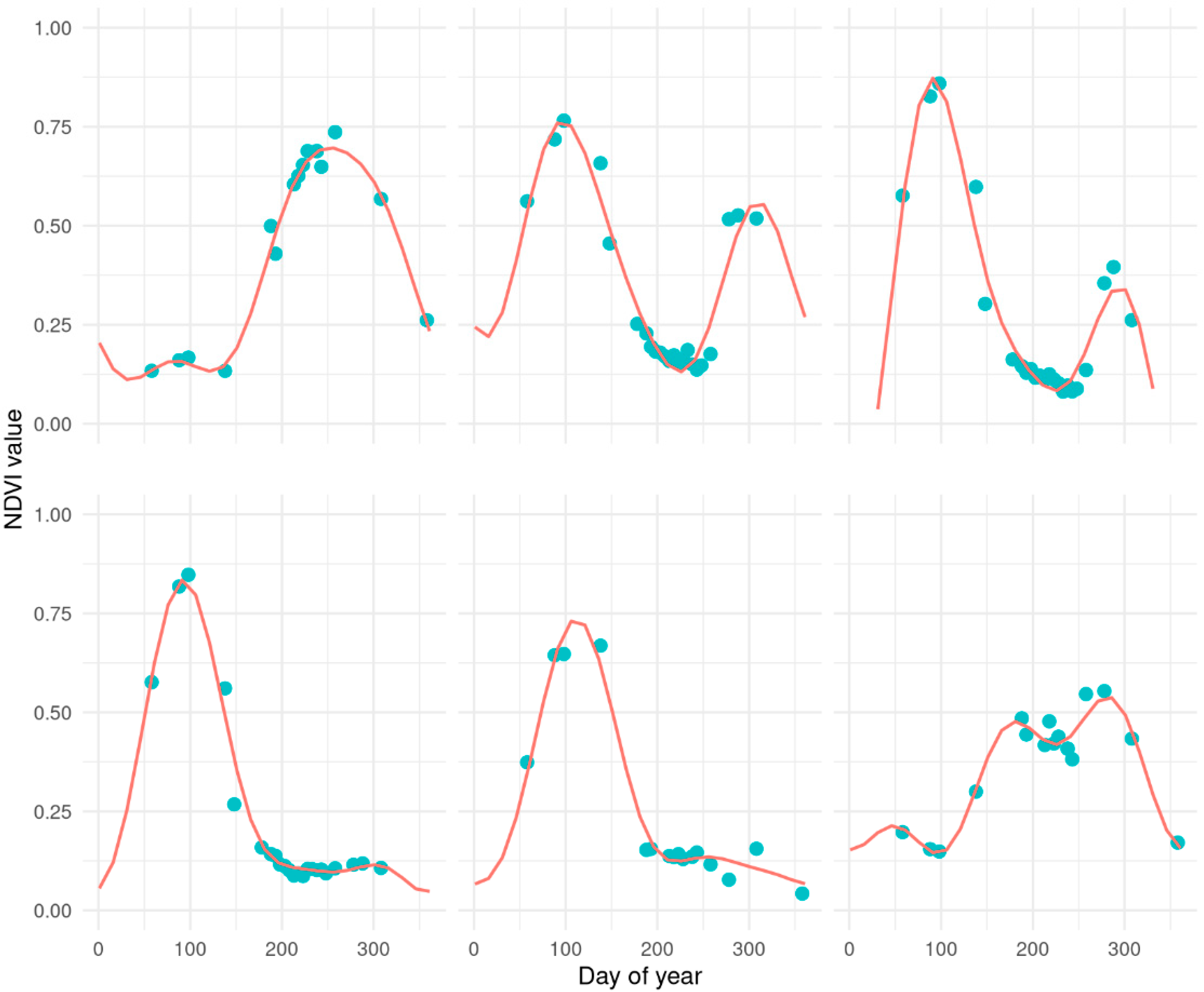
2.3. Satellite Data
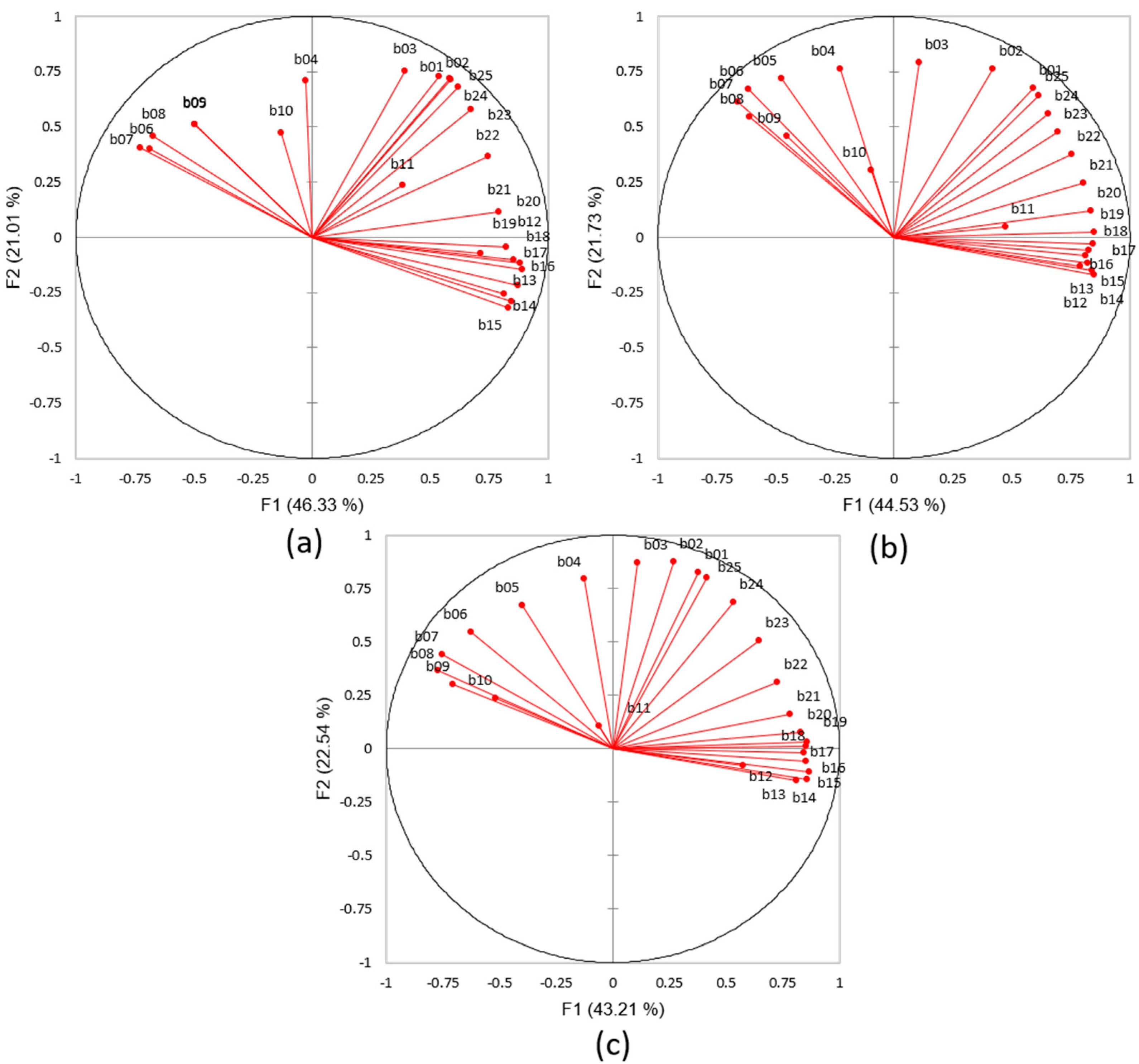
2.4. Methodology
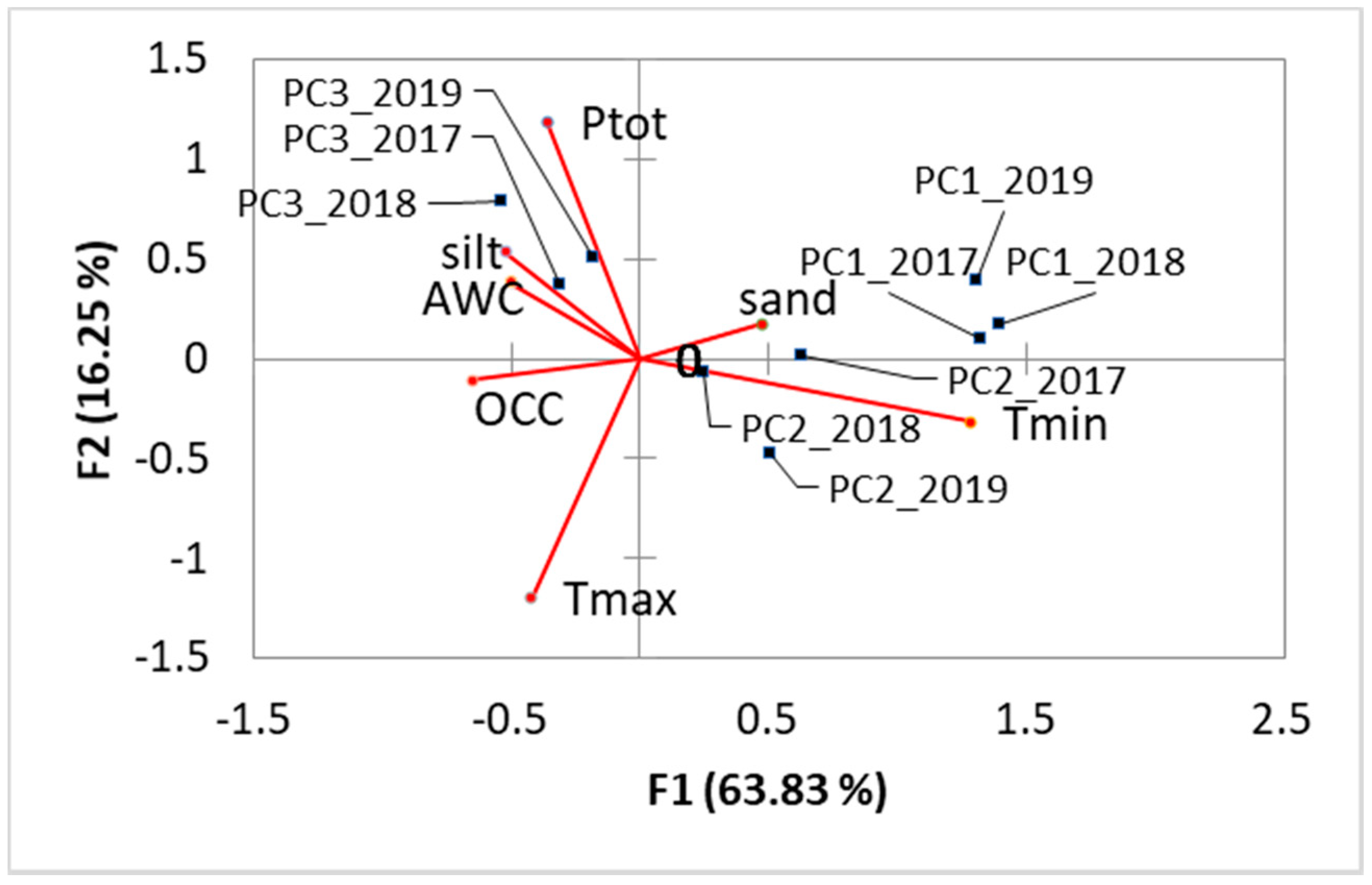
3. Results
4. Discussion
5. Conclusions
Author Contributions
Funding
Institutional Review Board Statement
Informed Consent Statement
Data Availability Statement
Conflicts of Interest
References
- Lieth, H. (Ed.) Purposes of a Phenology Book. In Phenology and Seasonality Modeling. Ecological Studies (Analysis and Synthesis); Springer: Berlin/Heidelberg, Germany, 1974; Volume 8, pp. 3–19. [Google Scholar]
- Ruml, M.; Vulic, T. Importance of phenological observations and predictions in agriculture. J. Agric. Sci. Belgrade 2005, 50, 217–225. [Google Scholar] [CrossRef]
- Bajocco, S.; Ferrara, C.; Alivernini, A.; Bascietto, M.; Ricotta, C. Remotely-sensed phenology of Italian forests: Ghueoing beyond the species. Int. J. Appl. Earth Obs. Geoinf. 2019, 74, 314–321. [Google Scholar] [CrossRef]
- Huang, X.; Liu, J.; Zhu, W.; Atzberger, C. The Optimal Threshold and Vegetation Index Time Series for Retrieving Crop Phenology Based on a Modified Dynamic Threshold Method. Remote Sens. 2019, 11, 2725. [Google Scholar] [CrossRef]
- Desanker, G.; Dahlin, K.M.; Finley, A.O. Environmental controls on Landsat-derived phenoregions across an East African megatransect. Ecosphere 2020, 11, e03143. [Google Scholar] [CrossRef]
- Luo, Y.; Zhang, Z.; Chen, Y.; Li, Z.; Tao, F. ChinaCropPhen1km: A high-resolution crop phenological dataset for three staple crops in China during 2000–2015 based on leaf area index (LAI) products. Earth Syst. Sci. Data 2020, 12, 197–214. [Google Scholar] [CrossRef]
- Ogle, S.M.; Breidt, F.J.; Paustian, K. Agricultural management impacts on soil organic carbon storage under moist and dry climatic conditions of temperate and tropical regions. Biogeochemistry 2005, 72, 87–121. [Google Scholar] [CrossRef]
- Heupel, K.; Spengler, D.; Itzerott, S. A Progressive Crop-Type Classification Using Multitemporal Remote Sensing Data and Phenological Information. PFG J. Photogramm. Remote Sens. Geoinf. Sci. 2018, 86, 53–69. [Google Scholar] [CrossRef]
- Bégué, A.; Arvor, D.; Bellon, B.; Betbeder, J.; De Abelleyra, D.; Ferraz, R.P.D.; Lebourgeois, V.; Lelong, C.; Simões, M.; Verón, S.R. Remote Sensing and Cropping Practices: A Review. Remote Sens. 2018, 10, 99. [Google Scholar] [CrossRef]
- White, M.A.; Nemani, R.R. Real-time monitoring and short-term forecasting of land surface phenology. Remote Sens. Environ. 2006, 104, 43–49. [Google Scholar] [CrossRef]
- Atkinson, P.M.; Jeganathan, C.; Dash, J.; Atzberger, C. Inter-comparison of four models for smoothing satellite sensor time-series data to estimate vegetation phenology. Remote Sens. Environ. 2012, 123, 400–417. [Google Scholar] [CrossRef]
- Rouse, J.W., Jr.; Haas, R.H.; Schell, J.A.; Deering, D.W. Monitoring Vegetation Systems in the Great Plains with Erts. NASA Spec. Publ. 1974, 351, 309. [Google Scholar]
- Reed, B.C.; Brown, J.F.; Vanderzee, D.; Loveland, T.R.; Merchant, J.W.; Ohlen, D.O. Measuring phenological variability from satellite imagery. J. Veg. Sci. 1994, 5, 703–714. [Google Scholar] [CrossRef]
- Bellón, B.; Bégué, A.; Seen, D.L.; De Almeida, C.A.; Simões, M. A Remote Sensing Approach for Regional-Scale Mapping of Agricultural Land-Use Systems Based on NDVI Time Series. Remote Sens. 2017, 9, 600. [Google Scholar] [CrossRef]
- Liu, J.; Zhu, W.; Cui, X. A Shape-Matching Cropping Index (CI) Mapping Method to Determine Agricultural Cropland In-tensities in China Using MODIS Time-Series Data. Photogramm. Eng. Remote Sens. 2012, 78, 829–837. [Google Scholar] [CrossRef]
- Sakamoto, T.; Van Nguyen, N.; Ohno, H.; Ishitsuka, N.; Yokozawa, M. Spatio–temporal distribution of rice phenology and cropping systems in the Mekong Delta with special reference to the seasonal water flow of the Mekong and Bassac rivers. Remote Sens. Environ. 2006, 100, 1–16. [Google Scholar] [CrossRef]
- Lv, T.; Liu, C. Study on Extraction of Crop Information Using Time-Series MODIS Data in the Chao Phraya Basin of Thailand. Adv. Space Res. 2010, 45, 775–784. [Google Scholar]
- Wardlow, B.D.; Egbert, S.L.; Kastens, J.H. Analysis of time-series MODIS 250 m vegetation index data for crop classification in the U.S. Central Great Plains. Remote Sens. Environ. 2007, 108, 290–310. [Google Scholar] [CrossRef]
- Foerster, S.; Kaden, K.; Foerster, M.; Itzerott, S. Crop type mapping using spectral–temporal profiles and phenological information. Comput. Electron. Agric. 2012, 89, 30–40. [Google Scholar] [CrossRef]
- Seyednasrollah, B.; Young, A.M.; Li, X.; Milliman, T.; Ault, T.; Frolking, S.; Friedl, M.; Richardson, A.D. Sensitivity of Deciduous Forest Phenology to Environmental Drivers: Implications for Climate Change Impacts Across North America. Geophys. Res. Lett. 2020, 47, 47. [Google Scholar] [CrossRef]
- Dahlgren, J.P.; von Zeipel, H.; Ehrlén, J. Variation in Vegetative and Flowering Phenology in a Forest Herb Caused by Envi-ronmental Heterogeneity. Am. J. Bot. 2007, 94, 1570–1576. [Google Scholar] [CrossRef]
- Pastor-Guzman, J.; Dash, J.; Atkinson, P.M. Remote sensing of mangrove forest phenology and its environmental drivers. Remote Sens. Environ. 2018, 205, 71–84. [Google Scholar] [CrossRef]
- Li, P.; Peng, C.; Wang, M.; Luo, Y.; Li, M.; Zhang, K.; Zhang, D.; Zhu, Q. Dynamics of vegetation autumn phenology and its response to multiple environmental factors from 1982 to 2012 on Qinghai-Tibetan Plateau in China. Sci. Total Environ. 2018, 637, 855–864. [Google Scholar] [CrossRef]
- Gao, F.; Zhang, X. Mapping Crop Phenology in Near Real-Time Using Satellite Remote Sensing: Challenges and Opportunities. J. Remote Sens. 2021, 2021, 8379391. [Google Scholar] [CrossRef]
- Liu, J.; Zhu, W.; Atzberger, C.; Zhao, A.; Pan, Y.; Huang, X. A Phenology-Based Method to Map Cropping Patterns under a Wheat-Maize Rotation Using Remotely Sensed Time-Series Data. Remote Sens. 2018, 10, 1203. [Google Scholar] [CrossRef]
- Wu, W.-B.; Yang, P.; Tang, H.-J.; Zhou, Q.-B.; Chen, Z.-X.; Shibasaki, R. Characterizing Spatial Patterns of Phenology in Cropland of China Based on Remotely Sensed Data. Agric. Sci. China 2010, 9, 101–112. [Google Scholar] [CrossRef]
- Van Oosterzee, P.; Dale, A.; Preece, N. Integrating agriculture and climate change mitigation at landscape scale: Implications from an Australian case study. Glob. Environ. Chang. 2014, 29, 306–317. [Google Scholar] [CrossRef]
- Balenzano, A.; Satalino, G.; Lovergine, F.P.; Rinaldi, M.; Iacobellis, V.; Mastronardi, N.; Mattia, F. On the use of temporal series of L- and X-band SAR data for soil moisture retrieval. Capitanata plain case study. Eur. J. Remote Sens. 2013, 46, 721–737. [Google Scholar] [CrossRef]
- ISTAT. 2021. Available online: http://dati.istat.it/Index.aspx?DataSetCode=DCSP_COLTIVAZIONI (accessed on 17 June 2021).
- FAO. Guidelines for Soil Description; FAO: Rome, Italy, 2006; p. 97. [Google Scholar]
- Bruand, A.; Fernandez, P.P.; Duval, O. Use of class pedotransfer functions based on texture and bulk density of clods to generate water retention curves. Soil Use Manag. 2003, 19, 232–242. [Google Scholar] [CrossRef]
- Fick, S.E.; Hijmans, R.J. WorldClim 2: New 1-km spatial resolution climate surfaces for global land areas. Int. J. Climatol. 2017, 37, 4302–4315. [Google Scholar] [CrossRef]
- ISPRA. TERRITORIO Processi e Trasformazioni in Italia; ISPRA: Palermo, Italy, 2018; Rapporti 296/2018; ISBN 9788844809218. [Google Scholar]
- Gorelick, N.; Hancher, M.; Dixon, M.; Ilyushchenko, S.; Thau, D.; Moore, R. Google Earth Engine: Planetary-scale geospatial analysis for everyone. Remote Sens. Environ. 2017, 202, 18–27. [Google Scholar] [CrossRef]
- Bascietto, M.; Sperandio, G.; Bajocco, S. Efficient Estimation of Biomass from Residual Agroforestry. IJGI 2020, 9, 21. [Google Scholar] [CrossRef]
- Lasaponara, R. On the use of principal component analysis (PCA) for evaluating interannual vegetation anomalies from SPOT/VEGETATION NDVI temporal series. Ecol. Model. 2006, 194, 429–434. [Google Scholar] [CrossRef]
- Bajocco, S.; Rosati, L.; Ricotta, C. Knowing fire incidence through fuel phenology: A remotely sensed approach. Ecol. Model. 2010, 221, 59–66. [Google Scholar] [CrossRef]
- Teil, H. Correspondence factor analysis: An outline of its method. Math. Geol. 1975, 7, 3–12. [Google Scholar] [CrossRef]
- Addinsoft, A. XLSTAT Statistical and Data Analysis Solution; Addinsoft Inc.: Long Island, NY, USA, 2019. [Google Scholar]
- Araya, S.; Ostendorf, B.; Lyle, G.; Lewis, M. Remote Sensing Derived Phenological Metrics to Assess the Spatio-Temporal Growth Variability in Cropping Fields. Adv. Remote Sens. 2017, 6, 212–228. [Google Scholar] [CrossRef]
- Skuras, D.; Psaltopoulos, D.; Meybeck, A.; Lankoski, J.; Redfern, S.; Azzu, N.; Gitz, V. A Broad Overview of the Main Problems Derived from Climate Change that Will Affect Agricultural Production in the Mediterranean Area; FAO: Rome, Italy, 2012; p. 217. [Google Scholar]
- Meng, S.; Zhong, Y.; Luo, C.; Hu, X.; Wang, X.; Huang, S. Optimal Temporal Window Selection for Winter Wheat and Rapeseed Mapping with Sentinel-2 Images: A Case Study of Zhongxiang in China. Remote Sens. 2020, 12, 226. [Google Scholar] [CrossRef]
- Abuzar, M.; Rampant, P.; Fisher, P. Measuring Spatial Variability of Crops and Soils at Sub-Paddock Scale Using Remote Sensing Technologies. In Proceedings of the International Geoscience and Remote Sensing Symposium, Anchorage, AK, USA, 20–24 September 2004; Volume 3, pp. 1633–1636. [Google Scholar]
- Vanino, S.; Nino, P.; De Michele, C.; Bolognesi, S.F.; D’Urso, G.; Di Bene, C.; Pennelli, B.; Vuolo, F.; Farina, R.; Pulighe, G.; et al. Capability of Sentinel-2 data for estimating maximum evapotranspiration and irrigation requirements for tomato crop in Central Italy. Remote Sens. Environ. 2018, 215, 452–470. [Google Scholar] [CrossRef]
- Maynard, J.J.; Levi, M.R. Hyper-temporal remote sensing for digital soil mapping: Characterizing soil-vegetation response to climatic variability. Geoderma 2017, 285, 94–109. [Google Scholar] [CrossRef]


| Sand (%) | Silt (%) | OCC (Unitless) | AWC (Unitless) | |
|---|---|---|---|---|
| Min | 0.5 | 0.5 | 0.14 | 59.07 |
| Max | 96.5 | 80 | 4.5 | 219.14 |
| Mean | 28.8 | 35.43 | 1.28 | 140.70 |
| LU Code | Description | Surface (ha) |
|---|---|---|
| 211 | Non irrigated arable land | 70,915 |
| 212 | Permanently irrigated lands | 181,107 |
| 221 | Vineyards | 28,563 |
| 223 | Olive groves | 28,858 |
| Temporal Bands | Date | DOY | Temporal Bands | Date | DOY |
|---|---|---|---|---|---|
| b01 | 1-Jan | 1 | b14 | 15-Jul | 196 |
| b02 | 16-Jan | 16 | b15 | 30-Jul | 211 |
| b03 | 31-Jan | 31 | b16 | 14-Aug | 226 |
| b04 | 15-Feb | 46 | b17 | 29-Aug | 241 |
| b05 | 2-Mar | 61 | b18 | 13-Sep | 256 |
| b06 | 17-Mar | 76 | b19 | 28-Sep | 271 |
| b07 | 1-Apr | 91 | b20 | 13-Oct | 286 |
| b08 | 16-Apr | 106 | b21 | 28-Oct | 301 |
| b09 | 1-May | 121 | b22 | 12-Nov | 316 |
| b10 | 16-May | 136 | b23 | 27-Nov | 331 |
| b11 | 31-May | 151 | b24 | 12-Dec | 346 |
| b12 | 15-Jun | 166 | b25 | 27-Dec | 361 |
| b13 | 30-Jun | 181 |
Publisher’s Note: MDPI stays neutral with regard to jurisdictional claims in published maps and institutional affiliations. |
© 2021 by the authors. Licensee MDPI, Basel, Switzerland. This article is an open access article distributed under the terms and conditions of the Creative Commons Attribution (CC BY) license (https://creativecommons.org/licenses/by/4.0/).
Share and Cite
Bajocco, S.; Vanino, S.; Bascietto, M.; Napoli, R. Exploring the Drivers of Sentinel-2-Derived Crop Phenology: The Joint Role of Climate, Soil, and Land Use. Land 2021, 10, 656. https://doi.org/10.3390/land10060656
Bajocco S, Vanino S, Bascietto M, Napoli R. Exploring the Drivers of Sentinel-2-Derived Crop Phenology: The Joint Role of Climate, Soil, and Land Use. Land. 2021; 10(6):656. https://doi.org/10.3390/land10060656
Chicago/Turabian StyleBajocco, Sofia, Silvia Vanino, Marco Bascietto, and Rosario Napoli. 2021. "Exploring the Drivers of Sentinel-2-Derived Crop Phenology: The Joint Role of Climate, Soil, and Land Use" Land 10, no. 6: 656. https://doi.org/10.3390/land10060656
APA StyleBajocco, S., Vanino, S., Bascietto, M., & Napoli, R. (2021). Exploring the Drivers of Sentinel-2-Derived Crop Phenology: The Joint Role of Climate, Soil, and Land Use. Land, 10(6), 656. https://doi.org/10.3390/land10060656