
Assessment of Spatiotemporal Peak Shift of Intra-Urban Transportation Taking a Case in Bangkok, Thailand


Abstract
1. Introduction
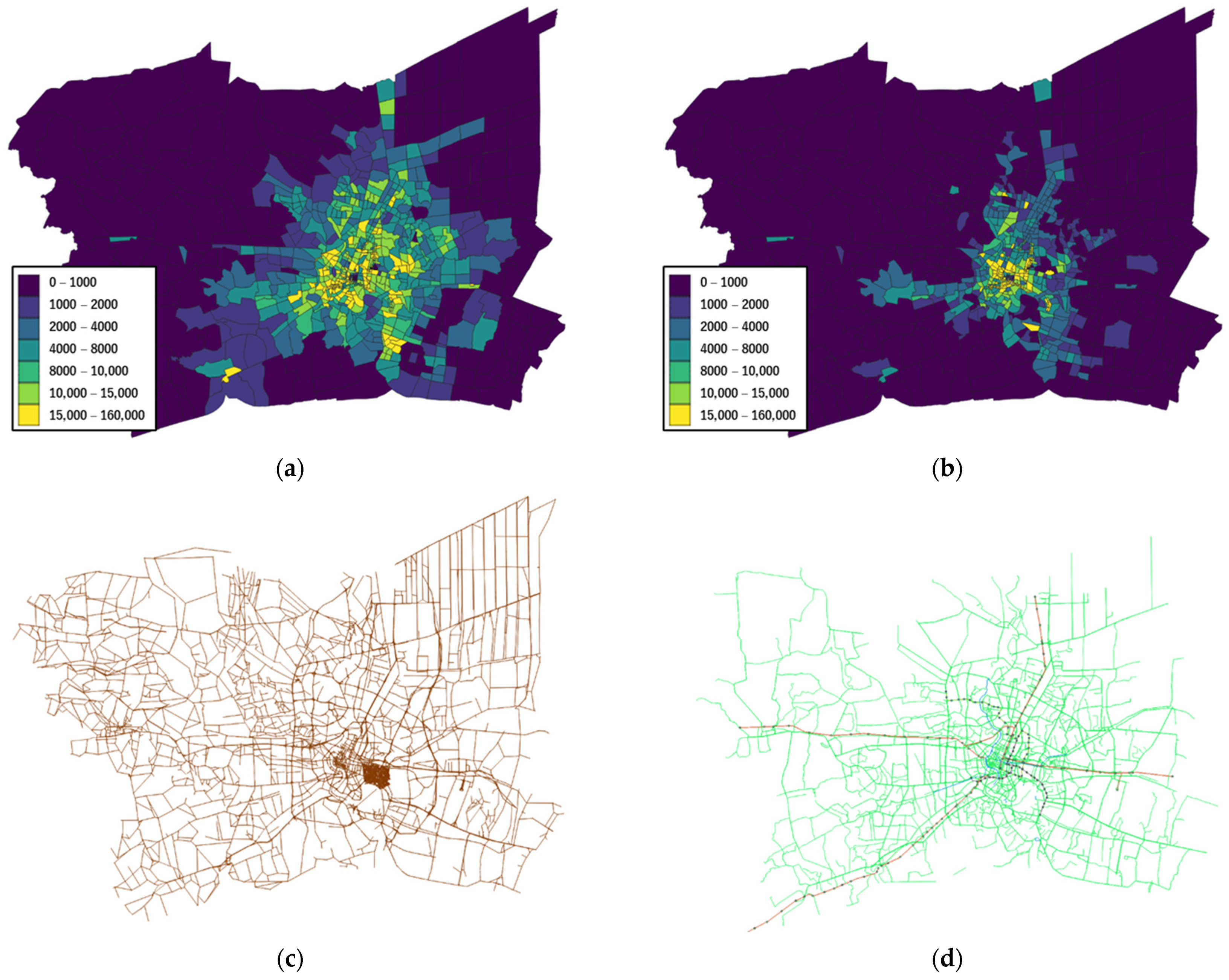
2. Data
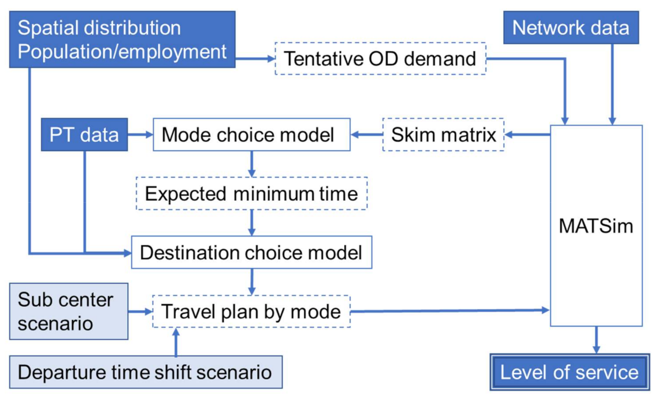
3. Method
4. Scenarios for Transport Policy Measures
5. Results
5.1. Validation
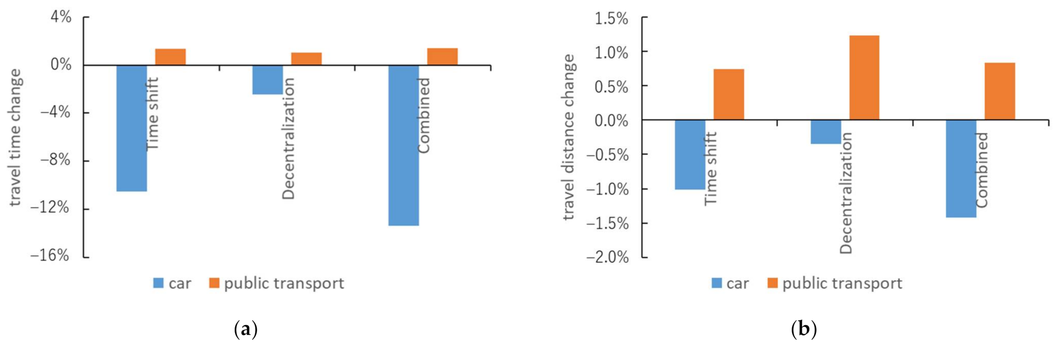
5.2. Effect of Policy Scenarios
6. Discussion and Conclusions
Author Contributions
Funding
Institutional Review Board Statement
Informed Consent Statement
Acknowledgments
Conflicts of Interest
References
- IEA. Energy Technology Perspectives; IEA: Paris, France, 2017. [Google Scholar]
- Dulal, H.B. Making cities resilient to climate change: Identifying “win–win” interventions. Local Environ. 2016, 22, 106–125. [Google Scholar] [CrossRef]
- Kii, M.; Nakanishi, H.; Nakamura, K.; Doi, K. Transportation and spatial development: An overview and a future direction. Transp. Policy 2016, 49, 148–158. [Google Scholar] [CrossRef]
- Ahmad, S.; de Oliveira, J.A.P. Determinants of urban mobility in India: Lessons for promoting sustainable and inclusive urban transportation in developing countries. Transp. Policy 2016, 50, 106–114. [Google Scholar] [CrossRef]
- Capurso, M.; Hess, S.; Dekker, T. Modelling the role of consideration of alternatives in mode choice: An application on the Rome-Milan corridor. Transp. Res. Part A Policy Pract. 2019, 129, 170–184. [Google Scholar] [CrossRef]
- Gao, Y.; Newman, P. Beijing’s Peak Car Transition: Hope for Emerging Cities in the 1.5 °C Agenda. Urban Plan. 2018, 3, 82–93. [Google Scholar] [CrossRef]
- Heinen, E.; Harshfield, A.; Panter, J.; Mackett, R.; Ogilvie, D. Does exposure to new transport infrastructure result in modal shifts? Patterns of change in commute mode choices in a four-year quasi-experimental cohort study. J. Transp. Health 2017, 6, 396–410. [Google Scholar] [CrossRef] [PubMed]
- Christiansen, P.; Engebretsen, Ø.; Fearnley, N.; Hanssen, J.U. Parking facilities and the built environment: Impacts on travel behaviour. Transp. Res. Part A Policy Pract. 2017, 95, 198–206. [Google Scholar] [CrossRef]
- Lehner, M.; Mont, O.; Heiskanen, E. Nudging—A promising tool for sustainable consumption behaviour? J. Clean. Prod. 2016, 134, 166–177. [Google Scholar] [CrossRef]
- Dieleman, F.; Wegener, M. Compact city and urban sprawl. Built Environ. 2004, 30, 308–323. [Google Scholar] [CrossRef]
- Brueckner, J.K. Urban sprawl: Diagnosis and remedies. Int. Reg. Sci. Rev. 2000, 23, 160–171. [Google Scholar] [CrossRef]
- Otero, I.; Nieuwenhuijsen, M.J.; Rojas-Rueda, D. Health impacts of bike sharing systems in Europe. Environ. Int. 2018, 115, 387–394. [Google Scholar] [CrossRef]
- Ricci, M. Bike sharing: A review of evidence on impacts and processes of implementation and operation. Res. Transp. Bus. Manag. 2015, 15, 28–38. [Google Scholar] [CrossRef]
- Toole, J.; Colak, S.; Sturt, B.; Alexander, L.; Evsukoff, A.; González, M. The path most traveled: Travel demand estimation using big data resources. Transp. Res. Part C Emerg. Technol. 2015, 58, 162–177. [Google Scholar] [CrossRef]
- Anda, C.; Fourie, P.; Erath, A. Transport Modelling in the Age of Big Data. Int. J. Urban Sci. 2016, 21, 19–42. [Google Scholar] [CrossRef]
- Milne, D.; Watling, D. Big data and understanding change in the context of planning transport systems. J. Transp. Geogr. 2019, 76, 235–244. [Google Scholar] [CrossRef]
- Jittrapirom, P.; Marchau, V.; van der Heijden, R.; Meurs, H. Future implementation of mobility as a service (MaaS): Results of an international Delphi study. Travel Behav. Soc. 2020, 21, 281–294. [Google Scholar] [CrossRef]
- Jittrapirom, P.; Caiati, V.; Feneri, A.-M.; Ebrahimigharehbaghi, S.; González, M.J.A.; Narayan, J. Mobility as a Service: A Critical Review of Definitions, Assessments of Schemes, and Key Challenges. Urban Plan. 2017, 2, 13–25. [Google Scholar] [CrossRef]
- Noy, K.; Givoni, M. Is ‘Smart Mobility’ Sustainable? Examining the Views and Beliefs of Transport’s Technological Entrepreneurs. Sustainability 2018, 10, 422. [Google Scholar] [CrossRef]
- Gössling, S. Tourism, information technologies and sustainability: An exploratory review. J. Sustain. Tour. 2017, 25, 1024–1041. [Google Scholar] [CrossRef]
- Tafidis, P.; Macedo, E.; Coelho, M.C.; Niculescu, M.C.; Voicu, A.; Barbu, C.; Jianu, N.; Pocostales, F.J.M.; Laranjeira, C.M.; Bandeira, J. Exploring the impact of ICT on urban mobility in heterogenic regions. Transp. Res. Procedia 2017, 27, 309–316. [Google Scholar] [CrossRef]
- Newman, P.; Hargroves, K.; Davies-Slate, S.; Conley, D.; Verschuer, M.; Mouritz, M.; Yangka, D. The Trackless Tram: Is It the Transit and City Shaping Catalyst We Have Been Waiting for? J. Transp. Technol. 2019, 9, 31–55. [Google Scholar] [CrossRef]
- Wethyavivorn, P.; Sukwattanakorn, N. Problems and barriers affecting sustainable commuting: Case study of people’s daily commute to Kasetsart University, Bangkok, Thailand. IOP Conf. Ser. Earth Environ. Sci. 2019, 329, 31–55. [Google Scholar] [CrossRef]
- Peungnumsai, A.; Miyazaki, H.; Witayangkurn, A.; Kim, S.M. A Grid-Based Spatial Analysis for Detecting Supply–Demand Gaps of Public Transports: A Case Study of the Bangkok Metropolitan Region. Sustainability 2020, 12, 382. [Google Scholar] [CrossRef]
- Ito, K.; Nakamura, K.; Kato, H.; Hayashi, Y. Influence of Urban Railway Development Timing on Long-term Car Ownership Growth in Asian Developing Mega-cities. J. East. Asia Soc. Transp. Stud. 2013, 10, 1076–1085. [Google Scholar] [CrossRef]
- Prasertsubpakij, D.; Nitivattananon, V. Evaluating accessibility to Bangkok Metro Systems using multi-dimensional criteria across user groups. IATSS Res. 2012, 36, 56–65. [Google Scholar] [CrossRef]
- Witchayaphong, P.; Pravinvongvuth, S.; Kanitpong, K.; Sano, K.; Horpibulsuk, S. Influential Factors Affecting Travelers’ Mode Choice Behavior on Mass Transit in Bangkok, Thailand. Sustainability 2020, 12, 9522. [Google Scholar] [CrossRef]
- Dissanayake, D.; Morikawa, T. Impact assessment of satellite centre-based telecommuting on travel and air quality in developing countries by exploring the link between travel behaviour and urban form. Transp. Res. Part A Policy Pract. 2008, 42, 883–894. [Google Scholar] [CrossRef]
- Mitchell, R.B.; Rapkin, C. Urban Traffic; Columbia University Press: New York, NY, USA, 1954. [Google Scholar]
- Bazzan, A.L.C.; Klügl, F. A review on agent-based technology for traffic and transportation. Knowl. Eng. Rev. 2013, 29, 375–403. [Google Scholar] [CrossRef]
- Smith, D.M.; Clarke, G.P.; Harland, K. Improving the Synthetic Data Generation Process in Spatial Microsimulation Models. Environ. Plan. A Econ. Space 2009, 41, 1251–1268. [Google Scholar] [CrossRef]
- Patterson, Z.; Kryvobokov, M.; Marchal, F.; Bierlaire, M. Disaggregate models with aggregate data: Two UrbanSim applications. J. Transp. Land Use 2010, 3. [Google Scholar] [CrossRef]
- Horni, A.; Nagel, K.; Axhausen, K. (Eds.) Multi-Agent Transport Simulation MATSim; Ubiquity Press: London, UK, 2016. [Google Scholar]
- Marchal, F. A Trip Generation Method for Time-Dependent Large-Scale Simulations of Transport and Land-Use. Netw. Spat. Econ. 2005, 5, 179–192. [Google Scholar] [CrossRef]
- Duleba, S.; Moslem, S.; Esztergár-Kiss, D. Estimating commuting modal split by using the Best-Worst Method. Eur. Transp. Res. Rev. 2021, 13, 1–12. [Google Scholar] [CrossRef]
- Altieri, M.; Silva, C.; Terabe, S. Give public transit a chance: A comparative analysis of competitive travel time in public transit modal share. J. Transp. Geogr. 2020, 87, 102817. [Google Scholar] [CrossRef]
- Achariyaviriya, W.; Hayashi, Y.; Takeshita, H.; Kii, M.; Vichiensan, V.; Theeramunkong, T. Can Space–Time Shifting of Activities and Travels Mitigate Hyper-Congestion in an Emerging Megacity, Bangkok? Effects on Quality of Life and CO2 Emission. Sustainability 2021, 13, 6547. [Google Scholar] [CrossRef]
- Llorca, C.; Moeckel, R. Effects of scaling down the population for agent-based traffic simulations. Procedia Comput. Sci. 2019, 151, 782–787. [Google Scholar] [CrossRef]
- Kii, M. Projecting future populations of urban agglomerations around the world and through the 21st century. NPJ Urban Sustain. 2021, 1, 1–12. [Google Scholar] [CrossRef]
- Kii, M.; Moeckel, R.; Thill, J.-C. Land use, transport, and environment interactions: WCTR 2016 contributions and future research directions. Comput. Environ. Urban Syst. 2019, 77. [Google Scholar] [CrossRef]
- Kii, M.; Akimoto, K.; Doi, K. Measuring the impact of urban policies on transportation energy saving using a land use-transport model. IATSS Res. 2014, 37, 98–109. [Google Scholar] [CrossRef]
- Kii, M. Reductions in CO2 Emissions from Passenger Cars under Demography and Technology Scenarios in Japan by 2050. Sustainability 2020, 12, 6919. [Google Scholar] [CrossRef]
- Moeckel, R. Constraints in household relocation: Modeling land-use/transport interactions that respect time and monetary budgets. J. Transp. Land Use 2016, 10. [Google Scholar] [CrossRef]
- Llorca, C.; Silva, C.; Kuehnel, N.; Moreno, A.; Zhang, Q.; Kii, M.; Moeckel, R. Integration of Land Use and Transport to Reach Sustainable Development Goals: Will Radical Scenarios Actually Get Us There? Sustainability 2020, 12, 9795. [Google Scholar] [CrossRef]


| Name | Provider | Description |
|---|---|---|
| Household Travel Survey (HTS) | The Office of Transport and Traffic Policy and planning (OTP) | Travel survey data of 18,833 households accounting for 38,054 people conducted in 2017 |
| Traffic analysis zone (TAZ) | 846 zones | |
| Public transport | GTFS data for rail lines, bus routes, and ferry (2019) | |
| Population and household | National Statistical Office | Number of population and household (2010) |
| Employment | Number of employment (2014) | |
| Population | MapFan DB Data Model | Population estimates of subdistrict by age and gender (2017) |
| Road network | Road link attributes (2018) |
| Age Class | Male | Female | |||||
|---|---|---|---|---|---|---|---|
| Transit Dummy | Walk Dummy | Time Coefficient | Transit Dummy | Walk Dummy | Time Coefficient | ||
| <10 | parameters | 0.033 | −2.279 | −0.002 | −0.021 | −2.086 | 0.002 |
| t-value | 0.140 | −5.933 | −0.616 | −0.116 | −7.025 | 0.820 | |
| p-value | 0.532 | 0.409 | |||||
| McFadden R2 | 0.001 | 0.001 | |||||
| 10–19 | parameters | 0.583 | −1.600 | −0.007 | 1.193 | −1.067 | −0.008 |
| t-value | 7.316 | −12.589 | −5.498 | 15.931 | −9.248 | −6.555 | |
| p-value | 0.000 | 0.000 | |||||
| McFadden R2 | 0.012 | 0.014 | |||||
| 20–29 | parameters | −0.168 | −2.216 | −0.009 | 0.571 | −1.508 | −0.010 |
| t-value | −3.869 | −29.719 | −11.188 | 16.229 | −27.096 | −15.663 | |
| p-value | 0.000 | 0.000 | |||||
| McFadden R2 | 0.014 | 0.019 | |||||
| 30–39 | parameters | −0.864 | −2.994 | −0.010 | −0.442 | −2.624 | −0.008 |
| t-value | −17.412 | −31.305 | −9.589 | −10.450 | −32.974 | −9.566 | |
| p-value | 0.000 | 0.000 | |||||
| McFadden R2 | 0.013 | 0.010 | |||||
| 40–49 | parameters | −1.250 | −3.303 | −0.011 | −0.598 | −2.427 | −0.006 |
| t-value | −16.161 | −23.823 | −6.944 | −9.872 | −24.342 | −6.001 | |
| p-value | 0.000 | 0.000 | |||||
| McFadden R2 | 0.015 | 0.008 | |||||
| 50–59 | parameters | −1.601 | −3.278 | 0.000 | −0.107 | −1.558 | −0.005 |
| t-value | −14.968 | −16.500 | −0.176 | −1.072 | −11.761 | −3.363 | |
| p-value | 0.860 | 0.000 | |||||
| McFadden R2 | 0.000 | 0.007 | |||||
| 60–69 | parameters | −0.325 | −2.248 | −0.009 | 0.689 | −0.762 | −0.008 |
| t-value | −1.544 | −8.498 | −2.458 | 3.935 | −4.050 | −2.939 | |
| p-value | 0.007 | 0.002 | |||||
| McFadden R2 | 0.014 | 0.015 | |||||
| ≥70 | parameters | −0.097 | −3.343 | 0.003 | 0.956 | −0.957 | −0.006 |
| t-value | −0.280 | −4.465 | 0.468 | 3.204 | −2.637 | −1.615 | |
| p-value | 0.641 | 0.079 | |||||
| McFadden R2 | 0.001 | 0.015 | |||||
| Age Class | Parameters | Male | Female | ||||||
|---|---|---|---|---|---|---|---|---|---|
| Estimate | Std. Error | t Value | Pr (>t) | Estimate | Std. Error | t Value | Pr (>t) | ||
| <10 | θ | −0.923 | 0.0078 | −18.9 | 0 | −1.066 | 0.0104 | −102.5 | 0 |
| ρ | 1.476 | 0.0089 | 166.0 | 0 | 1.882 | NA | NA | NA | |
| 10–19 | θ | −0.818 | 0.0064 | −127.2 | 0 | −1.020 | NA | NA | NA |
| ρ | 1.675 | 0.0100 | 167.6 | 0 | 2.595 | 0.0070 | 372.6 | 0 | |
| 20–29 | θ | −0.086 | 0.0004 | −222.3 | 0 | −0.881 | 0.0142 | −61.9 | 0 |
| ρ | 0.340 | NA | NA | NA | 1.775 | 0.0123 | 144.5 | 0 | |
| 30–39 | θ | −0.090 | 0.0004 | −249.6 | 0 | −0.745 | 0.0075 | −99.1 | 0 |
| ρ | 0.000 | NA | NA | NA | 1.408 | NA | NA | NA | |
| 40–49 | θ | −0.006 | 0.0001 | −85.6 | 0 | −0.087 | 0.0003 | −270.6 | 0 |
| ρ | 0.059 | 0.0024 | 24.7 | 0 | 0.621 | 0.0107 | 57.7 | 0 | |
| 50–59 | θ | −0.087 | 0.0004 | −235.7 | 0 | −1.143 | 0.0105 | −109.3 | 0 |
| ρ | 0.334 | 0.0139 | 24.1 | 0 | 1.662 | 0.0077 | 215.4 | 0 | |
| 60–69 | θ | −0.080 | 0.0005 | −159.9 | 0 | −0.266 | 0.0029 | −90.5 | 0 |
| ρ | 0.629 | NA | NA | NA | 1.492 | 0.0072 | 208.2 | 0 | |
| <70 | θ | −0.072 | 0.0007 | −100.6 | 0 | −0.725 | 0.0048 | −151.3 | 0 |
| ρ | 2.489 | 0.0052 | 474.7 | 0 | 1.871 | 0.0071 | 263.3 | 0 | |
| Log-likelihood | −3.1 × 10⁷ | ||||||||
| Initial log-likelihood | −6.7 × 10⁷ | ||||||||
| Likelihood ratio test statistics | 7.099 × 10⁷ | ||||||||
| Prob>chi2 | 0 | ||||||||
| Observation (Household Travel Survey, HTS 2017) | Simulation by MATSIM | ||||
|---|---|---|---|---|---|
| Car | Motorcycle | Public Transport | Car | Public Transport | |
| Number of trips (million trips/day) | 14.9 | 9.1 | 9.9 | 17.5 | 7.1 |
| Total trip length (million p-km) | 201.6 | 82.7 | 116.7 | 329.1 | 67.2 |
| Average trip length (km/trip) | 13.5 | 9.1 | 11.8 | 18.8 | 9.4 |
| Beeline trip length (km) | 9.6 | 5.9 | |||
| Travel time (min) | 36.0 | 28.0 | 68.1 | 49.5 | 65.2 |
| Waiting time (min) | 8.1 | 9.9 | |||
| Average speed(km/h) | 22.5 | 19.5 | 10.4 | 22.8 | 8.6 |
Publisher’s Note: MDPI stays neutral with regard to jurisdictional claims in published maps and institutional affiliations. |
© 2021 by the authors. Licensee MDPI, Basel, Switzerland. This article is an open access article distributed under the terms and conditions of the Creative Commons Attribution (CC BY) license (https://creativecommons.org/licenses/by/4.0/).
Share and Cite
Kii, M.; Goda, Y.; Vichiensan, V.; Miyazaki, H.; Moeckel, R. Assessment of Spatiotemporal Peak Shift of Intra-Urban Transportation Taking a Case in Bangkok, Thailand. Sustainability 2021, 13, 6777. https://doi.org/10.3390/su13126777
Kii M, Goda Y, Vichiensan V, Miyazaki H, Moeckel R. Assessment of Spatiotemporal Peak Shift of Intra-Urban Transportation Taking a Case in Bangkok, Thailand. Sustainability. 2021; 13(12):6777. https://doi.org/10.3390/su13126777
Chicago/Turabian StyleKii, Masanobu, Yuki Goda, Varameth Vichiensan, Hiroyuki Miyazaki, and Rolf Moeckel. 2021. "Assessment of Spatiotemporal Peak Shift of Intra-Urban Transportation Taking a Case in Bangkok, Thailand" Sustainability 13, no. 12: 6777. https://doi.org/10.3390/su13126777
APA StyleKii, M., Goda, Y., Vichiensan, V., Miyazaki, H., & Moeckel, R. (2021). Assessment of Spatiotemporal Peak Shift of Intra-Urban Transportation Taking a Case in Bangkok, Thailand. Sustainability, 13(12), 6777. https://doi.org/10.3390/su13126777