Abstract
Water is essential to all lifeforms including various ecological, geological, hydrological, and climatic processes/activities. With the changing climate, associated El Niño/Southern Oscillation (ENSO) events appear to stimulate highly uncertain patterns of precipitation (P) and evapotranspiration () processes across the globe. Changes in P and patterns are highly sensitive to temperature (T) variation and thus also affect natural streamflow processes. This paper presents a novel suite of stochastic modelling approaches for associating streamflow sequences with climatic trends. The present work is built upon a stochastic modelling framework (HMM_GP) that integrates a hidden Markov model (HMM) with a generalised Pareto (GP) distribution for simulating synthetic flow sequences. The GP distribution within the HMM_GP model aims to improve the model’s efficiency in effectively simulating extreme events. This paper further investigated the potential of generalised extreme value distribution (GEV) coupled with an HMM model within a regression-based scheme for associating the impacts of precipitation and evapotranspiration processes on streamflow. The statistical characteristic of the pioneering modelling schematic was thoroughly assessed for its suitability to generate and predict synthetic river flow sequences for a set of future climatic projections, specifically during ENSO events. The new modelling schematic can be adapted for a range of applications in hydrology, agriculture, and climate change.
1. Introduction
Rivers are socio-economically valuable assets, providing a range of hydro-ecological services, such as agriculture, fishing, recreational space, landscape scenery, a healthy environment for society, and habitats for a range of marine and terrestrial species. Rivers are considered a major contributor to the food–water nexus. According to the U.S. Geological Survey (USGS), the term streamflow is used to refer to the amount of water flowing in a river [1]. Thus, streamflow can be considered a complex manifestation of interacting and overlapping spatio-temporarily distributed physical, environmental, and hydro-morphological processes, such as climate change, sediment transport, etc. [2,3]. Recently, a large amount of research has been conducted to understand the impact of anthropogenic climate change on streamflow and the associated hydro-ecological services. Most of these studies concluded that streamflow is highly sensitive to projected future climate change and extreme events [4,5,6]. Furthermore, as scientific evidence grows, it is widely accepted that the frequency, intensity, severity, duration, temporal ranges, and spatial extent of extreme events (such as flooding, droughts, heatwaves) will also change considerably in future climate change [7,8].
In this context, the interactions occurring between the tropical Pacific Ocean and Earth’s atmospheric system that initiates El Niño/Southern Oscillation (ENSO) events [9,10,11] are of particular interest. These events last over several months, occur irregularly every few years and impact global climatic patterns [12,13]. There is growing evidence that associates ENSO events with above-average rainfall in South America (specifically in Peru, Ecuador, and Argentina) and drought in South Asia [14,15]. Agriculture is one of the key sectors that could be severely impacted by ENSO events affecting lives in the poorest and most vulnerable communities, specifically in the agricultural dependent economies in South Asian and South American countries. The social and economic impact of ENSO events are expected to be further exacerbated by projected climate change across the globe. Nations worldwide require their government, regulators and statutory consultees to develop, maintain, apply, and monitor a national strategy to coordinate actions for managing an efficient Early Warning Early Action System (a new initiative proposed by the Food and Agriculture Organisation of the United Nations) to strengthen the coping capacities of at-risk populations [16].
As a step towards investigating the impacts of ENSO type events on the availability of water resources, land-use change and agricultural production, we wish to model a suite of synthetic river flows coupled to climatic conditions that can be used as input to a range of conventional software used in hydrological and agricultural applications. For example, this could be used to conduct a stochastic assessment of streamflow scenarios within crop simulation tools to assess the probability of crop failure in the face of extreme weather conditions (e.g., drought). We build on previous work done by authors (reported elsewhere [17]) on the stochastic modelling of synthetic Q. In a novel approach, presented in this paper, we link the statistical modelling of Q time series with coincident P and data, to provide a direct connection between underlying changes in climatic patterns with water resources available to agriculture and reservoir beneficiaries.
This paper is mainly focused on developing an efficient statistical model that can predict the Q sequences during ENSO events (which are expected to demonstrate unusual trends similar to extreme event forms) using the changes in the climatic trends. We will focus on the Beas river basin in northern India to provide empirical data for calibrating our statistical models and to understand the implications of changes in the summer monsoon rainfall on the varying inflow of the river Beas into the Pong Dam, a phenomenon that could be intensified during an ENSO event. As a proof of concept, we investigated whether we can successfully predict future river flow time series based on trends in climatic conditions and historical flow data during these periods.
2. Backgroud
This section is intended to provide a theoretical background for contextualising the proposed research. A literature review covering a brief overview of the impact of climate change on ENSO events along with key statistical/computational modelling approaches recently developed and their application in the prediction of streamflow sequences under climatic influences, specifically in the context of extreme events, is discussed.
2.1. Impact of Climate Change on ENSO Events
Climate change is a complex process, and as such, climatic projections are associated with a large amount of unquantified uncertainties. However, ENSO events are widely investigated for influencing extreme weather events such as flooding, drought, and tropical cyclone [18,19,20], there is a limited amount of evidence for directly attributing the impacts of climate change on the intensifying frequency of extreme ENSO events [21,22]. This is mainly because there are no set rules for classifying ENSO events from moderate to strong ENSO events [21]. Some of the related studies investigated the influence of key hydro-climatological variables such as temperature (T), P, and on these extreme climatic events and associated uncertainty thoroughly [23]. Furthermore, the effects of ENSO on these key hydro-climatic variables has been widely investigated [24]. Some widely adapted works that facilitated the schematics of summary global maps of regional effects of ENSO event on T and for P can be, respectively, found elsewhere [25,26,27,28]. A considerable amount of work has been dedicated for predicting ENSO events that include both statistical and dynamic models and can be found elsewhere [29,30,31,32].
Within the focus of the paper, the simultaneous effects of ENSO on T, P and during Monsoon season over the last century for 146 districts across North India were thoroughly investigated in [33]. Results suggest that El Niño years have a significant influence on hydro-climatic variables in comparison to La Niña or neutral years and most of the district experienced a significant decreasing trend in T, P and variable across the century. When considering adaptation and planning issues related to water resources, it is inevitably important to incorporate and quantify these effects and associated uncertainties appropriately. This is essential to ensure a robust and reliable interpretation of model outcomes for optimising confidence in decision-making with future projections.
2.2. Data-Driven Approaches for Predicting Streamflow under the Climatic Influence (Extreme Events)
With the growing evidence confirming the phenomenon of global warming, a large amount of research has recently been conducted to examine the potential of data-driven modelling approaches in predicting the influences of climate change on streamflow. Mathematically, novel nonlinear dynamical system and chaos-based approaches involving phase-space analysis of streamflow for characterisation and prediction of runoff dynamics have been explored in several studies [34,35,36,37,38]. Some interesting statistical approaches such as Markov switching time series models [39] and the Bayesian approach for neural networks [40] have also been explored for runoff modelling. Applications of stochastic modelling approaches for exploring the impacts of climate change on runoff modelling has been demonstrated across a few case studies [41]. The suitability of computational approaches, such as artificial neural networks (ANNs) in rainfall-runoff modelling have been intensively studied in recent decades [42]. An intensive examination of some of the widely applied machine learning techniques including wavelet-based artificial neural network (WANN), support vector regression (SVR) and deep belief network (DBN) for multi-step ahead streamflow forecasting has been presented in [43]. In most of this investigation, ANN-based approaches appear to underperform in the estimation of extreme events.
A limited amount of work has been dedicated to exploring the impacts of extreme events either using a block maximum (estimated over a specific length of the period) or threshold-based approaches [44,45]. A model involving block maxima usually utilises the application of GEV distribution, whereas those based on threshold values utilise GP distribution [45]. Some of the representative studies are briefly discussed here. A conditional density model, demonstrating the application of extreme value theory for facilitating a parametric modelling base for estimating the upper tail of river runoff distribution while incorporating a non-parametric central distribution has been explored in [46]. A non-stationary generalised additive model-based approach for modelling sample extremes has been demonstrated for the estimation of extreme winter temperatures [47]. Potentials for a new criterion based on peak/low flow regime for the selection of an ANN model was investigated for improving the forecasting of extreme hydrological events [48].
While most of these studies focused on varying the average conditions of climatic variables [49], a very limited number of studies have focused on the implications of extreme events [50,51] which could lead to the most exacerbated impacts on the multifaceted hydro-ecological services associated with river systems [52,53]. The paper aims to bridge some of these gaps by facilitating a data-driven modelling framework, which is specifically designed to effectively capture the impact of extreme events through the integration of suitable statistical approaches and linking key hydro-climatic variables for simulating multiple realistic alternatives of streamflow sequences. These multiple streamflow sequences are intensively examined for capturing key statistical characteristics and dynamics of the original series and thus represent a realistically plausible scenario that can be input into hydrological applications for facilitating a thorough uncertainty analysis of climate impacts and associated variability.
3. Case Study and Data Organisation
3.1. Study Area
Our focus area is the Beas river basin in Himachal Pradesh state, India, where the Beas rises in the western Himalayas before eventually flowing westerly into the Pong reservoir, dammed at its western end by the Pong Dam [54,55,56]. The Pong reservoir stretches to a surface area of 260 km with a catchment of 12,561 km [55], managed by the Bhakra Beas Management Board (BBMB), which regulates discharge from the Pong Dam for generating hydroelectric power and providing irrigation to 1.6 Mha of land. Monsoon rainfall between July and September is a major source of water inflow into the reservoir, apart from snow and glacier melt. The historic mean annual runoff (MAR) at the dam site is 8485 Mm and the coefficient of variation of annual runoff is 0.225. Significant higher flows occur during the monsoon season compared to other periods [46].
3.2. River Runoff, Precipitation and Evapotranspiration Data
Historic daily runoff data (Q) measured at the Pong Dam (geographical coordinates: 76 05 E and 32 01 N), were made available by the BBMB during the period from 1998 to 2010 (inclusive). Additionally, during the same period, daily P and (Penman–Monteith method) for the Beas river basin up to the Pong Dam were gathered from the Indian Meteorological Department (IMD) and gridded TRMM (TRRM 3B42 V7) daily rainfall data [46]. The spatial resolution of TRMM data is , covering the latitudinal band of 50 N–S. Potential were estimated using the Penman–Monteith (P-M) formulation forced with meteorological variables from the NCEP Climate Forecast System Reanalysis (CFSR) data from January 1999 to December 2008. Based on the elevation, the Beas river basin was divided into three sub-basins, namely upper (), middle (), and lower (), as shown in Figure 1, and the T, , and P data are provided in Table 1. The effect of snowmelt on runoff is important. Beas inflow is also influenced by the snowmelt. Further details on snowmelt runoff for the Beas basin can be found elsewhere [57].
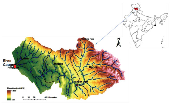
Figure 1.
Map of Beas river basin.

Table 1.
Summary statistics of the P (mm/day), (mm/day), and T C for the Pong sub-catchments.
4. Research Methodology
4.1. The Methodological Framework of the HMM_GP Model
The methodological framework of the HMM_GP model consists of four stages and is illustrated in Figure 2, as adapted from [58]. The colour schematics applied in Figure 2 represent the key four stages of the HMM_GP modelling framework which are briefly described below and can found elsewhere [58] for underlying technical details. Grey colour boxes are used for highlighting data pre-processing and post-processing steps, whereas purple boxes indicate the start and end of the procedure.
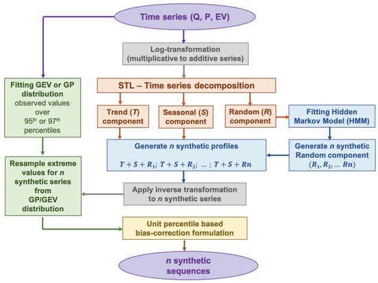
Figure 2.
Work flow diagram of HMM_GP model, adapted from [58].
- Stage 1 (Orange)—Time series decomposition using a robust STL (a seasonal-trend decomposition procedure based on Loess) [59]: the STL procedure facilitates a temporal decomposition of observed time series (O) into three components: (i) long-term trends (); (ii) seasonal movements (S); and (iii) random variations(R).Since the STL procedure is mostly suitable for additive decomposition, input time series are recommended for a log transformation. The data pre-processing is intended to stabilise variance in non-stationary series and to de-emphasise the influence of extreme values (outliers). A detailed literature review covering a detailed overview of the STL method, along with other closely related mathematical techniques for time series decomposition, such as empirical mode decomposition (EDM), can be found elsewhere [58,60,61].
- Stage 2 (Blue)—Fitting of the hidden Markov model (HMM) to the random component: application of the HMM model to the random component facilitates the simulation of uncertainty/randomness associated with the process. The theoretical structure of the HMM model is comprised of five components, as represented in Table 2. Table 2 also details the procedure of fitting the HMM model to the random component used within the HMM_GP framework.
Table 2. Structural composition of HMM.The HMM model fitted to the random component is used to simulate n− user-specified random components. These synthetic random components are then combined with the trend and seasonal components of the observed series to construct n synthetic time series corresponding to the original series.
- Stage 3 (Green)—Fitting GEV or GP distribution: to effectively simulate extreme values, a GEV or GP distribution is fitted to extreme values, specifically in the range of 95th–99.9th percentiles, in the observed series. All synthetically simulated series are then processed to resample extreme values from the fitted distribution. This step ensures that the extreme limits of the synthetic sequences are not constrained by the observed dataset and the fitted continuous distribution allows to incorporate unseen extreme events in the synthetic series. A technical discussion on the appropriateness of selecting a GEV or GP distribution can be found elsewhere [62].
- Stage 4 (Yellow)—Bias Correction: data transformation procedure involving log-transformation and back transformation often produces biased predictions [63]. To minimise the influence of the data transformation procedure, a novel percentile-based bias correction is applied to synthetic series so that synthetic data are not out of synch with actual data.
Following the HMM_GP approach, as detailed above and illustrated in Figure 2, we seek to generate synthetic streamflow sequences for the river inflow data Q, and similarly for the and P time series. We aim to both show that (a) our synthetic stream flows have the same statistical dynamics and characteristics as the actual dataset; and (b) provide future stream flows to investigate the effect of greater disturbance from ENSO events on the agriculture industry in India.
The underpinning methodology for the generation of synthetic time series for Q, and P remain the same, though the procedure needs to be adapted to incorporate slight variations noted in the different dataset due to the difference in the quantitative nature of the data. For example:
- (a)
- Time series of has a considerably small range, , and does not exhibit an overly long-tailed distribution (long-tailed or heavy-tailed distributions are those with extended tails in either the right or left or both directions, due to several values occurring far from the mean or central part of the distribution. Long-tailed distributions are mainly studied within the context of extreme value distribution). However, the time series of the dataset does not exhibit an overly long-tailed distribution. Therefore, to process the dataset requires some adaptation in Stage 3. Specifically, we chose to fit a GEV distribution rather than a GP type distribution in the observed time series of , as detailed in [62].
- (b)
- Time series of P has a wide range of values with many zero values and a long-tailed distribution. For the time series of P, as there can be valid zero elements of the series, we shift the series by a very small translation, 0.001, so that we can take the of the series. As the data are available in two decimal places and range from 0.01 to 136.83, this small value does not represent a significant change to the data and does not excessively stretch (on the negative side) the range of values that the log of the series takes (note this is significant when fitting an HMM to the data). Stages 1 and 2 are applied, and after transforming the synthetics series, we subtract the small shift value, 0.001, from the synthetic series. In contrast to the data, in Stage 3, as the distribution for the P data is very long-tailed, thus, we choose to fit a GP distribution.
- (c)
- The time series of Q has a very wide range, , and a long-tailed distribution. A climatic module is developed to integrate the influence of and P data in simulated Q sequences, detailed in the next subsection.
4.2. Calibrating ‘Climatic Module’ for Simulating Q Sequences
In a novel approach, we seek to link the underlying data trend for Q with underlying climatic conditions, noting that , as measured by the Penman–Monteith method, depends on daily mean T, wind speed, relative humidity and solar radiation [16]. We thus investigated fitting a model for the response of the trend for the Q series to changes in the trend for P and as follows:
- 1
- We take the log of the Q time series to convert a multiplicative time series into an additive series.
- 2
- Using the Loess method of time series decomposition from [59], we decomposed the series into trends, seasonality, and random components.
- 3
- We fit a linear regression model for the response of the decomposed trend of the series to the trends generated by decomposition of and , as described in Section 4.1 above:Accordingly, we complete the generation of n synthetic series for the Q data complementing the synthetic series generated for P and with the following steps:
- 4
- We fit an HMM to the of random component.
- 5
- Using the HMM, we generate the prescribed number of synthetic random series for a pre-determined length of time (less than or equal to that of the P and length).
- 6
- We recombined the decomposed series by adding the seasonality component for the from Step 2 and the trend fitted by the linear regression model to each of the N synthetic random series from Step 5.
- 7
- Take the exponential of each of the N resultant series from Step 6.
- 8
- Re-sample extreme values in the synthetic series from a GP distribution fitted to the extreme values in the actual Q data, as detailed in Stage 3. As the distribution for the Q data is very long-tailed, we choose to fit a GP distribution and apply Stage 4 from Section 4.1.
4.3. Application of ‘Climatic Module’ for Forecasting Q Sequences
Further to generating synthetic Q series for a particular time frame using HMM to ‘learn’ the behaviour of the random component over that time, we also investigated how feasible it would be to use our synthetic series to predict future Q, dependent on climate changes. For this exercise, we proposed using a truncated portion of the Q data to ‘learn’ the behaviour of the Q data to predict the Q for the future. In this way, we can compare our predictions with actual river runoff data. We do this through the following steps:
- 1
- We split the time-frame T for our data into two segments and , such that the start date in the year for both and is the same (to ensure the correct starting probabilities for our fitted HMM). Note we also assume that .
- 2
- For the inflow data in the time-frame, we follow the initial steps for generating synthetic inflow series up to fitting an HMM to the random decomposed series, including generating the linear regression model for the trend on the time period .
- 3
- Using the HMM fitted for the inflow data in the time period generates the prescribed number (N) of synthetic random series for the time period .
- 4
- For the manufacture of the synthetic Q series for time period by adding the predicted random series, the predicted trend for the Q uses the linear model whose parameters are fitted from the data in the time period and generated using the P and trend from time period , and the seasonal inflow component is generated by using the annual seasonal component decomposed in the time period .
- 5
- Take the exponential of each of the N resultant series.
- 6
- Re-sample extreme values in the synthetic series from a GP distribution fitted to the extreme values in the actual Q data, as detailed in Stage 3, and apply a percentile bias, as detailed in Stage 4.
5. Results
This section aims to demonstrate and discuss the key results obtained at various stages of model development (detailed in the above section). Key research findings are organised in four subsections discussed below.
5.1. STL Decomposition of , P and Q
To demonstrate the results obtained at Stage 1 of the HMM_GP framework, Figure 3, Figure 4 and Figure 5 show the STL decomposition for the log of the time series for , P and Q, respectively, during the period from 1998 to 2010. Note that as zero entries may occur in the data for P, before taking logs, we add a very small number () to the P time series. A reverse of this is performed when transforming back from the additive series to the multiplicative series. We set the seasonal decomposition window to a granularity of one year as we wish to investigate the changes on an annual basis. Both and Q show clear annual peaks and troughs, whereas the P, although exhibiting an annual monsoon season, has many days throughout the year when there is either zero or extremely low rainfall. We can see that, in general, the trend for , and exhibit a change in behaviour around the years 2003–2004 where Q shows a change in decreasing trend to increasing trend; P shows levelling off after years of increasing, and starts a downward trend after a few years of a generally unchanging trend. Therefore, we concluded that, in general, as the trend for decreases, we expect an increase in the trend for Q into the reservoir. We also see that as the trend for P increases to its peak in 2006, the trend for Q also rises. Please note that the periods of 2002–2003, 2004–2005, 2006–2007 and 2009–2010 were recorded to observe ENSO events [64].
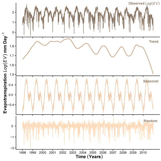
Figure 3.
STL decomposition of .
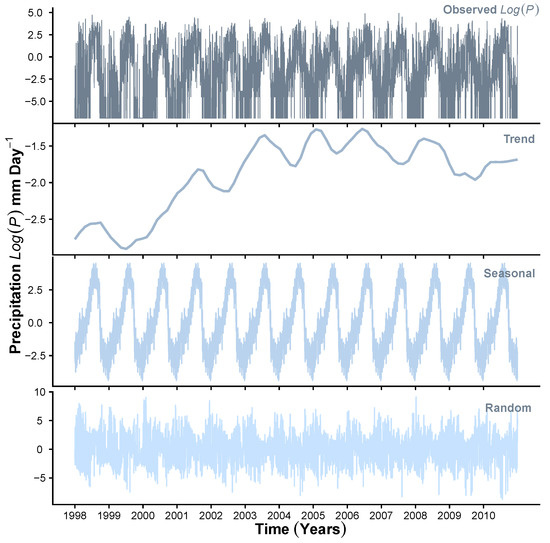
Figure 4.
STL decomposition of .
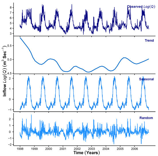
Figure 5.
STL decomposition of .
5.2. Calibration of the HMM_GP Model for Simulating Synthetics Sequences
We applied HMM_GP methodology to simulate synthetic sequences for , P and Q. Figure 6 and Figure 7 show a sample synthetic series generated using the HMM_GP methodology for and P, respectively, during the period from 1998 to 2010, and Figure 8 shows a sample synthetic series for inflow (Q) during the period from 1998 to 2006. The synthetic time series exhibits good agreement with periodic peaks and troughs of the observed data (Figure 6a, Figure 7a and Figure 8a), although since our modelling is based on probabilities, the most extreme values in the synthetic series do not always match the years in the original Q time series when the most extreme events occur. Notably, as and Q both have clear annual peaks and troughs, the modelled synthetic data show better agreement with annual timings of highs and lows than for P. The percentiles and probability density function for the synthetic series follow the observed time series reliably (Figure 6b,c, Figure 7b,c and Figure 8b,c) and the quantile–quantile plot in Figure 6d, Figure 7d and Figure 8d show good agreement, particularly below the 99th percentile. Figure 6e,g, Figure 7e,g and Figure 8e,g show the auto-correlation and partial auto-correlation over a lag time of 1 month for the actual data for , P and Q, respectively, with their counterparts for the synthetic series shown in Figure 6f,h, Figure 7f,h and Figure 8f,h. There is a good agreement for each of the synthetic series with actual data, and we also note that both and Q show a higher level of auto-correlation in general (Figure 6e,f and Figure 8e,f) when compared with P (Figure 7e,f).
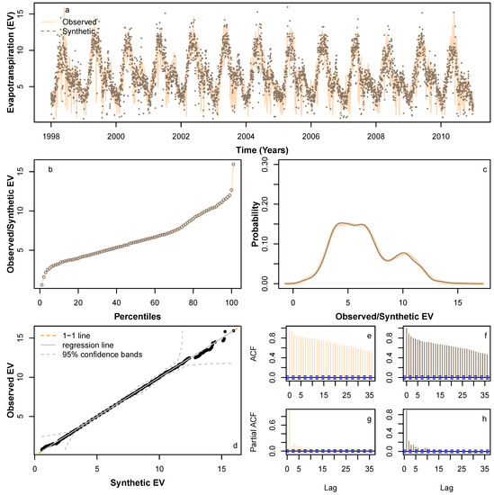
Figure 6.
Comparison of various statistical characteristics of a sample synthetic time series during the period 1998–2010 (dotted brown lines), based on learning pattern from 1998 to 2010, with observed 1998–2010 time series (solid peach lines): Comparing (a) realisation; (b) percentiles; (c) probability density distribution; (d) QQ-plot; (e) ACF for observed; (f) ACF for a sample synthetic series; (g) PACF for observed; and (h) PACF for a sample synthetic series.
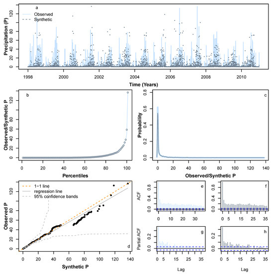
Figure 7.
Comparison of various statistical characteristics of a sample synthetic P time series during the period 1998–2010 (dotted lines in slate grey), based on a learning P pattern from 1998 to 2010, with observed P 1998–2010 time series (solid lines in light slate grey). Comparing (a) realisation; (b) percentiles; (c) probability density distribution; (d) QQ-plot; (e) ACF for observed; (f) ACF for a sample synthetic series; (g) PACF for observed; and (h) PACF for a sample synthetic series.
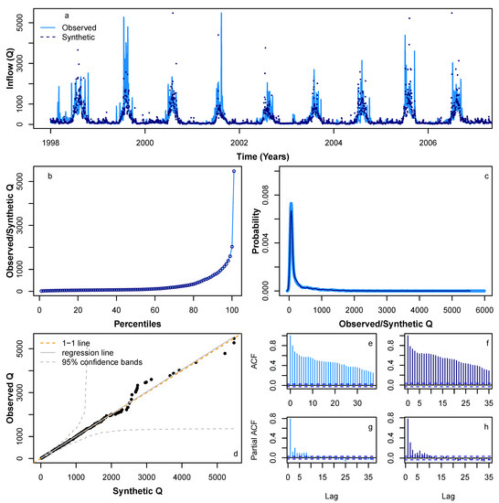
Figure 8.
Comparison of various statistical characteristics of a sample synthetic Q time series during the period 1998–2006 (dotted navy lines), based on learning Q pattern from 1998 to 2006, with observed Q 1998–2006 time series (solid blue lines). Comparing (a) realisation; (b) percentiles; (c) probability density distribution; (d) QQ-plot; (e) ACF for observed; (f) ACF for a sample synthetic series; (g) PACF for observed; and (h) PACF for a sample synthetic series.
To fit extreme values adequately in the synthetic series, we found that fitting the GEV distribution to extreme data values above the 95th percentile provided the best results. For fitting the GP distribution to the precipitation data, we also found that fitting to data above the 95th percentile was optimal, whereas for the Q data, we found that fitting to the 99th percentile was the best option. We suspect that fitting our model to a time series with a lower degree of auto-correlation is more problematic due to the greater likelihood of large differentials between sequential data points. In our case study, this is due to the nature of P data that can change from high to low on a daily basis even during monsoon season. There is ample room for further investigation in this area.
Figure A1, Figure A2 and Figure A3 (provided in Appendix A) show a further four sample synthetic series generated using HMM_GP for , P, and Q, respectively, each exhibiting similar statistical properties to those in Figure 6, Figure 7 and Figure 8. We conclude that the synthetic series we produced for , P, and Q has similar statistical characteristics to their original series. Thus, the HMM_GP framework is shown to effectively simulate the dynamics of the climatic variable along with river runoff. In fact, in earlier work by the authors, the proposed modelling schematic was shown to generate statistical synthetics time series for a range of applications including energy demand series at different resolution in the range of 5–30 min [58] and for Scottish rivers inflow sequences (15 min inflow) [17]. In the present work, the model is first applied to simulate the statistical dynamics of climatic variables, then a novel climate module is developed.
5.3. Calibration of ‘Climatic Module’
The climate module is a novel feature of the HMM_GP model intended to establish a mathematical association between the trend components of climatic variables ( and P) with the trend of (Q) using a simple multiple regression-based models. The key underpinning idea is that such a relationship can be used to project changes in the trend of future Q as a response to change in and P. The seasonal component can be explored with the same conceptual framework, though it is not the focus of the present work. The output from R [65] for the linear model linking the trend of to the trend of and trend of gives the following model summary:
Call:
lm(formula = Trend_TS_Inflow_Log ~
Trend_TS_PrecL_Log + Trend_TS_EvoPL_Log)
Residuals:
Min 1Q Median 3Q Max
−0.22324 −0.06903 −0.00638 0.06717 0.16561
Coefficients:
Estimate Std. Error t value Pr(>|t|)
(Intercept) 12.235107 0.049441 247.5 <2e−16 ***
Trend_TS_PrecL_Log −0.288592 0.002832 −101.9 <2e−16 ***
Trend_TS_EvoPL_Log −4.416697 0.028030 −157.6 <2e−16 ***
---
Signif. codes: 0 ‘***’ 0.001 ‘**’ 0.01 ‘*’ 0.05 ‘.’ 0.1 ‘ ’ 1
Residual standard error: 0.08359 on 3282 degrees of freedom
Multiple R-squared: 0.8992, Adjusted R-squared: 0.8992
F-statistic: 1.465e+04 on 2 and 3282 DF, p-value: < 2.2e−16
where we can see that the linear model we proposed is a reasonable fit as the residual standard error is low and the p-values for both P and are extremely small (less than 0.05) and suggest that both P and in the model are statistically significant and we should retain them. The R-square values is 0.89∼0.9, which is considerably high, suggesting a ’strong’ model fit has been achieved. The overall p-value of the regression model is also small (less than 0.05 as indicated in the last row), suggesting that modelling is statistically significant. To assess the capabilities of the ‘climate module’ in simulating trend components of Q, the upper panel in Figure 9 compares the results for the modelled Q trend (dashed lines in light blue) superimposed on the observed Q trend (solid line in navy), showing a reasonable model fit. We note that the fit is not perfect, in particular, that the peaks and troughs in the trend are not always concurrent. However, the overall general trend is followed with good agreement. To further analyse the discrepancies in the match and the magnitude, in lower panel of Figure 9, we plotted the histogram of residual errors (defined as the difference between the ‘observed’ and ‘predicted’ trend of Q). It is interesting to notice that most of the residual error (approximately ) is distributed within the range of with some extreme values reaching the range . Table 3 provides a detailed percentile distribution of residual error.
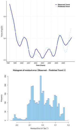
Figure 9.
Upper panel: Compares observed trend component of (solid lines in Navy) with predicted trends of during the period 1998–2006 simulated by ‘climate module’ (dashed lines in light blue) in response to trend of and as independent variables. Lower panel: histogram of residual error distribution.
Table 3.
Percentiles for residual error.
In future versions of our work, we intend to improve this model and consider this further in the final discussion, in particular considering possible lags in the data.
5.4. Model Prediction
Figure 10 shows the predicted Q from 2007 to 2010 based on learning the behaviour of the Q time series during the period 1998–2006 based on the STL seasonal decomposition, using an HMM to learn the random component during the period 1998–2006 and the linear model for the Q trend whose coefficients are found using the P and trend data during the period 1998–2006. The resultant predicted Q for 2007–2010 closely follows the timing of peaks and troughs of the original data (Figure 10a). Due to our modelling being on a probabilistic basis, the most extreme values in the synthetic series do not always match the years in the original Q time series when the most extreme events occur. However, the percentiles (Figure 10b), probability density (Figure 10c), ACF, and PACF profiles (Figure 10e–h) have a similar statistical profile to the original series. Figure 11 shows a further four sample synthetic series for Q, each exhibiting similar statistical properties to those in Figure 10. Therefore, we showed that for several years (less than the initial learning period), we can predict the vast majority of the behaviour exhibited by the original series, bar-identifying the correct years when the most extreme events occur.
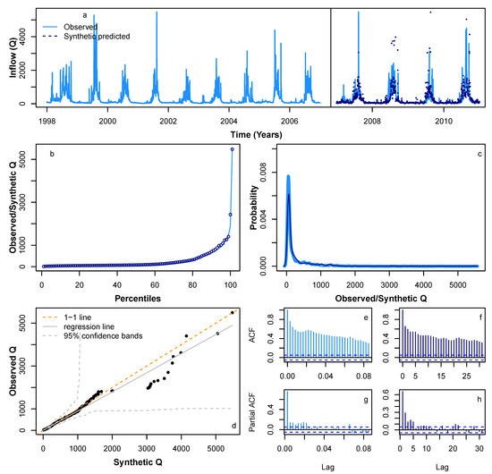
Figure 10.
Comparison of various statistical characteristics of a sample predicted Q during the period 2007–2010 (dotted navy lines), based on learning inflow pattern from 1998 to 2006, with observed Q 2007–2010 time series (solid blue lines). Based on learning Q during the period 1998–2006, comparing (a) realisation of observed Q time series during the period 1998–2010 (solid blue lines) and a sample predicted time series during the period 2007–2010 (dotted navy lines); (b) percentiles for observed Q time series (solid blue lines) and a sample predicted time series during the period 2007–2010 (dotted navy lines); (c) probability density distribution for observed Q time series (solid blue lines) and a sample predicted time series during the period 2007–2010 (dotted navy lines); (d) QQ-plot for observed Q time series (solid blue lines) and a sample predicted time series during the period 2007–2010 (dotted navy lines); (e) ACF for observed Q 2007–2010 time series; (f) ACF for a sample predicted Q 2007–2010 time series; (g) PACF for observed Q 2007–2010 time series; and (h) PACF for a sample predicted Q 2007–2010 time series.
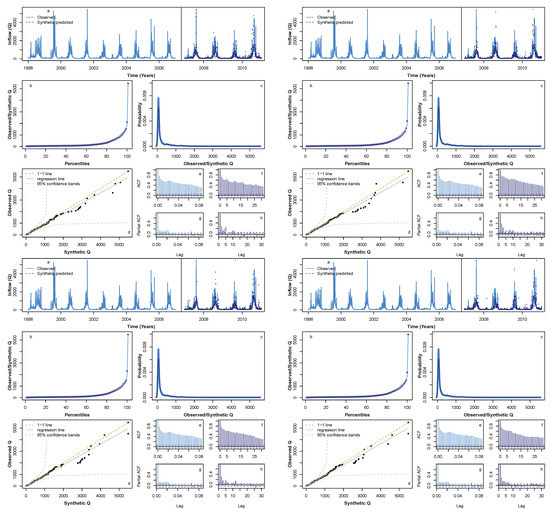
Figure 11.
Comparison of four sample predicted inflow time series during the period 2007–2010. This figure is aimed to illustrate the performance of model for additional four samples and is a cluster of four subfigures that contains 8 subsubfigure each (listed as a–h) for consistency. See Figure 10 for individual subsubfigure details.
5.5. Model Application: Uncertainty in Reservoir Capacity Estimates
The required capacity to meet the existing demands at the Pong without failure is explored using the different Q scenarios. A simple technique for obtaining the failure-free capacity estimate is the sequent peak algorithm (SPA) proposed by [63]
where is reservoir capacity, band are, respectively, the sequential deficits at the end and start of time period t, is the demand during t, is the inflow during t and N is the number of months in the data record. The SPA is a critical period reservoir sizing technique and like all such techniques assumes that the reservoir is full at the start and end of the cycle, i.e., . If, however, this is untrue, i.e., , the SPA cycle is repeated by setting the initial deficit to , i.e., . This second iteration should end with unless the demand is unrealistic, e.g., such as attempting to take a demand higher than the mean annual runoff from the reservoir. In this sense, the assumption of an initially full reservoir is not crucial for the SPA because if this assumption is not valid, it will become evident at the end of the first cycle and corrected for during the second cycle.
To estimate uncertainty in reservoir capacity, the HMM_GP model along with the ‘climate module’ is applied to generate 1000 synthetic Q sequences. The population of reservoir capacity based on existing monthly irrigation releases at the Pong is summarised in Figure 12. The horizontal dashed line represents the existing (or historic) capacity of 7290 Mm. As Figure 12 clearly shows, there is wide variability in the required reservoir capacity for each runoff scenario. Although the existing capacity of the Pong is 7290 Mm, the required capacity estimates based on the simulated current runoff series could be as low as 3545 Mm or as high as 21,452 Mm. These, respectively, represent under-design and over-design situations relative to the existing capacity at the Pong reservoir. The implication of under design is that the reservoir will frequently fail to meet the demand.
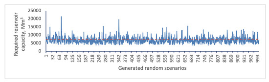
Figure 12.
Reservoir capacity uncertainty using the generated random inflow scenarios.
The effect of ENSO on the capacity estimates broadly follows the effect on runoff. Thus, as the rainfall and hence runoff decreases, the capacity required for meeting the demand increases. The large array of possibilities in the impact of ENSO are bound to complicate decision-making regarding adaptation and mitigation.
6. Discussion
From the initial data that we obtained for the Beas river basin (, P and Q), we demonstrated that we can successfully produce a suite of synthetic time series exhibiting similar statistical characteristics to the original historic data, following seasonal highs and lows well. Moreover, we linked the trend of the Q to the Pong dam to local P and . Using this link to the trend in climatic conditions, we also demonstrated that predictions for inflow based on seasonality and random flow learnt from historical river Q data and climatic trend are statistically accurate. With the ability to adjust the Q trend based on the amount of P and other climatic conditions, we envisage that such synthetic time series can be used as input to crop growth models to help understand the effects of changes in climatic factors on crop selection and output. We based this work on data available for the river Beas in the north of India and this approach can easily be translated to other rivers in India influenced by monsoon conditions and extreme weather events. Of course, this depends on good quality historical data on which accurate machine learning can be built.
The accuracy of our model depends on a suitable length of historical data to train data to capture long-term changes in patterns. In the case study, we predicted 4 years of Q based on 9 years of learning. Given that ENSO type events can occur every 2–7 years and have a variable duration, we would expect more accurate results with historical data that include multiple numbers of ENSO type occurrences. We envisage that if the learning phase of our model has a longer duration, then our model will have a greater likelihood of simulating extreme value occurrences.
As well as the length of data, extending the breadth of data used for historical learning may also improve prediction results. In this study, we limited the linking of the trend of the Q to the and P in the Beas river basin (up to the Pong dam), and it is conceivable that other explanatory variables may improve the linear model for the Q trend (Figure 9). We know that P in the uppermost reaches of the river Beas falls as snow during the winter months, and that snowmelt significantly contributes to Q [66]. If sufficient historical data for and P in the upper reaches of the river Beas are available, further investigation to fitting a multiple linear regression model to and P from a wider catchment could be beneficial. Note that this would also require an understanding of any time lag that occurs between effects of and P in the upper catchment area and the river Q at the Pong dam.
Although the data used for our studies were decomposed using the statistical STL approach, there could perhaps be more deterministic ways of extracting the various components from the data. For instance, if we consider the seasonal patterns in the data that occur over fixed periods, one could use tools such as Fourier and Wavelet transforms for analysis. The data could also be pre-conditioned with such transforms to provide a way to filter noise, or even compress the data. Data decomposed with Fourier/Wavelet transforms could provide a robust method not only to study the present regularities, but also to produce synthetic data that could be used for predictions. The challenge in this aspect of research would be to maintain the statistical properties of the data before and after such a transform. Moreover, Fourier analysis in particular is restricted to finite energy functions, which may interfere with the long-term progression trend of the data. Nonetheless, we could devise techniques to tackle such issues and produce hybrid methodologies to better analyse and model the data [67].
Linked to exploring further avenues for decomposing the data, we note that our modelling approach has been to restrict the STL decomposed seasonal component to be unchanged over each year. It is conceivable that this is too restrictive, and there could be a benefit in allowing the seasonal component to evolve over a period of time. However, such a change would also require changes in the assembling of our inflow predictions. The suggestions we have discussed here provide several future possibilities to extend our statistical modelling approach. As the motivation for modelling runoff is to provide suitable input to ascertain the probabilities of crop success in the face of ENSO type events, the biggest determinant of the most suitable improvements to investigate in the future will be the utility of the synthetic and predicted series in crop development models.
Author Contributions
S.P. contributed in conceptualization, methodology, R coding for HMM model (software), visualization, resources, writing—original, review and editing, supervision, project administration and funding acquisition (Principal Investigator). E.T. contributed in methodology, R coding for climate module (software), investigation, formal analysis, visualization, writing—original draft preparation. B.-S.S. contributed in resources, data curation, writing—lead subject specific sections, supervision, project administration and funding acquisition (Co-Investigator). B.S. contributed in supervision, project administration and funding acquisition (Co-Investigator). All authors have read and agreed to the published version of the manuscript.
Funding
This work is funded by GCRF Scottish Government (Heriot-Watt Internal) funded project "Understanding Impacts of EL Niño events on the Indian Agricultural Productivity (UNITE)", 1 April 2019–September 2019.
Institutional Review Board Statement
The authors confirm that this research does not involve any animal and humans participants.
Informed Consent Statement
The authors confirm that this research does not involve any humans participants.
Data Availability Statement
The authors confirm that the data used in this study are well-referenced within the article and can be accessed to generate the results presented.
Acknowledgments
We would like to thanks Mayank Drolia (TCM Group, Cavendish Laboratory, University of Cambridge, Cambridge, CB3 0HE UK) and Renji Remesan (School of Water Resources, Indian Institute of Technology, Kharagpur, India - 721302) for their contribution in project meeting and discussion.
Conflicts of Interest
The authors declare no conflict of interest. The authors confirm that the work presented in this paper is free from conflict of interest in any form of personal, commercial or financial nature.
Nomenclature
| Evapotranspiration | |
| P | Precipitation |
| T | Temperature |
| ANN | Artificial neural network |
| BBMB | Bhakra Beas Management Board |
| DBN | Deep belief network |
| ENSO | El Niño/Southern Oscillation |
| GEV | Generalised extreme value |
| GP | Generalised Pareto |
| HMM | Hidden Markov model |
| IMD | Indian Meteorological Department |
| Q | Inflow sequences |
| R | Random |
| S | Seasonal |
| SVR | Support vector regression |
| Tr | Trend |
| USGS | U.S. Geological Survey |
| WANN | Wavelet-based Artificial neural network |
Appendix A

Figure A1.
Comparison of four sample synthetic time series during the period 1998–2010. This figure is aimed to illustrate the performance of the model for additional four samples and is a cluster of four subfigures that contains 8 subsubfigure each (listed as a–h) for consistency. See Figure 6 for individual subfigure details.


Figure A2.
Comparison of four sample synthetic P time series during the period 1998–2010. This figure is aimed to illustrate the performance of the model for additional four samples and is a cluster of four subfigures that contains 8 subsubfigure each (listed as a–h) for consistency. See Figure 7 for individual figure details.


Figure A3.
Comparison of four sample synthetic Q time series during the period 1998–2006. This figure is aimed to illustrate the performance of the model for additional four samples and is a cluster of four subfigures that contains 8 subsubfigure each (listed as a–h) for consistency. See Figure 8 for individual figure details.

References
- Gleick, P.H. Streamflow and the Water Cycle. In Encyclopedia of Climate and Weather; Oxford University Press: New York, NY, USA, 1996; pp. 817–823. [Google Scholar]
- Johnson, A.C.; Acreman, M.C.; Dunbar, M.J.; Feist, S.W.; Giacomello, A.M.; Gozlan, R.E.; Hinsley, S.A.; Ibbotson, A.T.; Jarvie, H.P.; Jones, J.I.; et al. The British river of the future: How climate change and human activity might affect two contrasting river ecosystems in England. Sci. Total Environ. 2009, 407, 4787–4798. [Google Scholar] [CrossRef] [PubMed]
- Robins, P.E.; Skov, M.W.; Lewis, M.J.; Giménez, L.; Davies, A.G.; Malham, S.K.; Neill, S.P.; McDonald, J.E.; Whitton, T.A.; Jackson, S.E.; et al. Impact of climate change on UK estuaries: A review of past trends and potential projections. Estuar. Coast. Shelf Sci. 2016, 169, 119–135. [Google Scholar] [CrossRef]
- Visser-Quinn, A.; Beevers, L.; Patidar, S. A coupled modelling framework to assess the hydroecological impact of climate change. Environ. Model. Softw. 2019, 114, 12–28. [Google Scholar] [CrossRef]
- Walther, G.R.; Post, E.; Convey, P.; Menzel, A.; Parmesan, C.; Beebee, T.J.; Fromentin, J.M.; Hoegh-Guldberg, O.; Bairlein, F. Ecological responses to recent climate change. Nature 2002, 416, 386–395. [Google Scholar] [CrossRef]
- Whitehead, P.G.; Wade, A.J.; Butterfield, D. Potential impacts of climate change on water quality and ecology in six UK rivers. Hydrol. Res. 2009, 40, 113–122. [Google Scholar] [CrossRef]
- Visser-Quinn, A.; Beevers, L.; Collet, L.; Formetta, G.; Smith, K.; Wanders, N.; Thober, S.; Pan, M.; Kumar, R. Spatio-temporal analysis of compound hydro-hazard extreme across the UK. Adv. Water Resour. 2019, 130, 77–90. [Google Scholar] [CrossRef]
- Seneviratne, S.; Nicholls, N.; Easterling, D.; Goodess, C.; Kanae, S.; Kossin, J.; Luo, Y.; Marengo, J.; Mc Innes, K.; Rahimi, M.; et al. Changes in climate extremes and their impacts on the natural physical environment. In Managing the Risks of Extreme Events and Disasters to Advance Climate Change Adaptation; A Special Report of Working Groups I and II of the Intergovernmental Panel on ClimateChange (IPCC); Cambridge University Press: Cambridge, UK; New York, NY, USA, 2012; pp. 109–230. [Google Scholar]
- Walker, G.T. Correlation in seasonal variation of weather. Q. J. R. Meteorol. Soc. 1918, 44, 223–224. [Google Scholar]
- Webster, P.J.; Yang, S. Monsoon and ENSO: Selectively interactive systems. Q. J. R. Meteorol. Soc. 1992, 118, 877–926. [Google Scholar] [CrossRef]
- Webster, P.J.; Magaña, V.O.; Palmer, T.N.; Shukla, J.; Tomas, R.A.; Yanai, M.; Yasunari, T. Monsoons: Processes, predictability, and the prospects for prediction. J. Geophys. Res. 1998, 103, 14450–14451. [Google Scholar] [CrossRef]
- McPhaden, M.J.; Zebiak, S.E.; Glantz, M.H. ENSO as an Integrating Concept in Earth Science. Science 2006, 314, 1740–1745. [Google Scholar] [CrossRef]
- Collins, M.; An, S.I.; Cai, W.; Ganachaud, A.; Guilyardi, E.; Jin, F.F.; Jochum, M.; Lengaigne, M.; Power, S.; Timmermann, A.; et al. The impact of global warming on the tropical Pacific Ocean and El Niño. Nat. Geosci. 2010, 3, 391–397. [Google Scholar] [CrossRef]
- Cai, W.; McPhaden, M.J.; Grimm, A.M.; Rodrigues, R.R.; Taschetto, A.S.; Garreaud, R.D.; Dewitte, B.; Poveda, G.; Ham, Y.G.; Santoso, A.; et al. Climate impacts of the El Niño Southern Oscillation on South America. Nat. Rev. Earth Environ. 2020, 1, 215–231. [Google Scholar] [CrossRef]
- Fan, F.; Dong, X.; Fang, X.; Xue, F.; Zheng, F.; Zhu, J. Revisiting the relationship between the South Asian summer monsoon drought and El Niño warming pattern. Atmos. Sci. Lett. 2017, 18, 175–182. [Google Scholar] [CrossRef]
- Early Warning Early Action Report on Food Security and Agriculture (April–June 2019); Licence: CC BY-NC-SA 3.0 IGO; Food and Agriculture Organization of the United Nations (FAO): Rome, Italy, 2019.
- Patidar, S.; Allen, D.; Haynes, R.; Haynes, H. Stochastic modelling of flow sequences for improved prediction of fluvial flood hazards. Geol. Soc. Lond. Spec. Publ. (Geol. Soc. Lond.) 2018, 488, 205–219. [Google Scholar] [CrossRef]
- Gergis, J.L.; Fowler, A.M. A history of ENSO events since A.D. 1525:implications for future climate change. Clim. Chang. 2009, 92, 343–387. [Google Scholar] [CrossRef]
- Tsonis, A.A.; Hunt, A.G.; Elsner, J.B. On the relation between ENSO and global climate change. Meteorol. Atmos. Phys. 2003, 84, 229–242. [Google Scholar] [CrossRef]
- Trenberth, K.E.; Hoar, T.J. E1 Nifio and climate change. Geophhysical Res. Lett. 1997, 24, 3057–3060. [Google Scholar] [CrossRef]
- Wang, B.; Luo, X.; Yang, Y.M.; Sun, W.; Cane, M.A.; Cai, W.; Yeh, S.W.; Liu, J. Historical change of El Niño properties sheds light on future changes of extreme El Niño. Proc. Natl. Acad. Sci. USA 2019, 116, 22512–22517. [Google Scholar] [CrossRef]
- Stevenson, S.L. Significant changes to ENSO strength and impacts in the twenty? First century: Results from CMIP5. Geophys. Res. Lett. 2012, 39, L17703. [Google Scholar] [CrossRef]
- Bhandari, S.; Kalra, A.; Tamaddun, K.; Ahmad, S. Relationship between Ocean-Atmospheric Climate Variables and Regional Streamflow of the Conterminous United States. Hydrology 2018, 5, 30. [Google Scholar] [CrossRef]
- Bradley, R.S.; Diaz, H.F.; Kiladis, G.N.; Eischeid, J.K. ENSO signal in continental temperature and precipitation records. Nature 1987, 327, 497–501. [Google Scholar] [CrossRef]
- Halpert, M.S.; Ropelewski, C.F. Surface temperature patterns associated with the Southern Oscillation. J. Clim. 1992, 5, 577–593. [Google Scholar] [CrossRef]
- Ropelewski, C.F.; Halpert, M.S. Global and regional scale precipitation patterns associated with the El Niño/Southern Oscillation. Mon. Weather. Rev. 1987, 115, 1606–1626. [Google Scholar] [CrossRef]
- Ropelewski, C.F.; Halpert, M.S. Precipitation patterns associated with the high index phase of the Southern Oscillation. J. Clim. 1989, 2, 268–284. [Google Scholar] [CrossRef]
- Ropelewski, C.F.; Halpert, M.S. Quantifying Southern Oscillation? Precipitation relationships. J. Clim. 1989, 9, 1043–1059. [Google Scholar] [CrossRef]
- Chen, D.; Cane, M.A. El Niño prediction and predictability. J. Comput. Phys. 2008, 227, 3625–3640. [Google Scholar] [CrossRef]
- Clarke, A.J. El Niño physics and El Niño predictability. Annu. Rev. Mar. Sci. 2014, 6, 79–99. [Google Scholar] [CrossRef]
- Dijkstra, H.A.; Petersik, P.; Hernández-Garcia, E.; López, C. The application of machine learning techniques to improve El Niño prediction skill. Front. Phys. 2019, 7, 1–13. [Google Scholar] [CrossRef]
- Ham, Y.G.; Kim, J.H.; Luo, J.J. Deep Learning for Multiyear ENSO Forecasts. Nature 2019, 573, 568–572. [Google Scholar] [CrossRef]
- Tamaddun, K.A.; Kalra, A.; Bernardez, M.; Ahmad, S. Effects of ENSO on Temperature, Precipitation, and Potential Evapotranspiration of North India’s Monsoon: An Analysis of Trend and Entropy. Water 2019, 11, 189. [Google Scholar] [CrossRef]
- Islam, M.N.; Sivakumar, B. Characterization and prediction of runoff dynamics: A nonlinear dynamical view. Adv. Water Resour. 2002, 25, 179–190. [Google Scholar] [CrossRef]
- Jayawardena, A.W.; Lai, F. Analysis and prediction of chaos in rainfall and stream flow time series. J. Hydrol. 1994, 153, 23–52. [Google Scholar] [CrossRef]
- Porporato, A.; Ridolfi, L. Nonlinear analysis of river flow time sequences. Water Resour. Res. 1997, 33, 1353–1367. [Google Scholar] [CrossRef]
- Liu, Q.; Islam, S.; Rodriguez-lturbe, I.; Le, Y. Phase-space analysis of daily streamflow: Characterization and prediction. Adv. Water Resour. 1998, 21, 463–475. [Google Scholar] [CrossRef]
- Dhanya, C.T.; Kumar, N.D. Multivariate nonlinear ensemble prediction of daily chaotic rainfall with climate inputs. J. Hydrol. 2010, 403, 292–306. [Google Scholar] [CrossRef]
- Lu, Z.Q.; Berliner, L.M. Markov switching time series models with application to a daily runoff series. Water Resour. Res. 1999, 35, 523–534. [Google Scholar] [CrossRef]
- Lampinen, J.; Vehtari, A. Bayesian approach for neural networks?review and case studies. Neural Netw. 2001, 14, 257–274. [Google Scholar] [CrossRef]
- Shinohara, Y.; Kumagai, T.; Otsuki, K.; Kume, A.; Wada, N. Impact of climate change on runoff from a mid-latitude mountainous catchment in central Japan. Hydrol. Process. 2009, 23, 1418–1429. [Google Scholar] [CrossRef]
- Halff, A.H.; Halff, H.M.; Azmoodeh, M. Predicting runoff from rainfall using neural networks. In Engineering Hydrology; American Society of Civil Engineers: Reston, VA, USA, 1993; Volume 23, pp. 760–765. [Google Scholar]
- Kabir, S.; Patidar, S.; Pender, G. Investigating capabilities of machine learning techniques in forecasting stream flow. Proceed. Institut. Civil Eng. Water Manag. 2020, 173, 69–86. [Google Scholar] [CrossRef]
- Frigessi, A.; Haug, O.; Rue, H. A dynamic mixture model for unsupervised tail estimation without threshold selection. Exremes 2002, 5, 219–235. [Google Scholar] [CrossRef]
- Embrechts, P.; Kluppelberg, C.; Mikosch, T. Modelling Extremal Events; Springer: Berlin/Heidelberg, Germany, 1997. [Google Scholar]
- Carreau, J.; Naveau, P.; Sauquet, E. A statistical rainfall?runoff mixture model with heavy? tailed components. Water Resour. Res. 2009, 45, 10. [Google Scholar] [CrossRef]
- Chavez–Demoulin, V.; Davison, A.C. Generalized additive modelling of sample extremes. J. R. Stat. Soc. Appl. Stat. Ser. C 2005, 54, 207–222. [Google Scholar] [CrossRef]
- Coulibaly, P.; Bobée, B.; Anctil, F. Improving extreme hydrologic events forecasting using a new criterion for artificial neural network selection. Hydrol. Process. 2001, 15, 1533–1536. [Google Scholar] [CrossRef]
- Comte, L.; Buisson, L.; Daufresne, M.; Grenouillet, G. Climate?induced changes in the distribution of freshwater fish: Observed and predicted trends. Freshw. Ecol. 2013, 58, 625–639. [Google Scholar] [CrossRef]
- Hulme, M. Attributing weather extremes to ? Climate change?: A review. Prog. Phys. Geogr. Earth Environ. 2014, 38, 499–511. [Google Scholar] [CrossRef]
- Thompson, R.M.; Beardall, J.; Beringer, J.; Grace, M.; Sardina, P. Means and extremes: Building variability into community level climate change experiments. Ecol. Lett. 2013, 16, 799–806. [Google Scholar] [CrossRef]
- Woodward, G.; Bonada, N.; Brown, L.E.; Death, R.G.; Durance, I.; Gray, C.; Hladyz, S.; Ledger, M.E.; MIlner, A.M.; Ormerod, S.J.; et al. The effects of climatic fluctuations and extreme events on running water ecosystems. Philos. Trans. R. Soc. B (Biol. Sci.) 2016, 371, 20150274. [Google Scholar] [CrossRef]
- Abrahams, C.; Brown, L.; Dale, K.; Edwards, F.; Jeffries, M.J.; Klaar, M.; Ledger, M.E.; May, L.; Milner, A.M.; Murphy, J.A.; et al. The impact of extreme events on freshwater ecosystems. In Ecological Issues Special Publication; British Ecological Society: London, UK, 2013. [Google Scholar]
- Adebayo, A.J.; Soundharajan, B.S.; Ojha, C.S.P.; Remesan, R. Effect of hedging-integrated rule curves on the performance of the Pong reservoir (India) during scenario-neutral climate change perturbations. Water Resour. Manag. 2016, 30, 445–470. [Google Scholar]
- Soundharajan, B.S.; Adeloye, A.J.; Remesan, R.; Ojha, C.S. Simulating the performance of the Pong Reservoir in India under climate change perturbations. In Proceedings of the Dooge-Nash International Symposium, Dublin, Ireland, 24–25 April 2014. [Google Scholar]
- Ncube, S.; Beevers, L.; Adeloye, A.; Visset, A. Assessment of freshwater ecosystem services in the Beas River Basin, Himalayas region, India. In Proceedings of the International Association of Hydrological Sciences—8th International Symposium on Integrated Water Resources Management 2018, Beijing, China, 13–15 June 2018. [Google Scholar]
- Prasad, V.H.; Roy, P.S. Estimation of Snowmelt Runoff in Beas Basin, India. Geocarto Int. 2005, 20, 41–47. [Google Scholar] [CrossRef]
- Patidar, S.; Jenkins, D.P.; Peacock, A.; McCallum, P. A hybrid system of data-driven approaches for simulating residential energy demand profiles. J. Build. Perform. Simul. 2021, 14, 277–302. [Google Scholar] [CrossRef]
- Cleveland, R.B.; Cleveland, W.S.; McRae, J.E.; Terpenning, I. STL: A seasonal-trend decomposition. J. Off. Stat. 1990, 6, 3–73. [Google Scholar]
- Huang, Y.; Schmit, F.G.; Lu, Z.; Liu, Y. Analysis of daily river flow fluctuations using Empirical Mode Decomposition and arbitrary order Hilbert spectral analysis. J. Hydol. 2009, 373, 103–111. [Google Scholar] [CrossRef]
- Agana, N.A.; Homaifar, A. EMD-Based Predictive Deep Belief Network for Time Series Prediction: An Application to Drought Forecasting. J. Hydology 2018, 5, 18. [Google Scholar]
- Pender, D.; Patidar, S.; Pender, G.; Haynes, H. Stochastic simulation of daily streamflow sequences using a hidden Markov model. Hydrol. Res. 2015, 47, 75–88. [Google Scholar] [CrossRef]
- Metcalfe, A.V.; Cowpertwait, P.S. Introductory Time Series with R; Springer: New York, NY, USA, 2009. [Google Scholar]
- United States Climate Prediction Center, Historical El Niño/ La Niña Episodes (1950—Present), Maryland, USA. 2019. Available online: https://origin.cpc.ncep.noaa.gov/products/analysis_monitoring/ensostuff/ONI_v5.php (accessed on 12 May 2021).
- The R Project for Statistical Computing. Available online: https://www.r-project.org/ (accessed on 3 February 2021).
- Jain, S.K.; Ajanta, G.; Saraf, A.K. Assessment of snowmelt runoff using remote sensing and effect of climate change on runoff. Water Resour. Manag. 2010, 24, 1763–1777. [Google Scholar] [CrossRef]
- Krishna, B.; Satyaji Rao, Y.R.; Nayak, P.C. Time Series Modeling of River Flow Using Wavelet Neural Networks. J. Water Resour. Prot. 2011, 3, 3778. [Google Scholar] [CrossRef]


Publisher’s Note: MDPI stays neutral with regard to jurisdictional claims in published maps and institutional affiliations. |
© 2021 by the authors. Licensee MDPI, Basel, Switzerland. This article is an open access article distributed under the terms and conditions of the Creative Commons Attribution (CC BY) license (https://creativecommons.org/licenses/by/4.0/).