Hydrological Analysis of Extreme Rain Events in a Medium-Sized Basin

Abstract

The hydrological response of a medium-sized watershed with both rural and urban characteristics was investigated through event-based modeling. Different meteorological event conditions were examined, such as events of high precipitation intensity, double hydrological peak, and mainly normal to wet antecedent moisture conditions. Analysis of the hydrometric features of the precipitation events was conducted by comparing the different rainfall time intervals, the total volume of water, and the precedent soil moisture. Parameter model calibration and validation were performed for rainfall events under similar conditions, examined in pairs, in order to verify two hydrological models, the lumped HEC-HMS (Hydrologic Engineering Center’s Hydrologic Modeling System model) and the semi-distributed HBV-light (a recent version of Hydrologiska Byråns Vattenbalansavdelning model), at the exit of six individual gauged sub-basins. Model verification was achieved by using the Nash–Sutcliffe efficiency and volume error index. Different time of concentration (T_c) formulas are better applied to the sub-watersheds with respect to the dominant land uses, classifying the T_c among the most sensitive parameters that influence the time of appearance and the magnitude of the peak modeled flow through the HEC-HMS model. The maximum water content of the soil box (FC) affects most the peak flow via the HBV-light model, whereas the MAXBAS parameter has the greatest effect on the displayed time of peak discharge. The modeling results show that the HBV-light performed better in the events that had less precipitation volume compared to their pairs. The event with the higher total precipitated water produced better results with the HEC-HMS model, whereas the rest of the two high precipitation events performed satisfactorily with both models. April to July is a flood hazard period that will be worsened with the effect of climate change. The suggested calibrated parameters for severe precipitation events can be used for the prediction of future events with similar features. The above results can be used in the water resources management of the basin.

1. Introduction

The city of Toronto is exposed to severe weather systems, producing occasional flash floods mainly due to various thunderstorms over a district, or slow-moving storms crossing a domain [1]. In a recent study, the spatial and temporal analysis of long-term daily rain data, examining various climate oscillations, revealed that extreme rain events over Canada have become even harsher during the period 1950–2012 [2]. The daily data of five large-scale patterns during the period 1958–2013 indicated that summer and fall precipitation was remarkably increased in the Eastern parts of Canada on average by 36.3 mm and 73.3 mm, correspondingly [3]. The survey of various climate indices calculated by historical spatiotemporal daily precipitation observations across Southern Ontario during a 64-year period demonstrated that extreme rainfall became more frequent [4]. Researchers in another study, using the data of 133 stations all over Ontario, being recorded on average within 26 years, applying the regional time trend methodology for several durations of yearly peak precipitation intensities, concluded that the extreme rainfall intensity raised from 1.25% per decade for a 30 min storm to 1.82% per decade for a 24 h storm [5]. In addition, throughout Ontario, with the use of fifty or more years of raw precipitation data, it was found that short duration events with sub-hourly or less than an hour rainfall intensity displayed greater fluctuation in yearly and monthly peak precipitation values than those of longer duration [6]. Paixao et al. [7] suggested the simultaneous use of remotely sensed radar observations and tipping bucket rain gauges recording, to better identify areas with homogeneous severe precipitation. The effectiveness of radar quantitative precipitation estimates (QPEs) for the assessment of reliable rainfall intensity to be used to hydrological software was also punctuated by Wijayarathne et al. [8].

Many researchers have investigated the hydrological modeling effects of a changing climate for different watersheds across Canada, based on statistical downscaled methods applied to global climate models (GCMs) daily datasets [9] and various emission scenarios [10], as well as bias-corrected data resulting from pairs of regional climate models (RCMs) and GCMs [11]. Bias-corrected daily precipitation data from the future projections of several GCMs and the worse emissions scenario A2 of AR4 identified that days of heavy and very heavy precipitation, as well as very wet and extremely wet days, will probably raise notably on an annual basis at great areas of Ontario [12].

Some studies have focused on combining various hydrological models with statistical post-processing techniques [13] quantifying uncertainty [14], either with ensemble Kalman filter data assimilation [15] or with operational numerical weather predictions [16], to produce long-term or short-range flood forecasting across Canadian watersheds. Other researchers have already used hydrological modeling and focused on analyzing the changes of the areas which are responsible for eventual fluxes across the studied basins of Ontario temporally [17], and at the same time on a spatial basis [18]. Some other studies have followed empirical methods to determine the event hydrologic discharge. The analysis of 18 rainfall events in a small agricultural basin in southern Ontario displayed that the low primary moisture content of the soil in the summer and fall season contributed to infiltration excess, while the high soil moisture in the spring period generated saturation excess, with additional factors affecting the fluctuation of seasonal runoff; components such as total rain height and rain intensity were critical in summer and fall, whereas, in fall, the determinant factors were the total rain height and the rain duration [19]. Urban lands tend to grow in Southern Ontario, affecting their hydrologic behavior to severe precipitation events. The research applied on the Canadian Great Lakes watershed including eleven rivers, in which the empirical hydrological analysis utilized data for a 42-year period, from late May to mid-November, revealed that the percentage of urbanization interacted with the size of the basin, producing scale effects on the total discharge. In addition, the rise of urban cover produced an increment in the acceleration of the discharge [20]. Another research showed that climate change affects the city of Toronto more than future urban growth [21]. Many researchers have used and compared various fully distributed, semi-distributed, or lumped hydrological models to assess their performance or for operational forecasting [22,23,24,25], while others have used several discretization patterns concerning the uncertainty of land classes’ sub-divisions, either different land uses’ and soil classes’ resolutions in hydrological simulations [26,27], for continuous modeling, in different watersheds of Ontario and of wider Canada. In recent years, most of the research community has focused on studies in the Canadian region regarding continuous hydrological simulations rather than single flood event modeling.

In this study, we had two objectives; the first was to collect and group in pairs six different precipitation events with similar characteristics (high rainfall intensity, two noted hydrological peaks, various antecedent moisture conditions) to be hydrologically calibrated and verified by the observed hydrographs at the exit of the sub-basins included to a medium-sized watershed in Canada. The second was to propose a final set of parameters of the most appropriate of two applied hydrological models for each pair of events concerning all the gauged sub-basins, to be representative for future event-based modeling regarding storm events with corresponding hydrometric features. For these purposes, 1 h interval data of precipitation, flow, temperature and evaporation were used, along with the topography extracted by a digital elevation model (DEM) at 30 m regional resolution. The analysis of the hydrometric data was performed to recognize the contribution of peak rainfall intensity, rain duration, precedent moisture, soil saturation, ground imperviousness, as well as the average velocity of peak rainfall to the outcoming time of appearance of observed peak discharges with the recorded time of maximum precipitation intensities. To this aim, detailed land use data of 2010 and soil group features of 2015 were used as well. These attributes are critical to carefully identify soil properties such as percolation and perviousness, which are particularly important for the proper design of the models used. Sensitivity analysis, by changing one parameter at a time, was also conducted to identify the variables that influence the time of occurrence and the magnitude of the simulated peak runoffs. The criteria of model verification were the best performance of the Nash–Sutcliffe efficiency coefficient to obtain valid accordance of the hydrograph’s shaping, and the minimization of the rain volume error (%) index, to achieve a fair water balance. Another comparison concerned the results produced by two calibrated hydrological models, the HEC-HMS (Hydrologic Engineering Center’s Hydrologic Modeling System software), an empirical lumped model, and the HBV-light (a recent version of Hydrologiska Byråns Vattenbalansavdelning software), a conceptual semi-distributed model, which have considerable differences. The effect of further increased intensity and the magnitude of the precipitation on the simulated outflow at the basin’s exit, by using a hypothetical factor of 1.5, was also examined, on the probable account of the awaited raise of intense rainfall events in eastern Canada.

2. Materials and Methods

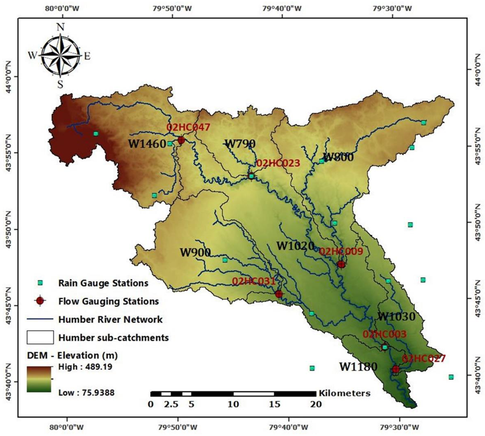
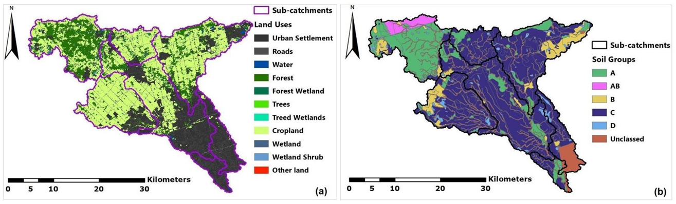
2.1. Study Area: Humber River Basin

The hydrological basin of Humber River is located in the Greater Toronto Area, in Southern Ontario, Canada. The hydrological catchment has an area of 889 km², consisting of seven sub-basins. The area of each sub-basin, along with the length of the longest flow path and its slope, are shown in

Table 1. Characteristics of the Humber sub-watersheds.

Sub-Basin	A (km2)	Longest Flow Path (km)	Slope of Longest Flow Path (m/m)	Flow Gauging Station at Exit
W1460	161.6319	30.490527	0.007277	02HC047
W790	63.2952	15.446972	0.007888	02HC023
W800	192.4848	53.400175	0.003251	02HC009
W900	140.3595	27.587806	0.004841	02HC031
W1030	60.246	31.909755	0.004202	02HC027
W1020	241.1919	76.009458	0.002489	02HC003
W1180	29.8854	19.110794	0.004919	-

.

Figure 1 points out the extent of the Humber River Basin and the existing river network, as resulted through the watershed delineation from the digital elevation model (DEM) at a spatial resolution of 30 m × 30 m, provided by the Ontario Ministry of Natural Resources [28], with the use of the HEC-Geo-HMS extension of ArcGIS. The elevation ranges between 75 m and 489 m above sea level, with the northwest part being characterized as hummocky topography with steep gradients [29], whereas the central part is comparatively flat. For the present study, the Thiessen polygons methodology was used to estimate the mean areal precipitation for each one of the seven sub-watersheds through the weighting of sixteen rain gauges across the total hydrological catchment. Data for the observed flow were used from six flow gauging stations located at the exit of six sub-basins. The observed gauges’ data at 1 h time-step were gathered from the Toronto and Region Conservation Authority [30] and Environment and Climate Change Canada [31]. Based on a 30-year observation period (1971–2000) the average annual precipitation in the basin was found to be equal to 834 mm, according to the records of a station in the City of Toronto, in the shore zone of Lake Ontario [29].

According to the General Land Uses maps of 2010, the watershed studied consists of rural and agricultural uses, urban uses, natural vegetation, and waterbodies. Specifically, the Humber River Basin is covered by urban settlement (28.1%), roads (8.8%), water (0.9%), forest (15.9%), forest wetland (0.4%), trees (0.4%), treed wetlands (0.2%), cropland (44.2%), wetlands (1.0%), wetland shrub (0.1%) and other land (0.01%), as indicated in Figure 2a, afforded by Agriculture and Agri-food Canada, Land Use [32]. Thus, the study watershed is characterized as partly rural and partly urban. In terms of urban settlement, W1460 is 35% high residential, 60% estate residential, and 5% consists of golf course; W790 is 50% high residential and 50% estate residential; W800 consists of 70% high residencies and 30% estate residencies; W900 is 50% high residential, 45% estate residential, and 5% consists of golf course; W1030 is 70% high residential and 30% industrial; W1020 consists of 60% high residencies and 40% industries; W1180 is 100% high residential, based on the interpretation of the joint effort of Civica Infrastructure Inc. (CIVICA) and Toronto and Region Conservation Authority (TRCA) [33] as well as TRCA [34]. As far as roads are concerned, W1460, W790, W800, and W900 consist of gravel roads, paved roads that pass from W1030 and W1180, whereas gravel roads and paved roads exist in W1020 at equal rates, based on the interpretation of [33].

The soil type of the area varies spatially. The soil groups’ map shown in Figure 2b was designed in ArcGIS according to hydrogeological and soil classes’ data, provided by Canadian Soil Information Service, Detailed Soil Survey Compilations [35] and Agriculture and Agri-food Canada, Ontario Detailed Soil Survey [36]. The hydrological soil types met are A, AB, B, C, D, and unclassed, the latter considered to be a mixture of the four soil types (A, B, C, and D) in equal proportions. Soils at Group A have low discharge capacity, accompanied by high percolation rates, whereas soils classified at Group D present high runoff potentiality with low infiltration proportions [37]. The different hydrological soil types found, along with the differentiation of land uses, have an effect on the drainage of each sub-watershed.

2.2. Precipitation Data

Hydrological modeling performance was conducted through the study of six single precipitation events, examined in pairs with similar characteristics. The selected events occurred from 2010 to 2017, mostly during the growing season (spring and summertime). The precipitation was spatially and temporally varying, thus hourly data were collected by sixteen rain gauges across the Humber River Watershed, which thereafter were used to calculate—via gauge weighting—the mean areal precipitation in each of the sub-basins, through the Thiessen polygons methodology. The characteristics that made the examined events significant, studying them in pairs, were: (a) high precipitation intensity in all the sub-basins, higher than 10 mm/h, with values even equal to 25 mm/h, under dry antecedent moisture conditions (AMC Type I); (b) double hydrological peak in a short period, also under dry AMC; and (c) various antecedent moisture conditions, specifically normal (Type II) to wet (Type III) AMC in the predominantly rural sub-basins, whereas dry AMC (Type I) in the urban—for the most part—sub-basins. In all the aforementioned categories, the total amount of precipitated water was greater in the second studied event of each pair. The hydrometric features of the six studied rainfall events examined in pairs, along with the observed peak discharges, are indicated in

Table 2. Characteristics of the studied precipitation events.

No	Event Start	Event End	Modeled Period (h)	Season	Sub-Basins	5-Day Antecedent Moisture Conditions (AMC) (mm)	AMC Type	Total Precipitation (mm)	Max Precipitation Intensity (mm/h)		Observed Peak Discharge (m3/s)		Comments
1	28 May 2013 at 4:00	30 May 2013 at 20:00	64	Growing	W1460	4.6	I	36.6	15.1		6.5		High- intensity event
					W790	3.7	I	36.4	19.0		3.2
					W800	3.5	I	31.9	10.7		15.7
					W900	2.9	I	55.8	25.2		62.1
					W1030	2.1	I	47.8	24.0		122.4
					W1020	3.0	I	48.3	26.0		107.8
2	3 July 2013 at 23:00	10 July 2013 at 23:00	168	Growing	W1460	0.8	I	63.4	10.0		6.5		High- intensity event
					W790	0	I	82.0	25.2		19.3
					W800	0.2	I	81.6	17.9		69.9
					W900	0.1	I	77.2	25.2		81.6
					W1030	0	I	107.3	30.3		201.7
					W1020	0	I	106.7	26.0		268.2
3	7 April 2013 at 5:00	15 April 2013 at 23:00	210	Dormant	W1460	0.9	I	74.2	4.2	9.0	11.0	10.5	2 peaks
					W790	0.5	I	73.6	3.2	5.4	6.1	8.2
					W800	0.2	I	67.1	3.7	8.1	17.1	21.6
					W900	0.5	I	66.9	3.9	8.8	27.8	41.6
					W1030	0.2	I	44.7	2.4	3.5	17.8	14.2
					W1020	0.2	I	60.6	3.3	4.7	84.2	121.3
4	30 April 2017 at 5:00	7 May 2017 at 22:00	185	Growing	W1460	10.3	I	84.1	3.9	3.2	6.1	11.8	2 peaks
					W790	10.1	I	82.0	4.7	2.6	5.4	8.2
					W800	5.5	I	91.4	7.7	2.6	22.6	28.4
					W900	11.3	I	91.2	5.5	3.0	39.6	39.4
					W1030	11.2	I	89.9	4.1	4.8	24.8	15.0
					W1020	8.2	I	86.9	4.6	2.6	90.2	101.5
5	26 June 2010 at 7:00	30 June 2010 at 12:00	101	Growing	W1460	56.7	III	35.3	7.8		6.6		Normal to wet AMC at agricultural lands
					W790	46.5	II	38.3	7.0		4.0
					W800	46.0	II	30.9	4.9		7.6
					W900	38.2	II	35.3	7.9		22.5
					W1030	27.0	I	43.8	24.1		88.4
					W1020	37.8	II → I	41.7	12.2		92.7
6	22 June 2017 at 15:00	25 June 2017 at 17:00	74	Growing	W1460	57.9	III	65.2	16.6		25.5		Normal to wet AMC at agricultural lands
					W790	56.3	III → II	54.5	16.6		13.3
					W800	45.5	II	54.8	13.2		22.4
					W900	35.2	I → II	42.6	11.2		20.7
					W1030	33.8	I	44.9	8.4		61.0
					W1020	38.9	II → I	48.4	10.7		89.4

. Especially for the events of normal to wet AMC at agricultural lands, an adjustment to some of the considered AMC types was assumed, which is one of the factors that determine the curve number (CN), so that there is uniformity in the respective sub-basins of the particular rain events. The limits of rainfall values of the previous five days that specify the type of AMC per season are defined in Section 2.3.

Another important factor for the hydrometric analysis of the examined events is the time difference Δt (h) between the time of the observed peak discharge and the time of the peak precipitation intensity for every monitored sub-basin, which is shown in

Table 3. Time difference between the time of the observed peak discharge and the time of the peak precipitation intensity for the six studied precipitation events.

Event	Δt (h) = Time of Observed Peak Q − Time of Max P
	W1460	W790	W800	W900	W1030	W1020
28–30 May 2013	18	10	6	10	2	14
3–10 July 2013	14	11	13	11	3	15
7–15 April 2013 (1st and 2nd peak)	31	29	34	32	23	29
	13	10	13	10	2	12
30 April–7 May 2017 (1st and 2nd peak)	13	14	18	28	1	13
	27	28	29	13	15	25
26–30 June 2010	17	11	5	13	1	2
22–25 June 2017	7	2	6	9	−4	16

. Considering that Δt is equal to the travel time of the peak rainfall from the basin’s inlet to reach the outlet, expressed by the corresponding flow hydrograph, then Δt (h) is given by the equation:

$$\Delta t=\frac{L\times 1000}{V\times 3600}$$

(1)

where L (km) is the length of the longest flow path of the sub-basin and V (m/s) is the average velocity.

Examining the sub-basin W800 of the first pair of events having high precipitation intensity, regarding the 28–30 May 2013 event, during five days before the storm, the AMC were equal to 3.5 mm, followed by 11.8 mm of rainwater during only 19 h of the precipitation event, which implied that the ground was already saturated before the peak rain intensity. Then, in 1 h, 10.7 mm of rain fell, which was the peak precipitation, and the peak discharge came after 6 h, which is quite reasonable. The resulting average velocity of the peak rain should have been equal to 2.5 m/s, very realistic due to the saturated terrain. On the other hand, concerning the same sub-basin of the 3–10 July 2013 severe rain event, during five days before the storm, the AMC was equal to 0.2 mm. Afterward, during 111 h of the rain event, only 18.8 mm of precipitated water occurred, which signified that there were very dry conditions before the peak rain intensity. Since then, in 4 h fell 58.1 mm of rain, while the 17.9 mm fell only in 1 h, which in total explained the observed peak discharge occurring 13 h after the peak rain intensity. Under these circumstances, the average velocity of the precipitated water should have been equal to 1.1 m/s.

Noticing the second pair of events with the two hydrological peaks, during the 7–15 April 2013 rain event, the interest was focused on the second peak of precipitation intensity which was higher than the first one in all the sub-basins by a factor of 0.42 to 1.26. The raise was not proportional to the peak runoff; specifically, the sub-basins W1460 and W1030 showed a decrease in the peak discharge at the second peak compared to the first one. Moreover, the second peak discharge was higher than the first one in the rest four sub-basins by a factor of 0.26 to 0.50. Generally, in all the watersheds, the time of the first peak discharge was quite delayed in relation to the time of the first peak precipitation height because the precipitated water between the two mentioned times was significant. Indicatively, regarding the sub-basin W1460, the time of the first peak discharge occurred 31 h after the time of first peak precipitation, while in the meantime 21 mm of rain fell. In this case, the resulting average velocity of the peak rain should have been very low and equal to 0.28 m/s. Concerning the 30 April–7 May 2017 rain event, although the first peak precipitation was higher than the second one in nearly all the sub-basins except for W1030, nevertheless, the second peak discharge was higher than the first one in most of the sub-basins, in addition to W1030 and W900. However, in the latter one, the differences were very small, almost indistinguishable. The above observation in most of the sub-basins was because lots of millimeters of rain fell between the second peak precipitation and the second peak discharge. In particular, regarding the sub-basins W1460, W790, and W800, the second peak precipitation intensity was equal to 3.2 mm, 2.6 mm, and 2.6 mm correspondingly, whereas the second peak discharge came after 27 h, 28 h, and 29 h, respectively, after quite enough additional precipitated water to the corresponding sub-basins equal to 35.3 mm, 35 mm, and 32.9 mm. The developed average velocities were particularly low.

Regarding the third pair of events, having normal to wet AMC at the agricultural lands, first of all, the AMC of the sub-basin W1020 of the 26–30 June 2010 event were very close to the upper limit of the dry conditions—and thus were considered as Type I. The same was supposed for the 22–25 June 2017 event. For the latter event, the AMC of the sub-basin W790 were very close to the upper limit of normal conditions, and hence were assumed to be Type II. Moreover, the AMC of the sub-basin W900 were very close to the lower limit of normal conditions, and therefore were regarded as Type II. The above considerations were applied for the uniformity of the initial conditions. Within a more thorough observation of the third pair of events with the 5 days’ AMC classified as normal (Type II), in regard to the sub-basin W790 of the 26–30 June 2010 event, the 5 days’ AMC were recorded as equal to 46.5 mm. After that, at a period of 35 h of the rain event, 18.2 mm of water fell, which did not classify the event as a sudden one, but mostly as one of longer duration. Thereafter, the peak precipitation equal to 7.0 mm that fell afterwards in 1 h justified the reason why the peak discharge occurred 11 h later, which was feasible with an average velocity of the peak rain intensity equal to 0.4 m/s. About the aforementioned sub-basin of the 22–25 June 2017 flash flood event, the AMC—5 days before the event—were recorded as equal to 56.3 mm, followed by 26.3 mm of rain during 15 h of the sudden precipitation event, meaning that the soil became quickly saturated prior to the peak rain intensity. Straight away, 23.3 mm of rainwater fell in 2 h, of which the 16.6 mm precipitated in just 1 h, which in combination interprets the observed peak discharge to be noted just 2 h after the peak rain intensity. That travel time resulted in an average velocity of the peak precipitation equal to 2 m/s. For the sub-basin W1030, a fully urban area, at the 26–30 June 2010 rain event, the 5 days’ AMC equal to 27.0 mm were followed by 9.6 mm of precipitated water during 35 h of the studied event, so the ground was fully saturated thus far due to the high imperviousness. As a result, it is very comprehensible why the time of peak runoff occurred 1 h after the time of peak precipitation of very high intensity, equal to 24.1 mm/h. The resulting travel time of the peak precipitation until the exit of the sub-basin took place with an average velocity equal to 9 m/s. Regarding the event of 22–25 June 2017 and the same sub-basin, there were two peaks of precipitation, one of 7.4 mm and one other—which happened 4 h later—equal to 8.4 mm, that with their turn resulted in two peaks of peak discharge that happened immediately. The first peak discharge was higher and occurred 4 h earlier than the second one. The direct flow was also justified because of the high imperviousness of the urban area, as well as of the high 5 days’ AMC equal to 33.8 mm. The wave’s average velocity was very high as well.

2.3. Hydrological Model HEC-HMS, Setup, and Methods

The Hydrologic Modeling System (HEC-HMS), developed by the U.S. Army Corps of Engineers’ Hydrologic Engineering Center, formed to simulate the precipitation–discharge processes in dendritic catchments such as the Humber River basin, was one of the two models applied to calibrate the six studied single flood events. For the present study, the produced hydrographs resulted from the rain gauge data, with the subtraction of infiltration losses, the transformation of the excess precipitation into surface discharge, and the addition of the baseflow. Open channel flow simulation is also included in the basins required (W1020, W1180) to calculate the output hydrograph [38]. The selected modeling methods for the hydrological response of each sub-basin were: (a) the SCS curve number loss model for counting the cumulative losses; (b) the Clark Unit Hydrograph model for the representation of the basin’s direct runoff via the transformation of excess rainfall; (c) the exponential recession model for counting the basin’s baseflow; and (d) where needed, the Muskingum routing model for the computation of the open channel’s flow [39].

The parameters regarding the SCS Curve Number loss method are the curve number (CN) and impervious (%). The CN is a sensitive parameter used at single flood event modeling, which incorporates the effect of soil type and land use of a watershed, together with the antecedent soil moisture conditions [37]. High residencies are considered as those residential districts by mean lot size equal to 1/8 acre or less, referring to townhouses. Estate residencies are assumed as residential districts by an average lot size of 1/2 acre. Regarding golf courses, these are considered to be in fair hydrologic condition, with grass cover between 50% and 75%. Gravel roads are counted as those that also include right-of-way. Paved roads, together with curbs and storm sewers exclude right-of-way [37]. Water bodies, forest wetland, treed wetlands, wetland, and wetland shrub have a CN equal to 100 at any soil type [40]. Concerning forest, woods are considered to be in fair hydrologic condition, being grazed but not burned, with some forest litter covering the soil. On the other hand, trees are counted as woods and grass (pasture) combination in fair hydrologic conditions and at equal rates. Finally, cropland is considered as row crops planted in straight rows, contoured and terraced, also in fair hydrologic conditions [37]. The hydrologic conditions specify the influence of covering the category on percolation and discharge through components such as canopy, the density of cultivations, quantity of grass, and ground surface coarseness. Poor hydrologic conditions suggest decreased percolation and are prone to raise discharge, whereas good hydrologic conditions point out raised infiltration with a reduced trend of runoff [39]. Curve numbers (CN) per every found land use in the studied sub-basins of the Humber River basin, are given for every met soil group, fair hydrological conditions, and average moisture conditions in [37].

Maps of land use (LU) and soil hydrologic groups (SG) were intersected in ArcGIS, producing a new map that displayed the combination of the above properties. An attribute table that gathered all the data per each unique land use–soil group polygon was constructed, along with every polygon’s area and resulting curve number [37] from the aforementioned joining of land use and soil group, referring to normal (average) runoff conditions (Type II). The final CN of each one of the sub-basins was determined by summing up each resultant CN multiplied with the area-weighted land use-soil group plane element, given as:

$$CN=\frac{{{\displaystyle \sum }}_{i=1}^n\left(A_{i, LU-SG}\times C{N}_i\right)}{A_{total}}$$

(2)

Antecedent moisture conditions (AMC) are defined as the previous 5 days’ rainfall and are important for the computation of the final CN. As with precipitation, so with AMC, the total millimeters of precipitated water in the precedent 5 days in each sub-basin are calculated via the Thiessen polygons methodology. Below are the equations for the CN related to dry conditions (AMC Type I) and wet conditions (AMC Type III), respectively [41]:

$$C{N}_I=\frac{4.2\times C{N}_{II}}{10-\left(0.058\times C{N}_{II}\right)}$$

(3)

$$C{N}_{III}=\frac{23\times C{N}_{II}}{10+\left(0.13\times C{N}_{II}\right)}$$

(4)

For the dormant season, determined from mid-October to mid-April in Canada, AMC are characterized as Type I (dry) for the 5 previous days’ precipitation less than 12.7 mm, Type II (normal) for prior precipitation ranging between 12.7 mm and 27.94 mm, whereas Type III (wet) for precedent precipitated water over 27.94 mm. On the other hand, for the growing season which extends to Canada for about five months, from late April to early October, AMC are referred to as dry for the former 5 days’ rainfall under 35.56 mm, normal for a range between 35.56 mm and 53.34 mm, and wet for more than 53.34 mm [41]. Hence, the AMC ranges affecting the CN are remarkably different among dormant and growing seasons.

The % imperviousness is another important parameter for hydrological modeling. High residencies are considered to have 65% impervious cover. Estate residencies have on average 25% imperviousness [37]. Golf courses are considered pervious. Roads, either gravel or paved, are assumed to be 100% impervious [42]. Industrial districts are 72% impervious [37]. Water bodies, forest wetland, treed wetlands, wetland, and wetland shrub have 0% imperviousness [43]. Both forests and trees are assumed to have 1% impervious cover [44]. Cropland is considered to be 3% impervious [43]. The total % imperviousness of each sub-basin was estimated by the sum of each % imperviousness of one land use multiplied by the area-weighted land use, as given below:

$$\%Total Impervious=\frac{{{\displaystyle \sum }}_{i=1}^n\left(A_{i, LU}\times \%Imperviou{s}_i\right)}{A_{total}}$$

(5)

The final estimated CN as well as the % total imperviousness of every sub-basin are shown in

Table 4. Summary of the Humber sub-basins’ important variables.

Sub-Basin	Curve Number (CN)		% Total Imperviousness	% (Urban Settlement and Roads)	$\frac{\mathit{R}}{{\mathit{T}}_{\mathit{C}}+\mathit{R}}$
	Weighted CNII (Normal Conditions)	CNI (Dry Conditions)
W1460	59	38	8	10.5	0.637
W790	80	63	10	13.1	0.6214
W800	79	61	19	25.8	0.5452
W900	81	64	16	23.1	0.5614
W1030	91	81	73	97.7	0.1138
W1020	85	70	42	54.9	0.3706
W1180	89	77	73	99.5	0.103

.

The parameters that concern the Clark Unit Hydrograph transform method [38] are the time of concentration (T_c) expressing the demanded time so that the precipitated water from the most remote place arrives at the basin’s exit [45], and the storage coefficient (R) indicating the short-lived storage of excess rainfall in the hydrological catchment until it discharges to the exit [39]. Various studies have concluded that the ratio R/(T_c + R) of a watershed is steady, having a value range from 0.1 in the case of an urban catchment runoff to 0.7 in the case of a marshy and flat basin [46]. Thus, supposing that when the ratio is equal to 0.7 it corresponds to 0% urban territory, as well as when the ratio is equal to 0.1 it corresponds to 100% urban area, then the resulting ratios for each sub-basin are displayed in Table 4.

Various empirical equations estimate T_c, taking into account the watershed’s geomorphological characteristics. The empirical formulas which were applied in this study are listed in

Table 5. List of formulas used for the estimation of the time of concentration (h).

Author	Formula	Notes	References
Simas–Hawkins	$T_C=0.0085\frac{A^{0.594}\times {\left(\frac{1000}{CN}-10\right)}^{0.313}}{L^{0.594}\times S^{0.15}}$	Data of 168 basins in USA (0.001–14 km2)	[47,48]
Johnstone–Cross	$T_C=0.4623\frac{L^{0.5}}{S^{0.25}}$	Data of 19 rural basins in USA (A = 64.8–4206.1 km2)	[49]
Williams	$T_C=\frac{0.605\times L}{{\left(100S\right)}^{0.2}\times A^{0.1}}$	Specially recommended to rural basins (A < 137 km2)	[50]
Carter	$T_C=0.0977\frac{L^{0.6}}{S^{0.3}}$	Data of an urban basin in USA (A < 20.72 km2, S < 0.005)	[51]

Notes: Simas–Hawkins is in English units, where A (ft²) is the watershed area, L (ft) is the longest flowpath, and S (ft/ft) is the slope of the longest flowpath. Johnstone–Cross, Williams and Carter formulas are in S.I. units, where L (km) is the longest flowpath, S (m/m) is the slope of the longest flowpath, and A (km²) is the watershed area.

, each one fitting better in sub-basins with specific characteristics.

The parameters regarding the exponential recession baseflow method are the initial discharge per area, the recession constant, and the ratio-to-peak. The recession constant expresses the decay of the baseflow rate among two rain events, determined as the proportion of baseflow at the time being to the specific baseflow which occurred the previous day [38]. The recession constant may take values among 0.3, relating to small basins, and 0.8, regarding large basins [52]. The ratio-to-peak was the preferred process of resetting the baseflow to its initial value throughout a rain event, which will occur at the time that the present baseflow was divided by the highest baseflow decreases at the determined value [38].

The parameters that concern the Muskingum routing method are the Muskingum K (h) expressing the time that the flood wave travels along the channel [38], and the Muskingum X, a dimensionless weighting factor among influx and outflux, ranging from 0 in the case of maximum attenuation in which the flood wave’s shape is flattening to 0.5 in case that there is no attenuation of the rainwater proceeding through the channel [39]. The number of sub-reaches of the channel should also be introduced [38], a parameter that does not cause considerable differences on the flow hydrograph at the exit of the sub-basin, whether the routing system of the channel consists of one reach, or either two or three sub-reaches [53].

The channels from the outlets of the sub-basins W1460, W790, W800, and W900 were routed to the exit of the sub-basin W1020. The corresponding routing channels were named R1580, R1590, R1600, and R1610. In addition, the water channels from the exits of the sub-basins W1030 and W1020 were directed to the outlet of the sub-basin W1180, named R1620 and R590, respectively, while there is no gauging station at this sub-basin’s exit. We assumed that the movement of rainwater through totally agricultural lands with high levels of infiltration may lead to maximum attenuation, corresponding to a Muskingum X equal to 0, whereas in totally urban areas it was considered that there was equal weight among influx and outflux, and the flood wave propagated into the reach uniformly, without attenuation, therefore the Muskingum X was equal to 0.5. The length of the channels, their slopes, as well as the resulting Muskingum X parameter per each channel, are displayed in

Table 6. Characteristics of the channels routed at the exit of the sub-basins W1020 and W1180.

Channel	Length (km)	Slope (m/m)	Muskingum X	Routed to Exit of Sub-Basin
R1580	75.522179	0.001905	0.3	W1020
R1590	51.146611	0.00185	0.3	W1020
R1600	19.12083	0.001358	0.425	W1020
R1610	24.819795	0.00226	0.25	W1020
R1620	7.358818	0.002319	0.45	W1180
R590	12.12955	0.003117	0.45	W1180

.

The output hydrograph at the exit of the sub-basin W1020 results from the water precipitated at the particular sub-basin, as well as the rainwater routed through the channels R1580, R1590, R1600 and R1610. In addition, the flow hydrograph at the outlet of the ungauged sub-basin W1180 was derived from the rain fallen to the specific sub-basin added to the rain directed via the reaches’ channels R1620 and R590.

2.4. Hydrological Model HBV-Light, Setup and Methods

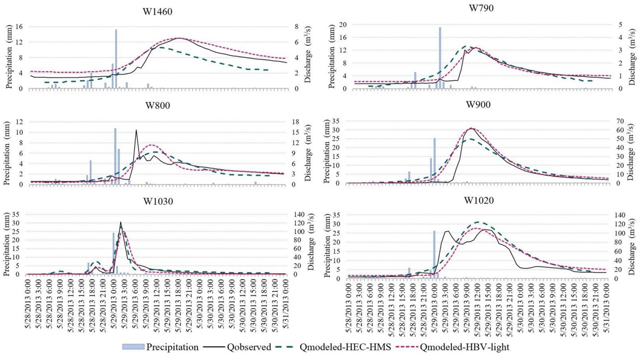
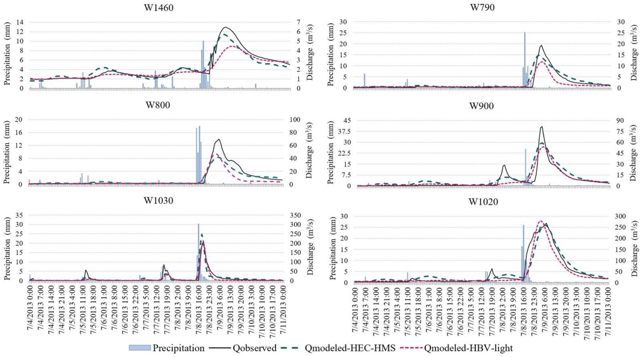
The HBV-light model developed by the University of Zurich, a conceptual semi-distributed model capable of simulating the runoff of a basin comprised of several sub-watersheds [54], such as the Humber River basin, was the other one of the two models applied to calibrate the six single examined events. The initial model, Hydrologiska Byråns Vattenbalansavdelning (HBV) was primarily developed by the Swedish Meteorological and Hydrological Institute (SMHI) [55,56]. Although the HBV-light model is a relatively recent version, the research community already uses it widely for flood forecasting, and producing valid output results [57,58,59,60,61,62]. The HBV-light version uses a warming-up period so that the initial state values progress to their proper values based on the meteorological data and parameter calibration [54,63]. The warming-up period of the model for each one of the six studied rainfall events was one year, which is considered to be satisfactory and is shown in

Table 7. Warm-up and simulation periods for each studied event, per sub-basin.

No	Warm-Up Start Date/Time	Warm-Up End Date/Time	Simulation Start Date/Time	Simulation End Date/Time
1	28 May 2012 00:00	27 May 2013 23:00	28 May 2013 00:00	31 May 2013 00:00
2	04 July 2012 00:00	03 July 2013 23:00	04 July 2013 00:00	11 July 2013 00:00
3	07 April 2012 00:00	06 April 2013 23:00	07 April 2013 00:00	16 April 2013 00:00
4	30 April 2016 00:00	29 April 2017 23:00	30 April 2017 00:00	08 May 2017 00:00
5	26 June 2009 00:00	25 June 2010 23:00	26 June 2010 00:00	01 July 2010 00:00
6	22 June 2016 00:00	21 June 2017 23:00	22 June 2017 00:00	26 June 2017 00:00

.

A hydrological basin, in addition to potentially including various sub-basins, may also be divided into several elevation zones with mean altitudes representing area fractions of different vegetation classes. The simulation of basin discharge results by using precipitation, air temperature, and potential evaporation as input data [54], which in our case study were on an hourly time-step. Observed runoff was compared with the simulated runoff during model calibration. The unit of runoff was millimeters per hour. The simulation was performed in an hourly time-step. Three vegetation classes were considered per sub-basin which concerned forests/wetlands, croplands, and urban uses expressed as fractions of the sub-basin’s area for each elevation zone. The fractions of the vegetation classes per sub-basin are shown in

Table 8. Vegetation classes of the six studied sub-basins.

Sub-Basin	% Forests/Wetlands	% Croplands	% Urban
W1460	49.8	39.7	10.5
W790	18.7	68.2	13.1
W800	21.4	52.8	25.8
W900	7.8	69.1	23.1
W1030	0.2	2.1	97.7
W1020	9.7	35.4	54.9

. As the sub-basins W1460, W790, W800, and W900 end up in sub-basin W1020, as the generated runoff to the latter sub-basin resulted from the addition of the previous four to the current one, being rescaled with the use of the relative contribution of the absolute areas for each of the sub-basins. The six studied sub-basins were divided into two to four elevation zones.

The mean areal precipitation calculated through the Thiessen polygons methodology for each gauged sub-basin was applied to the elevation of the centroid of the sub-basin. Temperature data at the hourly time-step were also available from the network of sixteen meteorological gauges across the total hydrological basin. The average temperature of the stations closer to the centroid of each sub-basin was also applied at the centroid’s elevation. Due to several altitude zones, an increase in precipitation (PCALT) by 10%/100m as well as a lapse rate of air temperature falling due to increasing altitude (TCALT) by 0.6 °C/100 m were considered, as proposed by Seibert [63]. Potential evaporation data were provided by field measurements conducted by Delidjakova et al. [64] at a naturalized/vegetated field and a residential/industrial region of the Greater Toronto Area, at a monthly time-step being converted into hourly data. As expected, the potential evaporation is lower in the urban area than in the rural one.

The model uses four routines for the hydrological simulation of each sub-basin: (a) the Snow Routine, characterizing snowfall accumulation and snowmelt; (b) the Soil Moisture Routine, representing actual evaporation and groundwater recharge as functions of water storage capacity for each elevation zone or vegetation class; (c) the Response Routine, calculating the outflow as a function of groundwater level stored; and (d) the Routing Routine, simulating the routing of the discharge to the watershed’s outlet through a triangular weighting function [54].

The parameters regarding the snow routine are: a threshold air temperature (TT) (°C) according to which precipitation is assumed to be snow or rain, a degree–hour factor (CFMAX) (mm/h °C) used to calculate snowmelt, a seasonal variability in the degree–hour factor (SP), a snowfall correction factor (SFCF) counterbalancing errors on snowfall evaluation by the model and evaporated water from snowpack, a refreezing coefficient (CFR) of water inside the snowpack in case temperature falls under TT, and a water retention coefficient of melted snow and rainfall in the snowpack (CWH) [54,63]. TT should ordinarily be near 0 °C. CFMAX commonly ranges between 0.0625 and 0.167 mm/h °C. CFR and CWH were taken equal to their usual values, 0.05 and 0.1, respectively [63]. SP value limits are zero and one. SFCF can correct modeled snowfall by approaching less or greater precipitated snow, as of being a multiplicative factor to the simulated snow.

The parameters that concern the soil moisture routine are the maximum water content of the soil box (FC) (mm), a threshold value for actual evaporation reaching potential evaporation (LP), and a parameter controlling the relative contribution of rain or snowmelt to flow discharge (BETA). FC and BETA should be greater than zero, while the LP value limits are zero and one.

The parameters regarding the response routine are the maximum percolation rate (PERC) (mm/h) from the upper to lower groundwater box, a threshold value for groundwater content (UZL) (mm), and the recession coefficients for upper, intermediate, and lower groundwater box, (K0), (K1) and (K2) (1/h) correspondingly. All the recession coefficients take values from zero to less than one.

Finally, the parameter that concerns the routing routine is a runoff transformation parameter (MAXBAS) (h), specifying the routing time length in a triangular weighting function [54,63]. MAXBAS should be greater than one modeled time-step, in our case 1 h.

3. Results

Regarding the HEC-HMS hydrological model, a sensitivity analysis was performed including eight parameters, by changing one parameter at a time. Each new parameter test was applied after checking the result from the comparison of the modeled and recorded hourly discharges. In the calibration process of the six studied events examined in pairs, it was found that specific equations were more suitable to calculate the time of concentration (T_c) at each sub-basin, since the T_c was very sensitive, producing great time shifts and variance of the maximum modeled runoff. In particular, the Simas–Hawkins formula fit best to the rural sub-watersheds (W1460, W790), the Johnstone–Cross equation matched most to the rural sub-basin with fairly urbanized areas (W800) and to semi-urban and semi-rural sub-basin (W1020), the Williams formula was applied properly to the rural sub-basin with some urban development at its outlet (W900), and the Carter equation was more appropriate for completely urban sub-basins (W1030 and the ungauged W1180).

At the calibration procedure, the Nash–Sutcliffe efficiency (NSE) coefficient [65] was used in all studied sub-basins in order to measure the efficiency of the model, which is given by the following equation:

$$R^2=1-\frac{{{\displaystyle \sum }}_{i=1}^n{\left(Q_{sim,i}-Q_{obs,i}\right)}^2}{{{\displaystyle \sum }}_{i=1}^n{(Q_{obs,i}-\overline{Q_{obs}})}^2}$$

(6)

where $Q_{sim,i}$ (m³/s) is the simulated flow values at time interval i, $Q_{obs,i}$ (m³/s) is the observed flow values at time interval i, $\overline{Q_{obs}}$ (m³/s) is the mean observed flow value, and n is the number of time-steps.

Concerning the HBV-light hydrological model, the analysis of fifteen parameters, by changing one at a time, was performed to investigate the model response. During the calibration procedure, it was noticed that the snowfall correction factor (SFCF) was a sensitive parameter in the rural sub-basins, generating a higher fluctuation of peak modeled discharge. Specifically, the rural sub-basins (W1460, W790) responded better with lower values of SFCF, thus the selected calibrated value was equal to 0.7; the rural sub-basins with enough urbanized regions (W800, W900) fit better with a slightly raised value of SFCF equal to 0.9, thus a minor correction in the snowfall was assumed; the urban and semi-urban sub-basins (W1030, W1020) worked well with the factor equal to 1, therefore no correction to snowfall was needed. Moreover, the threshold air temperature (TT) below which precipitation was simulated as being snow rather than rain fit better at −0.5 °C for the rural sub-basins and agricultural ones with some urban development, whereas for the urban and semi-urban sub-basins, TT was set equal to 0 °C. The degree–hour factor (CFMAX) was calibrated close to its upper proposed value for all the sub-basins, specifically equal to 0.15 mm/h °C. Additionally, no seasonal variability was assumed in degree–hour, therefore the factor SP was equal to 1.

The three parameters of the soil moisture routine were applied per vegetation class. The maximum water content of the soil box (FC) was expected to be greater in the rural areas (forests, crops) than in the urban regions. On the other hand, the threshold value for actual evaporation reaching potential evaporation (LP) was supposed to be small in natural/vegetated zones, where actual evaporation was high. On the contrary, in built-up territories, the LP was supposed to be higher because of the lower levels of actual evaporation. Moreover, increasing the BETA parameter increased the runoff. The remaining twelve parameters of the snow, the response, and the routing routine were considered to be applied uniformly to all the land use zoning of each sub-basin. In particular, the parameters that concern the response routine showed neither trend between the studied sub-basins nor amongst the different rain events. The Nash–Sutcliffe index was also implemented on the HBV-light hydrological model.

For the events of 28–30 May 2013 and 4–10 July 2013, that had high precipitation intensity, the detailed results of the Nash–Sutcliffe index per sub-basin and per hydrological model, due to the calibrated model parameters, are shown in

Table 9. HEC-HMS (Hydrologic Engineering Center’s Hydrologic Modeling System) model verification via parameter calibration for the events of 28–30 May 2013 and 4–10 July 2013.

Outlet of Sub-Basin	Tc (h)	$\frac{\mathit{R}}{{\mathit{T}}_{\mathit{C}}+\mathit{R}}$	R (h)	CN (I)	% Impervious	Initial Discharge per Area (m3/s/km2)	Recession Constant	Ratio to Peak	28–30 May 2013	4–10 July 2013
									Nash-Sutcliffe Efficiency (NSE)	NSE
W1460	14.07	0.65	26.13	38	11	0.005	0.8	0.475	0.604	0.919
W790	8.67	0.65	16.09	63	12	0.0035	0.8	0.1	0.569	0.858
W800	14.15	0.5	14.15	61	14	0.003	0.8	0.3	0.624	0.858
W900	11.77	0.525	13.01	70	42	0.001	0.8	0.1	0.774	0.781
W1030	4.03	0.125	0.58	73	66	0.012	0.3	0.1	0.843	0.765
W1020	18.04	0.35	9.72	63	38	0.01	0.8	0.025	0.713	0.897

and

Table 10. Optimal values’ parameters via calibration of the HBV-light (a recent version of Hydrologiska Byråns Vattenbalansavdelning) model for the events of 28–30 May 2013 and 4–10 July 2013.

		W1460	W790	W800	W900	W1030	W1020
TT (°C)		−0.5	−0.5	−0.5	−0.5	0	0
CFMAX (mm/h °C)		0.15	0.15	0.15	0.15	0.15	0.15
SP		1	1	1	1	1	1
SFCF		0.7	0.7	0.9	0.9	1	1
CFR		0.05	0.05	0.05	0.05	0.05	0.05
CWH		0.1	0.1	0.1	0.1	0.1	0.1
Forests and Wetlands	FC (mm)	495	495	495	120	120	115
	LP	0.1	0.1	0.1	0.75	0.75	0.775
	BETA	2.75	2.95	3.55	1.25	1	2.15
Croplands	FC (mm)	490	490	490	100	80	95
	LP	0.105	0.105	0.105	0.775	0.8	0.8
	BETA	3.15	3.75	3.95	1.35	1.05	2.25
Urban	FC (mm)	90	85	65	55	40	50
	LP	0.4	0.85	0.2	0.9	1	0.825
	BETA	3.45	3.95	4.75	2.5	2	2.275
PERC (mm/h)		0.3	0.325	0.215	0.25	0.05	0.2
UZL (mm)		9.5	5.5	1.45	1.75	2	12.5
K0 (1/h)		0.3	0.135	0.1	0.1	0.3	0.25
K1 (1/h)		0.01	0.0145	0.001	0.0015	0.165	0.001
K2 (1/h)		0.004	0.0035	0.015	0.045	0.04	0.0015
MAXBAS (h)		22	16	15	15	5	16
28–30 May 2013 NSE		0.8378	0.8673	0.6331	0.8334	0.8320	0.7096
4–10 July 2013 NSE		0.8101	0.7893	0.7580	0.8157	0.9014	0.9086

Notes: TT (°C) is a threshold air temperature over which precipitation is assumed not to be snow but rain, CFMAX (mm/h °C) is a degree-hour factor for the estimation of snowmelt, SP is a seasonal variability in the degree-hour factor, SFCF is a snowfall correction factor counterbalancing errors on snowfall assessment by the model and evaporated water from snowpack, CFR is a refreezing coefficient of water inside the snowpack in case temperature falls under the threshold, CWH is a retention coefficient of melted snow and rainfall in the snowpack, FC (mm) is the maximum water content of the soil box, LP is a threshold value for actual evaporation reaching potential evaporation, BETA is a parameter controlling the relative contribution of rain or snowmelt to flow discharge, PERC (mm/h) is the maximum percolation rate from the upper to lower groundwater box, UZL (mm) is a threshold value for groundwater content, K0 is the recession coefficient for upper groundwater box, K1 is the recession coefficient for intermediate groundwater box, K2 is the recession coefficient for lower groundwater box, and MAXBAS (h) is a runoff transformation parameter specifying the routine time length in a triangular weighting function.

.

As shown in Table 9, regarding the HEC-HMS hydrological model, for ratio R/(T_c+R), the selected values in relation to the reference values of Table 4 produced the following results: the ratio was risen by 2%, 4.6%, and 9.8% in the sub-basins W1460, W790 and W1030, respectively; on the other hand, it was decreased by 8.3%, 6.5% and 5.6% in the sub-basins W800, W900 and W1020. Concerning the CN parameter, the chosen value after calibration was increased in the sub-basin W900 by 10%, while it was reduced by 10% in the sub-basins W1030 and W1020, after comparison to the reference values. In the rest of the sub-basins, the reference values of dry conditions were the ones that fit better to verify the observed hydrographs. Regarding the other parameter of the loss method, the % imperviousness of the sub-basins, except for the sub-basins W1030 and W1020 (in which there was the smallest difference with the reference values, specifically reduced by 9.5%), in the rest of the sub-basins, the differentiation from the initial values was more noticeable in order to better verify the model. Indicatively, concerning the sub-basin W900, the modeled % imperviousness was high, which was explained by the fact that the sub-basin received an increased amount of precipitated water with very high intensity (25.2 mm/h), which caused the soil to saturate quickly and therefore the % imperviousness increased in relation to the reference value (16%). The efficiency of the Nash–Sutcliffe index ranged from satisfactory to very good for the sub-basins of the 28–30 May 2013 precipitation event, and for the 4–10 July 2013 severe rain event, it was very good for all the gauged sub-basins.

According to Table 10, referring to the HBV-light hydrological model, the FC parameter was higher in the rural sub-basins and significantly smaller in the urban and semi-urban sub-basins. As for the rural sub-basins with sufficiently urbanized regions, W800 and W900, differences were observed in the calibrated parameters of the soil moisture routine. In particular, W800 was better approached for high values of FC and BETA, whereas low values of LP were closer to its lower limit. On the contrary, the modeled hydrograph of W900 fitted better for lower values of FC and BETA, and higher values of LP, closer to its higher potential limit. The BETA parameter was also greater in the case of the semi-urban sub-basin compared to the urban one, especially regarding the forests’ and croplands’ zones, but in the urban areas, the parameter obtained similar values in both sub-basins. The maximum PERC rate was greater in the most rural sub-basins and lower in the urbanized, semi-urban and urban ones, as expected. The UZL threshold value for the groundwater content responsible for outflow was greater in the rural than in the urbanized sub-basins, however, in semi-urban and urban sub-watersheds, it did nοt follow a similar trend. In all the sub-basins, the K0 coefficient was greater than K1 and K2, indicating that recession was more considerable in the upper groundwater box than in the intermediate and lower one. K1 was higher than K2 in W1460, W790, and W1030, smaller in W800 and W900, whereas it was similar in W1020. The Nash–Sutcliffe coefficient was very good for the sub-basins of the 28–30 May 2013 event, apart from the sub-basin W800 in which it was satisfactory, and W1020 where it was good. For the 4–10 July 2013 event, the index was very good for all the sub-basins.

In Figure 3 and Figure 4, the rainfall distribution as well as the observed and modeled hydrographs, the latter resulting from both hydrological models, are displayed at the outlet of the six gauged sub-basins, regarding the events 28–30 May 2013 and 4–10 July 2013, respectively.

In

Table 11. Muskingum K (h) calibration for the channels R1580, R1590, R1600 and R1610 to achieve model verification at the exit of the sub-basin W1020.

No	R1580			R1590			R1600			R1610			Outlet of W1020		Simulated Peak Time Compared to Observed (h)	NSE
	K (h)	Peak Inflow (m3/s)	Peak Outflow (m3/s)	K (h)	Peak Inflow (m3/s)	Peak Outflow (m3/s)	K (h)	Peak Inflow (m3/s)	Peak Outflow (m3/s)	K (h)	Peak Inflow (m3/s)	Peak Outflow (m3/s)	Qmax Modeled	Qmax Observed
i	5	5.7	5.6	5	14.8	13.8	1.1	42	41.9	6	59	54.3	255.2	268.2	0	0.860
ii	4		5.6	5		13.8	1.1		41.9	6		54.3	255.5		0	0.861
iii	3		5.7	5		13.8	1.1		41.9	6		54.3	255.7		0	0.861
iv	2.2		5.7	5		13.8	1.1		41.9	6		54.3	255.8		0	0.862
v	5		5.6	4		14.1	1.1		41.9	6		54.3	255.1		0	0.863
vi	5		5.6	3		14.4	1.1		41.9	6		54.3	254.6		0	0.866
vii	5		5.6	2.2		14.5	1.1		41.9	6		54.3	254.1		0	0.869
viii	5		5.6	5		13.8	1		42	6		54.3	255.1		0	0.861
ix	5		5.6	5		13.8	1.1		41.9	5		55.5	258.3		0	0.867
x	5		5.6	5		13.8	1.1		41.9	4		56.6	260		0	0.875
xi	5		5.6	5		13.8	1.1		41.9	3		57.6	260.1		0	0.883
xii	5		5.6	5		13.8	1.1		41.9	2		58.3	259.5		−1	0.893
xiii	4.5		5.6	3		14.4	1.1		41.9	2		58.3	259.8		−1	0.897

, the calibration of the Muskingum K (h) parameter at the channels R1580, R1590, R1600, and R1610 of the HEC-HMS hydrological model due to the severe storm of 4–10 July 2013 was performed, concerning the resulting peak discharge at the exit of the sub-basin W1020, by using the Nash–Sutcliffe index. The assumed number of sub-reaches per each channel, without causing any discrete changes at the output hydrograph, were set to three for the channels R1580, R1590, and R1610, whereas one was considered for the channel R1600. The best-applied values for Muskingum K at the channels R1580, R1590, R1600, and R1610 at the outlet of the sub-basin W1020 were 4.5 h, 3 h, 1.1 h, and 2 h, respectively, and produced a Nash–Sutcliffe coefficient equal to 0.897.

Concerning the events of the 7–15 April 2013 and 30 April–7 May 2017 with the two hydrological peaks, the detailed chosen parameter values that better verified the observed flow hydrographs at the exit of the six gauged sub-basins, as well as the resulting Nash–Sutcliffe indices for each sub-basin, per hydrological model, are indicated in

Table 12. HEC-HMS model verification via parameter calibration for the events of 7–15 April 2013 and 30 April–7 May 2017.

Outlet of Sub-Basin	Tc (h)	$\frac{\mathit{R}}{{\mathit{T}}_{\mathit{C}}+\mathit{R}}$	R (h)	CN (I)	% Impervious	Initial Discharge per Area (m3/sec/km2)	Recession Constant	Ratio to Peak	7–15 April 2013	30 April–7 May 2017
									NSE	NSE
W1460	14.07	0.7	32.83	38	24	0.012	0.8	0.475	0.647	0.858
W790	8.67	0.65	16.09	63	22	0.0035	0.8	0.1	0.696	0.924
W800	14.15	0.5	14.15	61	27	0.003	0.8	0.3	0.682	0.818
W900	11.77	0.525	13.01	64	55	0.003	0.8	0.1	0.646	0.935
W1030	4.03	0.175	0.85	65	36.5	0.002	0.3	0.275	0.611	0.516
W1020	18.04	0.375	10.83	70	38	0.01	0.8	0.025	0.767	0.714

and

Table 13. Optimal values’ parameters via calibration of the HBV-light model for the events of 7–15 April 2013 and 30 April–7 May 2017.

		W1460	W790	W800	W900	W1030	W1020
TT (°C)		−0.5	−0.5	−0.5	−0.5	0	0
CFMAX (mm/h °C)		0.15	0.15	0.15	0.15	0.15	0.15
SP		1	1	1	1	1	1
SFCF		0.7	0.7	0.9	0.9	1	1
CFR		0.05	0.05	0.05	0.05	0.05	0.05
CWH		0.1	0.1	0.1	0.1	0.1	0.1
Forests and Wetlands	FC (mm)	495	495	495	120	120	100
	LP	0.1	0.1	0.1	0.4	0.45	0.7
	BETA	1	1	1.05	3.65	1	3.5
Croplands	FC (mm)	490	485	420	75	100	60
	LP	0.105	0.225	0.3	0.45	0.5	0.75
	BETA	2.75	1.15	2.05	3.75	1.05	3.95
Urban	FC (mm)	90	70	95	50	90	40
	LP	0.4	0.8	0.45	0.7	1	0.775
	BETA	3.45	4.45	4.15	4	1.205	4.05
PERC (mm/h)		1.2	1.25	1	0.55	0.1	0.6
UZL (mm)		3	2	2	1.15	1.5	4
K0 (1/h)		0.07	0.1	0.1	0.125	0.05	0.015
K1 (1/h)		0.001	0.02	0.02	0.001	0.0185	0.095
K2 (1/h)		0.0155	0.04	0.0315	0.035	0.025	0.0025
MAXBAS (h)		11	12	17	14	1	12
7–15 April 2013 NSE		0.6855	0.7049	0.8619	0.8646	0.7151	0.8318
30 April–7 May 2017 NSE		0.9024	0.7025	0.7848	0.9212	0.6011	0.9018

.

Observing Table 12, regarding the HEC-HMS hydrological model, the calibrated values of the ratio R/(T_c + R), compared with the reference values of Table 4, were increased by 9.9%, 4.6%, 53.8%, and 1.2% in the sub-basins W1460, W790, W1030, and W1020, respectively, whereas there was a reduction by 8.3% and 6.5% in the sub-basins W800 and W900, respectively. The calibration of the CN showed that the reference values of dry conditions fitted well at most of the sub-basins, except for the applied value at the urban sub-watershed W1030. In this case, it was decreased by 19.8% in comparison to the calculated reference value. Concerning the % imperviousness, in addition to the sub-basin W1020 where there was a small reduction of 9.5% compared to the reference value, in the sub-basin W1030 there was a significant decrease of 50%, while in the remaining sub-watersheds, there was a considerable increase in comparison to the initial values. This increase was important so that the model was verified. This is explained because the studied events have two hydrological peaks, thus by the time of the second peak precipitation intensity, the soil was saturated enough, and therefore less water was infiltrated, hence the % imperviousness was higher than the initially calculated values. The Nash–Sutcliffe coefficient was satisfactory for the sub-basins W1460, W900, and W1030 of the 7–15 April 2013 rain event, good for W790 and W800, and very good for W1020. For the 30 April–7 May 2017 precipitation event, the index was satisfactory to good for the sub-basins W1030 and W1020, respectively, whereas it was very good for the rest of the gauged sub-watersheds.

Noticing Table 13, concerning the HBV-light hydrological model, the FC parameter was higher in the rural sub-basins and fairly smaller in the urban and semi-urban sub-basins, as also mentioned in the events that had high precipitation intensity. Dissimilarities were mentioned in the fitted parameters of the soil moisture routine, as regards the rural sub-basins with quite urbanized areas. Specifically, FC was notably higher in W800 than in W900. Additionally, LP was smaller in W800 in comparison with W900, but also higher than the corresponding values which calibrated the events with high precipitation intensity; in contrast, the higher values of LP in W900 were lower than the respective ones of the high rainfall intensity events. Apart from these, the BETA values were remarkably higher in W900 for the forests and croplands zones, but not in the urban zone in which the calibrated values were similar in both sub-basins. Comparing the BETA parameter in the semi-urban and urban sub-basin, it was particularly higher in the semi-urban one. The PERC rate was greater in the most rural sub-basins and lower in the semi-urban and urban ones. However, W800 and W900, both having similar urbanized regions, performed well with a different maximum percolation rate. The UZL value did not indicate any particular trend in the sub-basins, except for being relatively small. The K0 recession coefficient was higher than K2, which was also higher than K1, in all the sub-basins apart from the semi-urban one; in the latter sub-watershed, the K1 coefficient fit better being greater than K0. The Nash–Sutcliffe index was good for the sub-basins W1460, W790, and W1030 of the 7–15 April 2013 event, while for W800, W900, and W1020, it was very good. For the 30 April–7 May 2017 rain event, the index was very good for all the sub-basins apart from W790 and W1030 where it was good and satisfactory, respectively.

The precipitation with temporal distribution per sub-basin, as well as the observed and simulated flow hydrographs at the exit of the gauged sub-basins for the events 7–15 April 2013 and 30 April–7 May 2017, are displayed in Figure 5 and Figure 6.

The two events of 26–30 June 2010 and 22–25 June 2017 exhibited wet AMC at the sub-basin W1460, normal AMC at W790, W800, and W900, and dry AMC at the urban (W1030) and semi-urban (W1020) sub-basins. The detailed values of the parameter calibration procedure that produced the optimum Nash–Sutcliffe indices at the exit of the studied sub-basins, per hydrological model, are displayed in

Table 14. HEC-HMS model verification via parameter calibration for the events of 26–30 June 2010 and 22–25 June 2017.

Outlet of Sub-Basin	Tc (h)	$\frac{\mathit{R}}{{\mathit{T}}_{\mathit{C}}+\mathit{R}}$	R (h)	CN (III) or CN (II) or CN (I)	% Impervious	Initial Discharge per Area (m3/s/km2)	Recession Constant	Ratio to Peak	26–30 June 2010	22–25 June 2017
									NSE	NSE
W1460	9.26	0.65	17.20	70	6.5	0.0125	0.8	0.35	0.810	0.897
W790	8.08	0.575	10.94	68	12	0.001	0.8	0.275	0.570	0.613
W800	14.15	0.575	19.14	71	16	0.005	0.8	0.275	0.722	0.869
W900	11.77	0.525	13.01	77	16	0.0005	0.8	0.1	0.795	0.768
W1030	2.82	0.15	0.50	61	51	0.0005	0.3	0.2	0.734	0.404
W1020	18.04	0.425	13.34	66.5	33.5	0.0275	0.8	0.15	0.481	0.461

and

Table 15. Optimal values’ parameters via calibration of the HBV-light model for the events of 26–30 June 2010 and 22–25 June 2017.

		W1460	W790	W800	W900	W1030	W1020
TT (°C)		−0.5	−0.5	−0.5	−0.5	0	0
CFMAX (mm/h °C)		0.15	0.15	0.15	0.15	0.15	0.15
SP		1	1	1	1	1	1
SFCF		0.7	0.7	0.9	0.9	1	1
CFR		0.05	0.05	0.05	0.05	0.05	0.05
CWH		0.1	0.1	0.1	0.1	0.1	0.1
Forests and Wetlands	FC (mm)	425	495	495	175	120	110
	LP	0.1	0.1	0.1	0.1	0.75	0.6
	BETA	3.95	1.55	1.65	2.25	1	1.05
Croplands	FC (mm)	390	490	490	150	80	100
	LP	0.105	0.105	0.105	0.115	0.8	0.75
	BETA	4.05	3.45	2.95	2.45	1.05	1.45
Urban	FC (mm)	90	85	90	125	40	85
	LP	0.4	0.95	0.8	0.65	1	0.95
	BETA	4.15	4.75	3.45	2.55	1.15	1.55
PERC (mm/h)		1.25	0.115	0.6	0.4	0.15	0.4
UZL (mm)		7.5	2.5	4.5	4	6.5	5
K0 (1/h)		0.05	0.6	0.04	0.04	0.255	0.0015
K1 (1/h)		0.02	0.095	0.06	0.075	0.115	0.0325
K2 (1/h)		0.0325	0.0135	0.03	0.04	0.025	0.0075
MAXBAS (h)		9	16	17	16	1	6
26–30 June 2010 NSE		0.7472	0.8022	0.7749	0.8268	0.9244	0.7021
22–25 June 2017 NSE		0.9453	0.4021	0.9045	0.7615	0.6536	0.7027

.

Examining Table 14, for the HEC-HMS hydrological model, the selected values of the ratio R/(T_c + R), in comparison with the reference values of Table 4, increased by 2%, 5.5%, 31.8%, and 14.7% in the sub-basins W1460, W800, W1030 and W1020, respectively. In contrast, in the sub-basins W790 and W900, these were decreased by 7.5% and 6.5%. Especially for the sub-basin W1030, an adjustment factor equal to 0.7 was applied at the Carter formula calculating the T_c, to manage the time of occurrence of modeled flow to be closer to the observed. Calibrating the CN, the chosen values displayed a decrease to all the sub-watersheds in relation to the reference values. Specifically, the decrease was about 9.1% in the sub-basin W1460, having a reference value for wet conditions equal to 77, and about 15%, 10.1%, 4.9%, 24.7%, and 5% in the corresponding sub-basins W790, W800, W900, W1030 and W1020. Regarding the % imperviousness, the reference value of the sub-basin W900 fit better to verify the observed hydrograph. On the other hand, the applied value in the sub-basin W790 rose by 20%; in contrast, the calibrated values in the sub-basins W1460, W800, W1030, and W1020 were reduced by 18.8%, 15.8%, 30.1%, and 20.2%, respectively, in relation to the reference values. For the 26–30 June 2010 precipitation event, the Nash–Sutcliffe efficiency was very good for the sub-basins W1460 and W900, satisfactory for W790, good for W800 and W1030, whereas it was almost satisfactory for the sub-basin W1020. The particular coefficient was very good for the sub-basins W1460, W800, and W900 of the 22–25 June 2017 rain event, satisfactory for W790, and almost satisfactory for the sub-basins W1030 and W1020.

As shown in Table 15, referring to the HBV-light hydrological model, the FC parameter followed the same trend as in the previous events of high precipitation intensity and double hydrological peak. Fewer differences were noticed in the calibrated parameters of the soil moisture routine at the W800 and W900 rural sub-basins with enough urbanized regions. Again, FC was distinctly greater in W800 than in W900. LP was similar in both sub-basins except the urban regions in which LP was slightly higher in W800. The BETA values were higher in W800 regarding the croplands and urban zones, but not in the forest areas in which the value was higher in W900. The BETA parameter was higher in the semi-urban sub-basin than in the urban one, mainly in cropland and urban areas, whereas in forest zones, BETA was the same in both sub-watersheds. The PERC rate was greater in most rural sub-basins and lower in the semi-urban and urban ones, except for the rural sub-basin W790 where it was particularly small. In the same sub-basin, especially small was also the UZL value. Concerning the rest of the sub-basins, the UZL value was greater in the W1460 and W1030, whereas it was smaller in the semi-urban and rural with quite urbanized regions sub-basins. The K0 recession coefficient was notably higher and quite higher than K1 and K2 in the sub-basins W790 and W1030, respectively, displaying greater recession in the upper groundwater box. On the other hand, K0 was particularly small in W1020. In the rest of the sub-basins, the K0, K1, and K2 coefficients were about the same order of magnitude. The Nash–Sutcliffe index was good for the sub-basins W1460 and W1020 of the 26–30 June 2010 event, whereas it was very good for the rest of the sub-basins. For the 22–25 June 2017 rain event, the index was very good for the sub-basins W1460, W800, and W900, almost satisfactory for W790, and good for the sub-basins W1030 and W1020.

Figure 7 and Figure 8 present the temporal rainfall distribution, and also the observed and modeled hydrographs at the exit of the gauged sub-basins for the relevant events 26–30 June 2010 and 22–25 June 2017.

The volume error index was also used in the calibration process of the aforementioned studied events per hydrological model, and is given by the following equation:

$$diff\left(V\right)\left[\%\right]=\frac{V_{sim}-V_{obs}}{V_{obs}}\times 100\%$$

(7)

where V_sim (m³) and V_obs (m³) are the total modeled and observed discharge volume, respectively. The corresponding indices for each sub-basin regarding all the studied events are displayed in

Table 16. Volume error per sub-basin for the studied precipitation events.

Event	Volume Error (%) due to HEC-HMS						Volume Error (%) due to HBV-Light
	W1460	W790	W800	W900	W1030	W1020	W1460	W790	W800	W900	W1030	W1020
28–30 May 2013	−19.63	11.23	3.93	21.21	30.85	20.70	18.77	11.34	3.22	27.59	−2.09	9.96
4–10 July 2013	−3.15	20.25	−14.27	31.69	5.00	5.45	−10.55	−22.85	−38.36	−2.69	−22.90	−16.17
7–15 April 2013	−21.24	−13.85	−16.64	−11.94	−27.56	−7.22	6.33	21.75	8.52	−0.58	−19.68	2.18
30 April–7 May 2017	12.61	5.56	11.29	4.14	24.27	14.07	−4.82	−20.75	−1.86	8.83	44.75	−0.14
26–30 June 2010	−7.88	−0.51	−3.78	−19.85	30.50	−25.01	5.93	19.63	−1.50	31.50	−3.95	−12.66
22–25 June 2017	−3.21	−17.91	0.55	−0.24	12.34	15.70	11.29	−47.73	−3.19	3.98	31.07	19.24

.

According to Table 16, regarding the simulation via the HEC-HMS model, the volume error (%) index had low values for all the studied events at all the sub-basins, ranging from −27.56% to 31.69%. Concerning the mean absolute volume error of all the studied events in each sub-basin, it was equal to 11.3% for W1460, 11.6% for W790, 8.4% for W800, 14.8% for W900, 21.8% for W1030, and 14.7% for W1020. On the other hand, due to the hydrological simulation of the HBV-light model, the volume error (%) index had higher values in some cases, compared to the values of the other model, varying between −47.73% and 44.75% in all the sub-basins for all the studied events. The mean values of the absolute volume error of all the rainfall events in each sub-basin were equal to 9.6% for W1460, 24% for W790, 9.4% for W800, 12.5% for W900, 20.7% for W1030, and 10.1% for W1020. It was obvious that except for sub-basins W790 and W800, in the rest of the sub-basins, the HBV-light model works slightly better than the HEC-HMS model, with the latter working well too.

Afterwards, we studied a hypothetical future rain event, based on the 4–10 July 2013 high-intensity event, by increasing the total event observed precipitation by a factor of 1.5, due to the future expected increase in heavy rainfall events in the Eastern parts of Canada. This possible future scenario was considered to investigate the possible increase in the magnitude of modeled runoff with the two hydrological models at the exit of the sub-basin W1020, in which also end up the waters of the sub-basins W1460, W790, W800, and W900, by using the already calibrated values of the parameters. Thus, the total assumed rainfall was 95.1 mm for W1460, 123 mm for W790, 122.4 mm for W800, 115.8 mm for W900, and 160.1 mm for W1020, with corresponding values of maximum precipitation intensity equal to 15, 37.8, 26.9, 37.8, and 39 mm/h. In this scenario, the expected peak runoff reached 571 m³/s with the HBV-light model and 481 m³/s with the HEC-HMS model, causing an increase of 105% and 85%, respectively, in relation to the modeled peak discharge of the event of 4–10 July 2013 by the two hydrological models. The results from both models indicate a potentially high risk for the residencies at the outlet of the semi-urban sub-basin W1020, which imposes the necessity for further investigation with climatic data in future work.

4. Discussion

Average annual and seasonal precipitation is expected to increase in the Greater Toronto Area due to the changing climate, producing more frequent and more intense severe precipitation events [29]. Thus, the progress in evaluating the hydrological basin’s response under extreme rain events is of the utmost importance to the water resources management of the basin. Single storm events of high precipitation intensity, either producing a double hydrological peak flow or with already saturated soil due to the 5-day antecedent moisture, are already taking place frequently in the studied basin. The grouping of such events’ hydrometric characteristics and the hydrological response of the basin based on two hydrological models with certain important differences in their setup are the objectives of our research.

The HEC-HMS is an empirical model, with fitted parameters based on observed precipitation and discharge. The model is essentially lumped, where the spatial variations of the parameters concerning the loss method (CN, %imperviousness) were averaged. The model simulates the storm during the period in which it takes place, taking into account the soil moisture conditions in a sub-basin for the last five days through the CN parameter. The methods used to describe the direct runoff via the transformation of excess rainfall, as well as the baseflow and the open channel’s flow are also lumped. Evaporation losses were not considered, as these are optional for event-based simulation with the particular model but compulsory to continuous simulations [39]. On the other hand, the HBV-light is a conceptual model, based on the relevant hydrological processes that convert precipitation to discharge at the basin’s exit through snow accumulation, soil moisture storage, evaporation, groundwater flow, and routing. The model is semi-distributed, allowing the separation of a sub-basin into several altitudes and vegetation zones. The parameters of the soil moisture routine were fitted for each vegetation class. Moreover, the model uses a warm-up period so that the state variables reach satisfactory initial values. Apart from precipitation and evaporation, temperature data are also used as input. In addition, the model does not work with discharge volumes, but with discharge in millimeters [54] in contrast with HEC-HMS. Even though both applied models are quite different, both fitted well on the examined events regarding the Nash–Sutcliffe and the volume error indices.

Modeling components that may influence the output hydrographs of the studied basin are: (a) the 1 h time-step of precipitation and flow recorded measurements; (b) potential inaccuracies in the used DEM; (c) the watershed delineation; (d) changes in the land use; and (e) the selection of methods to calibrate the hydrological parameters. In other research concerning the area of interest, different calibration functions solved with other algorithms were applied and compared in order to validate the observed flow response; the results pointed out greater uncertainty for sub-basins with imperviousness higher than 80% [66]. Different methodologies of applying areal precipitation may also affect the final rain distribution per sub-watershed. In a recent study regarding the Humber River basin, various radar–gauge merging techniques were applied to ensure optimum rainfall evaluation [67]. In this research paper, we proposed certain values of parameters regarding two applied hydrological models for precipitation events with different characteristics that decision-makers and policy planners should take into account to adapt to the consequences of future extreme events, especially in the residential areas towards the basin’s outlet.

5. Conclusions

Several hydrological model parameters may influence the accuracy of the observed flow hydrographs at the exit of the gauged sub-basins. Regarding the HEC-HMS model, the time of occurrence of maximum runoff mostly depended on the value of T_c, but also on the storage coefficient. Specifically, raising the storage coefficient might produce a forward shift of the peak runoff time, accompanied by a significant reduction in the runoff magnitude. Lower peak runoff also resulted by increasing T_c. The decrease in the CN as well as of the % imperviousness reduced the magnitude of peak runoff too. The Muskingum K was also critical, producing changes in the peak discharge as well as the Nash–Sutcliffe efficiency coefficient (NSE). Calibration of the T_c calculated by using different formulas generated the major time shifts and variations of peak simulated discharge. Concerning the HBV-light model, the magnitude of peak discharge depended mainly on the values of FC. In particular, raising the FC resulted to lower maximum runoff. The MAXBAS routing parameter affected substantially the time of occurrence of peak flow; its rise resulted to a shift of the peak runoff time forward, along with a decrease in the runoff. Since the HBV-light is a conceptual model, there is no clear trend among the other parameters, which depend not only on their own values but also from other parameters’ values.

While the sub-basins W800 and W900 have approximately the same percentage of urban development, concerning the studied precipitation events, the sub-basin W900 mostly produced higher peak runoffs because the sub-basin had a smaller surface area by 27% and a greater slope of the longest flow path, with the slope being taken into account in the HEC-HMS model through the time of concentration (T_c). However, the channel slopes were relatively flat and did not differ significantly in the sub-basins. The most obvious differences in the parameter values of the aforementioned sub-basins were in the HBV-light model, especially regarding the soil moisture routine. On the other hand, W790 is a rural sub-basin with 13.1% urbanization, while the sub-basin W1030 was 97.7% urbanized; both sub-basins had a similar areal extent. In comparing the two sub-basins, it is evident that the peak discharge was significantly higher in the urban sub-basin and the time of appearance of the modeled peak discharge occurred earlier in the sub-basin W1030 due to higher flow velocity in both applied hydrological models.

Observing both examined statistical indices, the events of 28–30 May 2013, 7–15 April 2013, and 26–30 June 2010 were better calibrated with the HBV-light model. The 28–30 May 2013 and 26–30 June 2010 events had less total precipitation volume as well as smaller maximum precipitation intensity than their comparable pairs (4–10 July 2013 and 22–25 June 2017); those characteristics seem to have contributed so that the corresponding flow hydrographs were better approached by the HBV-light model in which the initial states took their proper values due to the one-year warm-up period. Regarding the 28–30 May 2013 event, both rural sub-basins had better Nash–Sutcliffe indices with the HBV-light model and almost similar volume error indices with the ones of the HEC-HMS model. The rural sub-basins with fairly or some urban development had both indices almost similar in both models. Regarding the urban and semi-rural to semi-urban sub-basins, the Nash–Sutcliffe indices were similar in both models, but the volume error indices were decreased with the HBV-light model. Concerning the 26–30 June 2010 event, the W800 sub-basin had both slightly better indices using the HBV-light model, whereas in the W1030 and W1020, the resulting indices from HBV-light had a better fit. For W790 and W900, the NSE coefficient was improved by using the HBV-light in comparison to the volume error index, but the peak hydrographs were more fitted with the HBV-light. The peak hydrograph of W1460 was also better approached with the HBV-light model, despite the HEC-HMS model producing a more effective NSE coefficient. In the event of 7–15 April 2013, the total rainfall was less than the corresponding of the 30 April–7 May 2017 event, and at the same time, the intensity of the rain was higher during the second hydrological peak and not during the first. For these reasons, we believe that the warm-up period of the HBV-light model was crucial for achieving an obviously better fit of the flow hydrographs of the sub-basins than with the HEC-HMS model. Specifically, all sub-basins showed better indices by using the HBV-light model, except for the W790 sub-basin in which the volume error index was slightly raised in comparison to the one resulting from the HEC-HMS model. Apart from that, a few low temperatures for a certain period indicated that the precipitated water for the particular time was modeled as snow, which was also a significant factor showing that HBV-light performed better.

On the other hand, the high-intensity 4–10 July 2013 event, having at the same time very high total water volume in each of the studied sub-basins, was fitted more appropriately with the HEC-HMS model. Both rural sub-basins, as well as W800, produced better indices via the HEC-HMS; however, W900 was better fitted through the HBV-light. The urban sub-basin had a better Nash–Sutcliffe index with the HBV-light model, thus a decreased volume error-index with the HEC-HMS. The volume error-index was notably decreased with the HEC-HMS model also in the W1020 sub-basin, with both models producing similar Nash–Sutcliffe index. Therefore, in general, the HEC-HMS model performed better for the higher intensity event.

In the 30 April–7 May 2017 event, the total rain was higher than the relevant 7–15 April 2013 event, but with lower values of the corresponding maximum precipitation intensities. When comparing the two hydrological peaks of the 30 April–7 May 2017 event, the rain intensity was higher during the first hydrological peak rather than the second. Regarding the rural sub-basins (W1460, W790) and the rural with fairly or some urban development (W800, W900), respectively, the sub-basins with similar land uses but with smaller areas (W790, W900) fitted better with the HEC-HMS model, whereas the corresponding bigger areal extent (W1460, W800) matched more appropriately with the HBV-light model. The urban sub-basin produced a more satisfactory Nash–Sutcliffe index with the HBV-light model, but a rather higher volume index error; the volume index error was more satisfied with the HEC-HMS model. On the other hand, the semi-urban and semi-rural sub-basin in which the sub-basins W1460, W790, W800, and W900 also outflow resulted in a better fit of both indices by using the HBV-light model. The overall result was that both models performed similarly well.

The 22–25 June 2017 event which was of higher total precipitation volume, higher maximum precipitation intensity in most of the sub-basins (W1460, W790, W800, W900), but of shorter duration, compared with the relevant 26–30 June 2010 event, produced more fitted examined indices with the HEC-HMS model concerning the W790 and W900 sub-basin. Concerning the W1460 and W790, the Nash–Sutcliffe indices were higher with the HBV-light model, but the volume error indices were lower with the HEC-HMS model. The urban sub-basin produced better Nash–Sutcliffe also with the HBV-light model, but the volume error-index was lower with the HEC-HMS model too, however, with the peak hydrograph fitting better with the HBV-light model. The W1020 sub-basin produced a more appropriate NSE coefficient with the HBV-light model, but the volume error-index was slightly raised in comparison with the HEC-HMS model. Therefore, the approach of both models was rather satisfactory, and neither model was distinguished from the other.

The proposed parameters for the studied events with similar features (high rainfall intensity, two noted hydrological peak flows, or diverse antecedent moisture conditions) can improve the prediction of upcoming comparable events, assisting in better water resources management under severe rainfall. The results of this research indicate the need for mitigation measures across the urban districts to reduce the potential hydrological impacts. A changing climate in combination with an expanding urban development could raise the risks of increased peak discharges in the exit of the basins due to the increasing intensity of the precipitation. The results of this study will assist in improving water resources management.

References

1. Nirupama, N.; Armenakis, C.; Montpetit, M. Is flooding in Toronto a concern? Nat. Hazards 2014, 72, 1259–1264. [Google Scholar] [CrossRef]
2. Yang, Y.; Gan, T.Y.; Tan, X. Spatiotemporal Changes in Precipitation Extremes over Canada and Their Teleconnections to Large-Scale Climate Patterns. J. Hydrometeorol. 2019, 20, 275–296. [Google Scholar] [CrossRef]
3. Tan, X.; Gan, T.Y.; Chen, Y.D. Synoptic moisture pathways associated with mean and extreme precipitation over Canada for summer and fall. Clim. Dyn. 2019, 52, 2959–2979. [Google Scholar] [CrossRef]
4. Wazneh, H.; Arain, M.A.; Coulibaly, P. Historical Spatial and Temporal Climate Trends in Southern Ontario, Canada. J. Appl. Meteorol. Climatol. 2017, 56, 2767–2787. [Google Scholar] [CrossRef]
5. Soulis, E.D.; Sarhadi, A.; Tinel, M.; Suthar, M. Extreme precipitation time trends in Ontario, 1960–2010. Hydrol. Process. 2016, 30, 4090–4100. [Google Scholar] [CrossRef]
6. Rudra, R.P.; Dickinson, W.T.; Ahmed, S.I.; Patel, P.; Zhou, J.; Gharabaghi, B.; Khan, A.A. Changes in Rainfall Extremes in Ontario. Int. J. Environ. Res. 2015, 9, 1117–1126. [Google Scholar] [CrossRef]
7. Paixao, E.; Mirza, M.M.Q.; Shephard, M.W.; Auld, H.; Klaassen, J.; Smith, G. An integrated approach for identifying homogeneous regions of extreme rainfall events and estimating IDF curves in Southern Ontario, Canada: Incorporating radar observations. J. Hydrol. 2015, 528, 734–750. [Google Scholar] [CrossRef]
8. Wijayarathne, D.; Boodoo, S.; Coulibaly, P.; Sills, D. Evaluation of Radar Quantitative Precipitation Estimates (QPEs) as an Input of Hydrological Models for Hydrometeorological Applications. J. Hydrometeorol. 2020, 21, 1847–1864. [Google Scholar] [CrossRef]
9. Dibike, Y.B.; Coulibaly, P. Hydrologic impact of climate change in the Saguenay watershed: Comparison of downscaling methods and hydrologic models. J. Hydrol. 2005, 307, 145–163. [Google Scholar] [CrossRef]
10. Cheng, C.S.; Li, Q.; Li, G.; Auld, H. Possible Impacts of Climate Change on Daily Streamflow and Extremes at Local Scale in Ontario, Canada. Part II: Future Projection. Atmos. Clim. Sci. 2012, 2, 427–440. [Google Scholar] [CrossRef] [Green Version]
11. Ahmed, S.; Tsanis, I. Watershed Response to Bias-Corrected Improved Skilled Precipitation and Temperature under Future Climate—A Case Study on Spencer Creek Watershed, Ontario, Canada. Hydrol. Curr. Res. 2016, 7, 246. [Google Scholar] [CrossRef] [Green Version]
12. Deng, Z.; Qiu, X.; Liu, J.; Madras, N.; Wang, X.; Zhu, H. Trend in frequency of extreme precipitation events over Ontario from ensembles of multiple GCMs. Clim. Dyn. 2016, 46, 2909–2921. [Google Scholar] [CrossRef]
13. Muhammad, A.; Stadnyk, T.A.; Unduche, F.; Coulibaly, P. Multi-Model Approaches for Improving Seasonal Ensemble Streamflow Prediction Scheme with Various Statistical Post-Processing Techniques in the Canadian Prairie Region. Water 2018, 10, 1604. [Google Scholar] [CrossRef] [Green Version]
14. Han, S.; Coulibaly, P.; Biondi, D. Assessing Hydrologic Uncertainty Processor Performance for Flood Forecasting in a Semiurban Watershed. J. Hydrol. Eng. 2019, 24, 05019025. [Google Scholar] [CrossRef]
15. Leach, J.M.; Kornelsen, K.C.; Coulibaly, P. Assimilation of near-real time data products into models of an urban basin. J. Hydrol. 2018, 563, 51–64. [Google Scholar] [CrossRef]
16. Awol, F.S.; Coulibaly, P.; Tsanis, I. Identification of Combined Hydrological Models and Numerical Weather Predictions for Enhanced Flood Forecasting in a Semiurban Watershed. J. Hydrol. Eng. 2021, 26, 04020057. [Google Scholar] [CrossRef]
17. Golmohammadi, G.; Rudra, R.; Dickinson, T.; Goel, P.; Veliz, M. Predicting the temporal variation of flow contributing areas using SWAT. J. Hydrol. 2017, 547, 375–386. [Google Scholar] [CrossRef]
18. Dong, F.; Neumann, A.; Kim, D.-K.; Huang, J.; Arhonditsis, G.B. A season-specific, multi-site calibration strategy to study the hydrological cycle and the impact of extreme-flow events along an urban-to-agricultural gradient. Ecol. Inform. 2019, 54, 100993. [Google Scholar] [CrossRef]
19. Chapi, K.; Rudra, R.P.; Ahmed, S.I.; Khan, A.A.; Gharabaghi, B.; Dickinson, W.T.; Goel, P.K. Spatial-Temporal Dynamics of Runoff Generation Areas in a Small Agricultural Watershed in Southern Ontario. J. Water Resour. Prot. 2015, 7, 14–40. [Google Scholar] [CrossRef] [Green Version]
20. Trudeau, M.P.; Richardson, M. Empirical assessment of effects of urbanization on event flow hydrology in watersheds of Canada’s Great Lakes-St Lawrence basin. J. Hydrol. 2016, 541, 1456–1474. [Google Scholar] [CrossRef]
21. Kaykhosravi, S.; Khan, U.T.; Jadidi, M.A. The Effect of Climate Change and Urbanization on the Demand for Low Impact Development for Three Canadian Cities. Water 2020, 12, 1280. [Google Scholar] [CrossRef]
22. Golmohammadi, G.; Prasher, S.; Madani, A.; Rudra, R. Evaluating Three Hydrological Distributed Watershed Models: MIKE-SHE, APEX, SWAT. Hydrology 2014, 1, 20–39. [Google Scholar] [CrossRef] [Green Version]
23. Darbandsari, P.; Coulibaly, P. Inter-comparison of lumped hydrological models in data-scarce watersheds using different precipitation forcing data sets: Case study of Northern Ontario, Canada. J. Hydrol. Reg. Stud. 2020, 31, 100730. [Google Scholar] [CrossRef]
24. Unduche, F.; Tolossa, H.; Senbeta, D.; Zhu, E. Evaluation of four hydrological models for operational flood forecasting in a Canadian Prairie watershed. Hydrol. Sci. J. 2018, 63, 1133–1149. [Google Scholar] [CrossRef] [Green Version]
25. Sahraei, S.; Asadzadeh, M.; Unduche, F. Signature-based multi-modelling and multi-objective calibration of hydrologic models: Application in flood forecasting for Canadian Prairies. J. Hydrol. 2020, 588, 125095. [Google Scholar] [CrossRef]
26. Haghnegahdar, A.; Tolson, B.A.; Craig, J.R.; Paya, K.T. Assessing the performance of a semi-distributed hydrological model under various watershed discretization schemes. Hydrol. Process. 2015, 29, 4018–4031. [Google Scholar] [CrossRef]
27. Daggupati, P.; Shukla, R.; Mekonnen, B.; Rudra, R.; Biswas, A.; Goel, P.K.; Prasher, S.; Yang, W. Hydrological Responses to Various Land Use, Soil and Weather Inputs in Northern Lake Erie Basin in Canada. Water 2018, 10, 222. [Google Scholar] [CrossRef] [Green Version]
28. Ontario Ministry of Natural Resources. Provincial Digital Elevation Model. 2013. Available online: https://library.carleton.ca/find/gis/geospatial-data/provincial-digital-elevation-model (accessed on 27 May 2019).
29. TRCA. Humber River Watershed Scenario Modelling and Analysis Report; Toronto and Region Conservation Authority: Toronto, ON, Canada, 2008. [Google Scholar]
30. Toronto and Region Conservation Authority. Open Data and Information. 2020. Available online: https://trca.ca/about/open/ (accessed on 19 December 2019).
31. Government of Canada. Environment and Climate Change Canada. 2020. Available online: https://www.canada.ca/en/environment-climate-change.html (accessed on 23 June 2020).
32. Government of Canada, Agriculture and Agri-food Canada. Land Use 1990, 2000 & 2010. Available online: https://open.canada.ca/data/en/dataset/18e3ef1a-497c-40c6-8326-aac1a34a0dec (accessed on 18 December 2019).
33. CIVICA and TRCA. Final Report Humber River Hydrology Update; TRC14-004; Toronto and Region Conservation for the Living City: Toronto, ON, Canada, 2015. [Google Scholar]
34. TRCA. Humber River State of the Watershed Report—Land and Resource Use; Toronto and Region Conservation for the Living City: Toronto, ON, Canada, 2008. [Google Scholar]
35. Government of Canada, Canadian Soil Information Service. National Soil Database (NSDB): Detailed Soil Survey (DSS) Compilations. 2014. Available online: http://sis.agr.gc.ca/cansis/nsdb/dss/v3/index.html (accessed on 11 May 2020).
36. Government of Canada, Agriculture and Agri-Food Canada. Ontario Detailed Soil Survey. 2015. Available online: https://open.canada.ca/data/en/dataset/a75c3d6c-354d-436d-999d-431fb3a9de79 (accessed on 11 May 2020).
37. United States Department of Agriculture. Engineering Hydrology Training Series, Module 104: Runoff Curve Number Computations; Soil Conservation Service: Washington, DC, USA, 1989. [Google Scholar]
38. Scharffenberg, W. Hydrologic Modeling System HEC-HMS User’s Manual; CPD-74A, Version 4.2; U.S. Army Corps of Engineers, Hydrologic Engineering Center: Davis, CA, USA, 2016. [Google Scholar]
39. Feldman, A.D. Hydrologic Modeling System HEC-HMS Technical Reference Manual; CPD-74B; U.S. Army Corps of Engineers, Hydrologic Engineering Center: Davis, CA, USA, 2000. [Google Scholar]
40. Washington State Department of Transportation. Highway Runoff Manual; M 31-16.05; Engineering and Regional Operations: Washington, DC, USA, 2019. [Google Scholar]
41. Chow, V.T.; Maidment, D.R.; Mays, L.W. Applied Hydrology; McGraw-Hill: New York, NY, USA, 1988; ISBN 0 07-010810-2. [Google Scholar]
42. Dougherty, M.; Dymond, R.L.; Goetz, S.J.; Jantz, C.A.; Goulet, N. Evaluation of Impervious Surface Estimates in a Rapidly Urbanizing Watershed. Photogramm. Eng. Remote Sens. 2004, 70, 1275–1284. [Google Scholar] [CrossRef] [Green Version]
43. Rose, A.; Wilson, J.E.; Lavkulich, L.M. Analysis of Impervious Surface Area, and the Impacts on Soil-Based Agriculture and the Hydrologic Cycle: A Case Study in the Agricultural Land Reserve in Metro Vancouver, British Columbia, Canada. Agric. Sci. 2017, 8, 837–856. [Google Scholar] [CrossRef] [Green Version]
44. Guthrie, R.; Deniseger, J. Impervious Surfaces in French Creek; Ministry of Water, Land and Air Protection: Vancouver Island, BC, Canada, 2001. [Google Scholar]
45. United States Department of Agriculture. National Engineering Handbook, Chapter 15: Time of Concentration; 210-VI-NEH; Natural Resources Conservation Service: Washington, DC, USA, 2010. [Google Scholar]
46. U.S. Army Corps of Engineers. Flood-Runoff Analysis Engineer Manual; EM 1110-2-1417; Engineering and Design: Washington, DC, USA, 1994. [Google Scholar]
47. Simas, M.J.; Hawkins, R.H. Lag Time Characteristics in Small Watersheds in the United States. In Proceedings of the Second Federal Interagency Hydrologic Modeling Conference, ASCE, Las Vegas, NV, USA, 28 July–1 August 2002. [Google Scholar]
48. Fang, X.; Cleveland, T.; Garcia, C.A.; Thompson, D.; Malla, R. Literature Review on Timing Parameters for Hydrographs; Report 0-4696-1, Project Number 0-4696; Department of Civil Engineering, Lamar University: Beaumont, TX, USA, 2005. [Google Scholar]
49. Johnstone, D.; Cross, W.P. Elements of Applied Hydrology, 1st ed; Ronald Press: New York, NY, USA, 1949. [Google Scholar]
50. Williams, G.B. Flood Discharge and the Dimensions of Spillways in India. Engineering (London) 1922, 134, 321–322. [Google Scholar]
51. Carter, R.W. Magnitude and frequency of floods in suburban areas. US Geol. Surv. Prof. Pap. 1961, 424, 9–11. [Google Scholar]
52. Pilgrim, D.H.; Cordery, I. Flood runoff. In Handbook of Hydrology; Maidment, D.R., Ed.; McGraw-Hill: New York, NY, USA, 1993. [Google Scholar]
53. Perumal, M. Hydrodynamic derivation of a variable parameter Muskingum method: 2. Verification. Hydrol. Sci. J. 1994, 39, 443–458. [Google Scholar] [CrossRef]
54. Seibert, J.; Vis, M.J.P. Teaching hydrological modeling with a user-friendly catchment-runoff-model software package. Hydrol. Earth Syst. Sci. 2012, 16, 3315–3325. [Google Scholar] [CrossRef] [Green Version]
55. Bergström, S. Development and Application of a Conceptual Runoff Model for Scandinavian Catchments; SMHI Report RHO 7; Swedish Meteorological and Hydrological Institute: Norrköping, Sweden, 1976. [Google Scholar]
56. Bergström, S. The HBV Model: Its Structure and Applications; SMHI Reports Hydrology No. 4; Swedish Meteorological and Hydrological Institute: Norrköping, Sweden, 1992. [Google Scholar]
57. Steele-Dunne, S.; Lynch, P.; McGrath, R.; Semmler, T.; Wang, S.; Hanafin, J.; Nolan, P. The impacts of climate change on hydrology in Ireland. J. Hydrol. 2008, 356, 28–45. [Google Scholar] [CrossRef]
58. Radchenko, I.; Breuer, L.; Forkutsa, I.; Frede, H.-G. Simulating Water Resource Availability under Data Scarcity—A Case Study for the Ferghana Valley (Central Asia). Water 2014, 6, 3270–3299. [Google Scholar] [CrossRef] [Green Version]
59. Finger, D.; Vis, M.; Huss, M.; Seibert, J. The value of multiple data set calibration versus model complexity for improving the performance of hydrological models in mountain catchments. Water Resour. Res. 2015, 51, 1939–1958. [Google Scholar] [CrossRef]
60. Westerberg, I.K.; Birkel, C. Observational uncertainties in hypothesis testing: Investigating the hydrological functioning of a tropical catchment. Hydrol. Process. 2015, 29, 4863–4879. [Google Scholar] [CrossRef]
61. Poméon, T.; Jackisch, D.; Diekkrüger, B. Evaluating the performance of remotely sensed and reanalysed precipitation data over West Africa using HBV light. J. Hydrol. 2017, 547, 222–235. [Google Scholar] [CrossRef]
62. Sucozhañay, A.; Célleri, R. Impact of Rain Gauges Distribution on the Runoff Simulation of a Small Mountain Catchment in Southern Ecuador. Water 2018, 10, 1169. [Google Scholar] [CrossRef] [Green Version]
63. Seibert, J. HBV light version 2 User’s Manual. 2005. Available online: https://www.geo.uzh.ch/dam/jcr:c8afa73c-ac90-478e-a8c7-929eed7b1b62/HBV_manual_2005.pdf (accessed on 20 November 2020).
64. Delidjakova, K.; Bello, R.; MacMillan, G. Measurement of Evapotranspiration Across Different Land Cover Types in the Greater Toronto Area; Sustainable Technologies Evaluation Program, Toronto and Region Conservation Authority: Toronto, ON, Canada, 2014. [Google Scholar]
65. Nash, J.E.; Sutcliffe, J.V. River flow forecasting through conceptual models part I—A discussion of principles. J. Hydrol. 1970, 10, 282–290. [Google Scholar] [CrossRef]
66. Awol, F.S.; Coulibaly, P.; Tolson, B.A. Event-based model calibration approaches for selecting representative distributed parameters in semi-urban watersheds. Adv. Water Resour. 2018, 118, 12–27. [Google Scholar] [CrossRef]
67. Wijayarathne, D.; Coulibaly, P.; Boodoo, S.; Sills, D. Evaluation of Radar-Gauge Merging Techniques to Be Used in Operational Flood Forecasting in Urban Watersheds. Water 2020, 12, 1494. [Google Scholar] [CrossRef]
Figure 1. Location of Humber River Basin in Southern Ontario, with the rain and flow gauge stations.
Applsci 11 04901 g001
Figure 2. (a) Land uses and (b) soil groups of Humber River Basin. Base maps reprinted from Agriculture and Agri-Food Canada under Open Government License—Canada, vers. 2.0 (https://open.canada.ca/en/open-government-licence-canada, accessed on 11 May 2020).
Applsci 11 04901 g002
Figure 3. Precipitation, observed and modeled discharge of the 28–30 May 2013 rain event at the six gauged stations.
Applsci 11 04901 g003
Figure 4. Precipitation, observed and modeled discharge of the 4–10 July 2013 rain event at the six gauged stations.
Applsci 11 04901 g004
Figure 5. Precipitation, observed and modeled discharge of the 7–15 April 2013 rain event at the six gauged stations.
Applsci 11 04901 g005
Figure 6. Precipitation, observed and modeled discharge of the 30 April–7 May 2017 rain event at the six gauged stations.
Applsci 11 04901 g006
Figure 7. Precipitation, observed and modeled discharge of the 26–30 June 2010 rain event at the six gauged stations.
Applsci 11 04901 g007
Figure 8. Precipitation, observed and modeled discharge of the 22–25 June 2017 rain event at the six gauged stations.
Applsci 11 04901 g008