Author Contributions
W.S.: Conceptualization, Formal analysis, Funding acquisition, Investigation, Methodology, Project administration, Supervision, Writing—original draft, Writing—review & editing. H.S.: Data curation, Formal analysis, Software, Visualization, Writing—original draft, Writing—review & editing. X.Z.: Investigation, Supervision, Validation, Writing—review and editing. C.Z.: Investigation, Supervision, Validation. All authors have read and agreed to the published version of the manuscript.
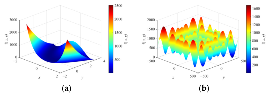
Figure 1.
Three-dimensional surface plot of the basis function: (a) Rosenbrock and (b) Schwefel.
Figure 1.
Three-dimensional surface plot of the basis function: (a) Rosenbrock and (b) Schwefel.
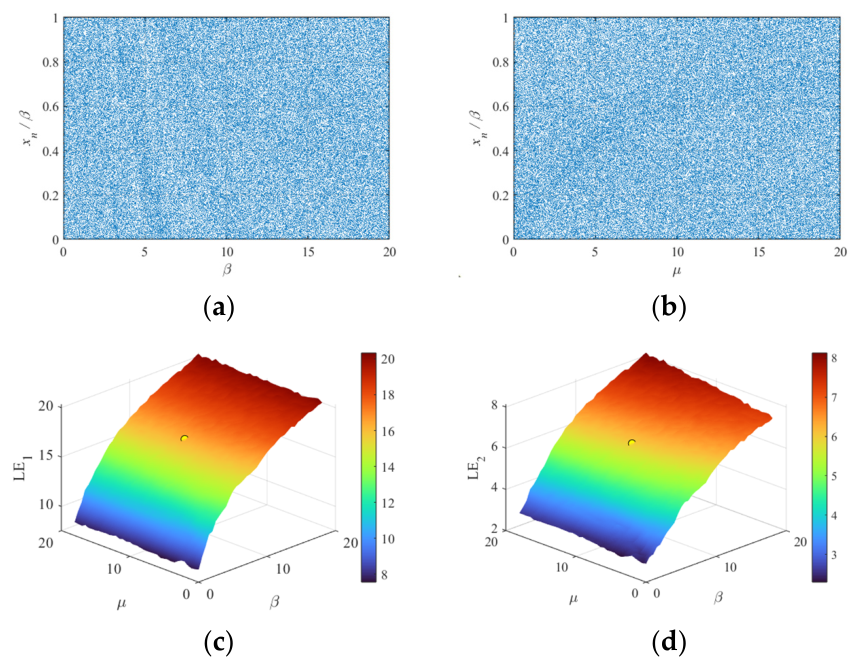
Figure 2.
(a) Normalized bifurcation diagram with respect to β. (b) Normalized bifurcation diagram with respect to μ. (c,d) Three-dimensional Lyapunov-exponent surfaces with respect to μ and β.
Figure 2.
(a) Normalized bifurcation diagram with respect to β. (b) Normalized bifurcation diagram with respect to μ. (c,d) Three-dimensional Lyapunov-exponent surfaces with respect to μ and β.
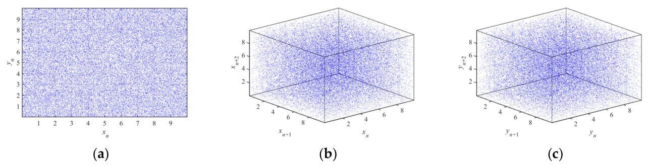
Figure 3.
Initial state (x0, y0) = (0.6, 0.5), parameter a = b = 8, β = 10: (a) phase trajectory of yn relative to xn; (b) relationship between xn+2 relative to xn+1 and xn; (c) relationship between y(n+2) and yn+1.
Figure 3.
Initial state (x0, y0) = (0.6, 0.5), parameter a = b = 8, β = 10: (a) phase trajectory of yn relative to xn; (b) relationship between xn+2 relative to xn+1 and xn; (c) relationship between y(n+2) and yn+1.
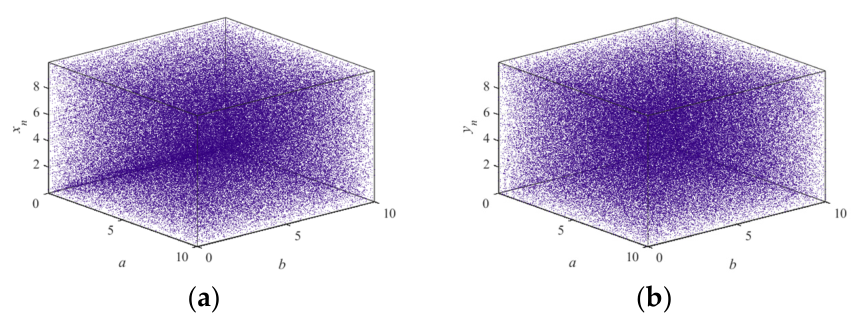
Figure 4.
Initial values (x0, y0) = (0.6, 0.5) and β = 10: bifurcation diagram as control parameters a and b vary: (a) State variable xn; (b) State variable yn.
Figure 4.
Initial values (x0, y0) = (0.6, 0.5) and β = 10: bifurcation diagram as control parameters a and b vary: (a) State variable xn; (b) State variable yn.
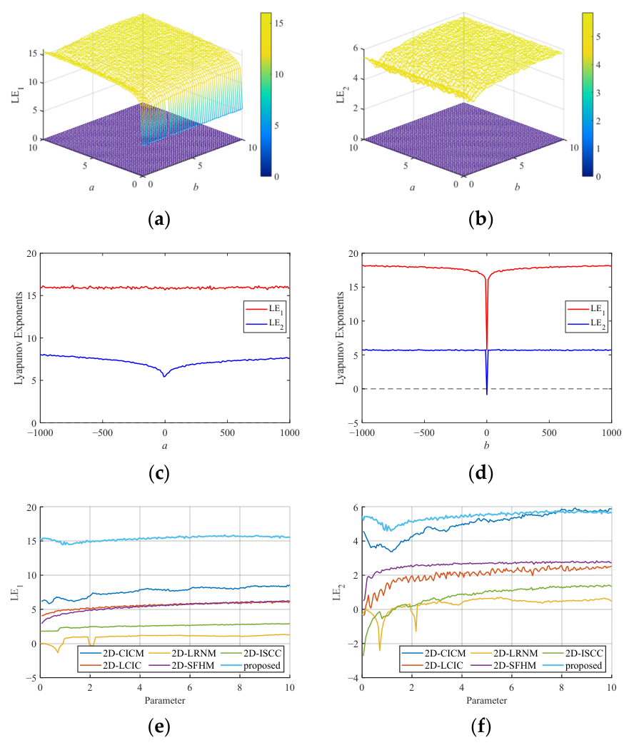
Figure 5.
LE analysis: (a,b) three-dimensional visualization of LE; (c,d) LE analysis across a broader parameter range; (e,f) comparative analysis curves of LE versus control parameters.
Figure 5.
LE analysis: (a,b) three-dimensional visualization of LE; (c,d) LE analysis across a broader parameter range; (e,f) comparative analysis curves of LE versus control parameters.
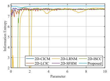
Figure 6.
Comparison of Shannon entropy for sequences generated by different chaotic maps.
Figure 6.
Comparison of Shannon entropy for sequences generated by different chaotic maps.
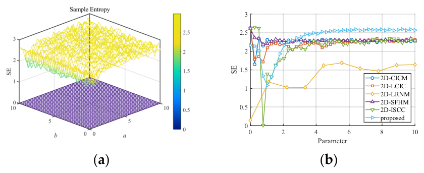
Figure 7.
SE analysis: (a) three-dimensional visualization of SE; (b) comparative analysis curve of SE versus control parameters.
Figure 7.
SE analysis: (a) three-dimensional visualization of SE; (b) comparative analysis curve of SE versus control parameters.
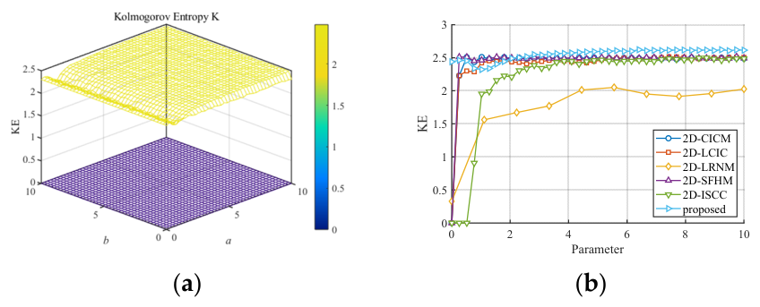
Figure 8.
KE analysis: (a) three-dimensional visualization of KE; (b) comparative analysis curve of KE versus control parameters.
Figure 8.
KE analysis: (a) three-dimensional visualization of KE; (b) comparative analysis curve of KE versus control parameters.
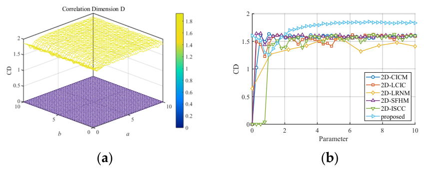
Figure 9.
CD analysis: (a) three-dimensional visualization of CD; (b) comparative analysis curve of CD versus control parameters.
Figure 9.
CD analysis: (a) three-dimensional visualization of CD; (b) comparative analysis curve of CD versus control parameters.
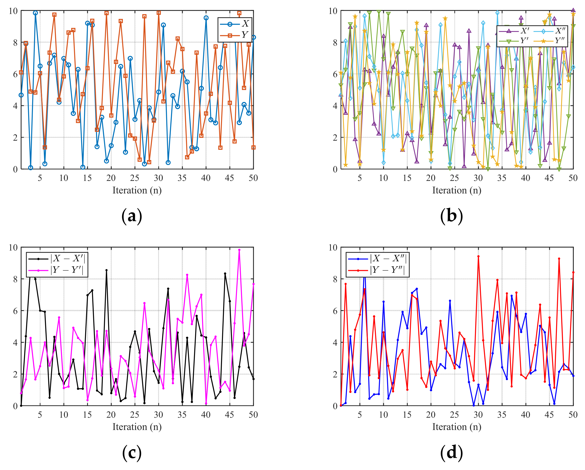
Figure 10.
Sensitivity analysis of the proposed 2D-RS map to initial conditions and control parameters: (a) reference sequences X and Y generated from the original initial conditions; (b) perturbed sequences X′ and Y′ obtained by changing the initial conditions, together with sequences X″ and Y″ obtained by perturbing the control parameters; (c) absolute differences |X−X′| and |Y−Y′| caused by the initial-condition perturbation; (d) absolute differences |X−X″| and |Y−Y″| caused by the control-parameter perturbation.
Figure 10.
Sensitivity analysis of the proposed 2D-RS map to initial conditions and control parameters: (a) reference sequences X and Y generated from the original initial conditions; (b) perturbed sequences X′ and Y′ obtained by changing the initial conditions, together with sequences X″ and Y″ obtained by perturbing the control parameters; (c) absolute differences |X−X′| and |Y−Y′| caused by the initial-condition perturbation; (d) absolute differences |X−X″| and |Y−Y″| caused by the control-parameter perturbation.
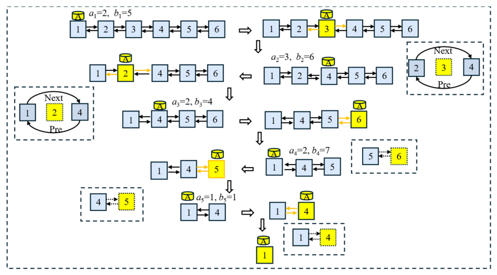
Figure 11.
Schematic diagram of topological permutation.
Figure 11.
Schematic diagram of topological permutation.
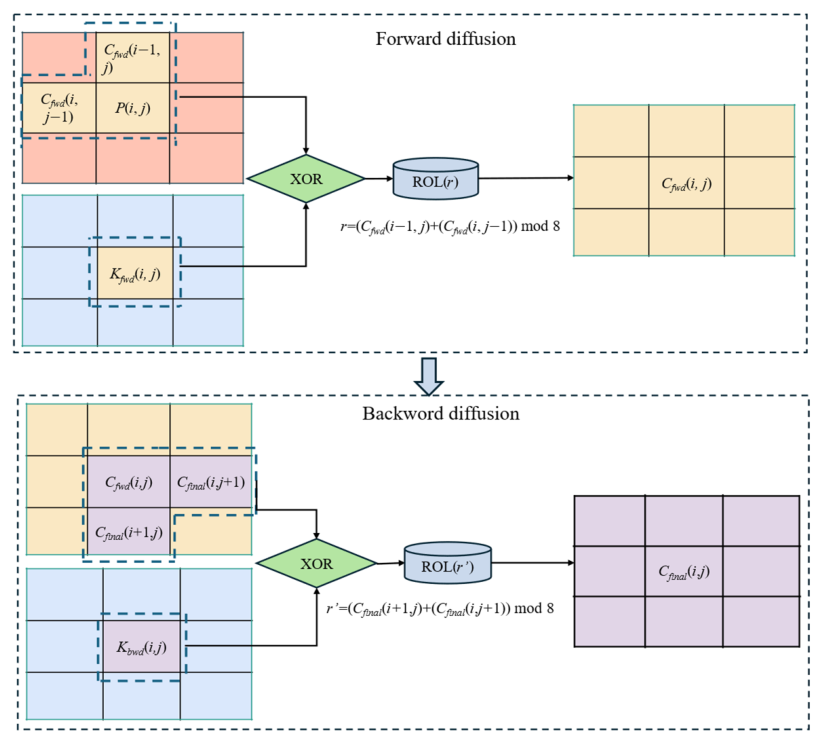
Figure 12.
Schematic diagram of bidirectional diffusion with adaptive dynamic shift.
Figure 12.
Schematic diagram of bidirectional diffusion with adaptive dynamic shift.
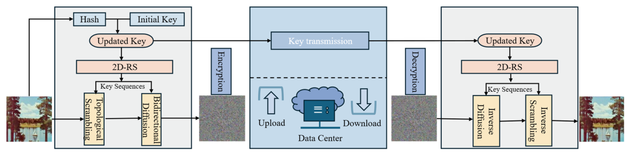
Figure 13.
Overall encryption and decryption flowchart.
Figure 13.
Overall encryption and decryption flowchart.
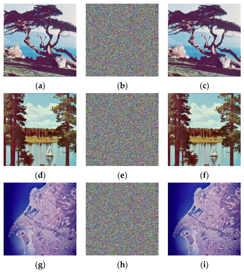
Figure 14.
Encryption and decryption tests: Plain images are (a) 4.1.06, (d) 4.2.06, and (g) 2.2.01; (b), (e), and (h) represent the corresponding cipher images for (a), (d), and (g), respectively; (c), (f), and (i) represent the decrypted and restored images for the aforementioned plain images, respectively.
Figure 14.
Encryption and decryption tests: Plain images are (a) 4.1.06, (d) 4.2.06, and (g) 2.2.01; (b), (e), and (h) represent the corresponding cipher images for (a), (d), and (g), respectively; (c), (f), and (i) represent the decrypted and restored images for the aforementioned plain images, respectively.
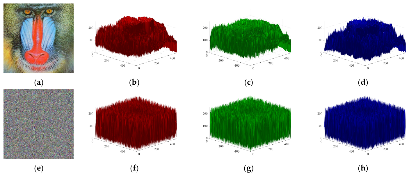
Figure 15.
4.2.03 Histogram analysis of images: (a) 4.2.03; (b) plaintext channel R; (c) plaintext channel G; (d) plaintext channel B; (e) 4.2.03 ciphertext image (f) ciphertext channel R; (g) ciphertext channel G; (h) ciphertext channel B.
Figure 15.
4.2.03 Histogram analysis of images: (a) 4.2.03; (b) plaintext channel R; (c) plaintext channel G; (d) plaintext channel B; (e) 4.2.03 ciphertext image (f) ciphertext channel R; (g) ciphertext channel G; (h) ciphertext channel B.
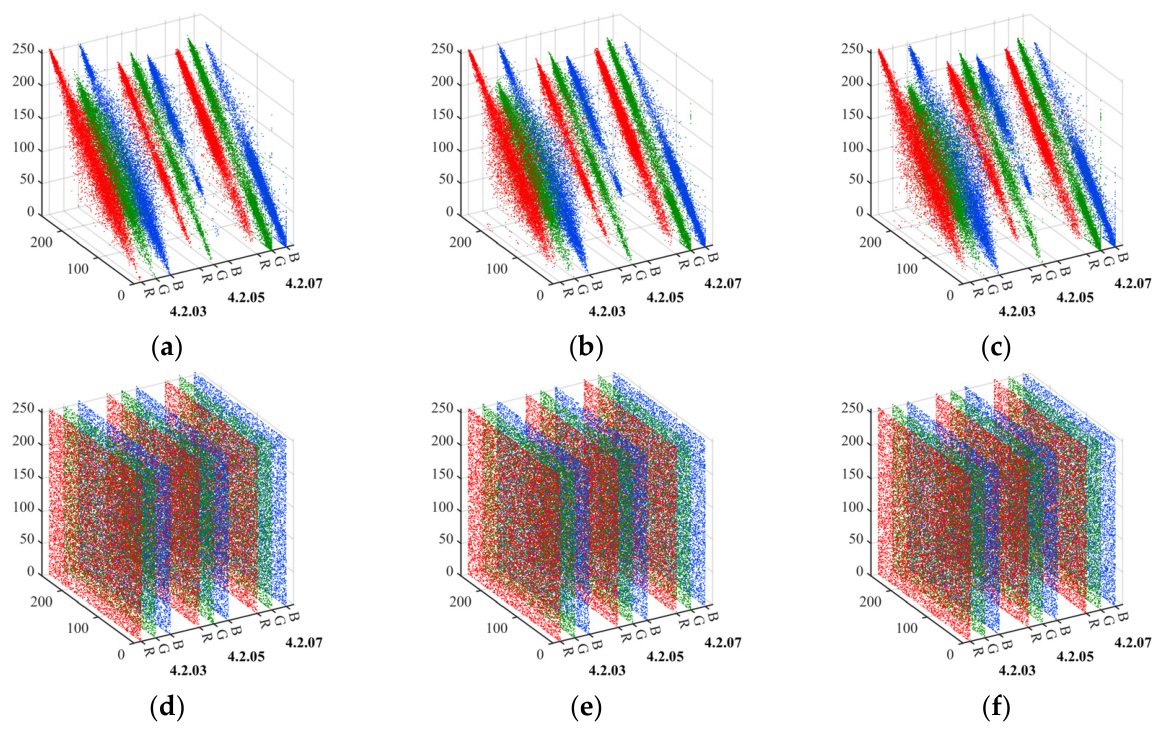
Figure 16.
Image correlation analysis: (a–c) represent the adjacent pixel correlations of the plain image in three directions; (d–f) represent the adjacent pixel correlations of the cipher image in three directions.
Figure 16.
Image correlation analysis: (a–c) represent the adjacent pixel correlations of the plain image in three directions; (d–f) represent the adjacent pixel correlations of the cipher image in three directions.
Figure 17.
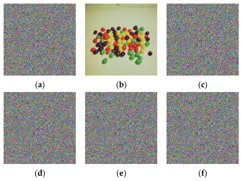
Key sensitivity test results: (a) cipher image encrypted using Key0 keys; (b) recovered image decrypted using Key0 keys; (c–f) images decrypted using Key1, Key2, Key3, and Key4.
Figure 17.
Key sensitivity test results: (a) cipher image encrypted using Key0 keys; (b) recovered image decrypted using Key0 keys; (c–f) images decrypted using Key1, Key2, Key3, and Key4.
Figure 18.
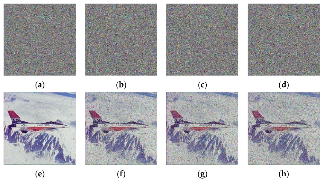
Robustness against attack experimental results: (a) Cipher image with 0.5% salt-and-pepper noise added; (b) Cipher image with 5% salt-and-pepper noise added; (c) cipher image with 6% salt-and-pepper noise added; (d) cipher image with 8% salt-and-pepper noise added; (e) decrypted and restored image corresponding to (a); (f) decrypted and restored image corresponding to (b); (g) decrypted and restored image corresponding to (c); (h) decrypted and restored image corresponding to (d).
Figure 18.
Robustness against attack experimental results: (a) Cipher image with 0.5% salt-and-pepper noise added; (b) Cipher image with 5% salt-and-pepper noise added; (c) cipher image with 6% salt-and-pepper noise added; (d) cipher image with 8% salt-and-pepper noise added; (e) decrypted and restored image corresponding to (a); (f) decrypted and restored image corresponding to (b); (g) decrypted and restored image corresponding to (c); (h) decrypted and restored image corresponding to (d).
Figure 19.
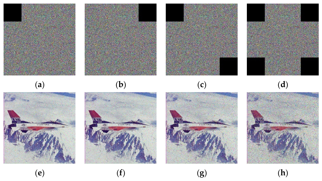
Crop attack experimental results: (a) Cipher image with 128 128 3 pixels missing from the top-left corner; (b) cipher image with 128 128 3 pixels missing from the top-right corner; (c) cipher image with 128 128 3 pixels missing from both the top-left and bottom-right corners; (d) cipher image with 128 128 3 pixels missing from all four corners; (e) decrypted and restored image corresponding to (a); (f) decrypted and restored image corresponding to (b); (g) decrypted and restored image corresponding to (c); (h) decrypted and restored image corresponding to (d).
Figure 19.
Crop attack experimental results: (a) Cipher image with 128 128 3 pixels missing from the top-left corner; (b) cipher image with 128 128 3 pixels missing from the top-right corner; (c) cipher image with 128 128 3 pixels missing from both the top-left and bottom-right corners; (d) cipher image with 128 128 3 pixels missing from all four corners; (e) decrypted and restored image corresponding to (a); (f) decrypted and restored image corresponding to (b); (g) decrypted and restored image corresponding to (c); (h) decrypted and restored image corresponding to (d).
Figure 20.
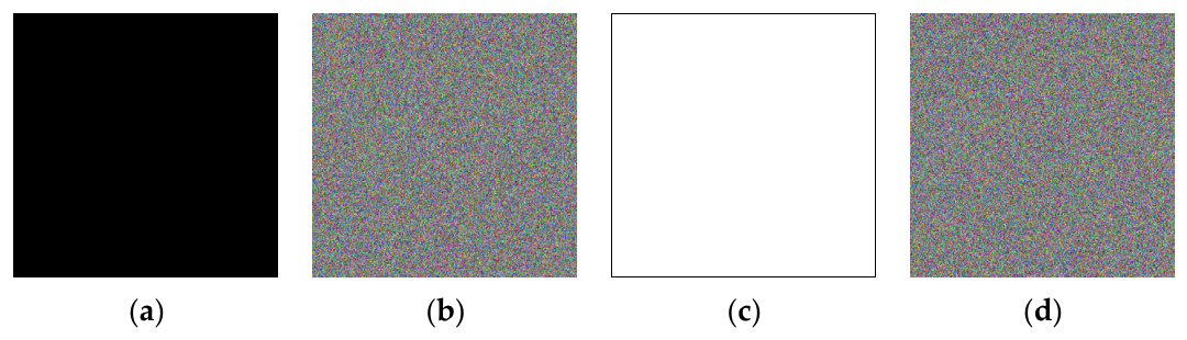
Simulation results for specific images: (a) all-black image; (b) cipher image after encryption of the all-black image; (c) all-white image; (d) cipher image after encryption of the all-white image.
Figure 20.
Simulation results for specific images: (a) all-black image; (b) cipher image after encryption of the all-black image; (c) all-white image; (d) cipher image after encryption of the all-white image.
Table 1.
Existing 2D chaotic maps with control parameters.
Table 1.
Existing 2D chaotic maps with control parameters.
| Reference | Name | F (x, y) | Parameters |
|---|
| [37] | 2D-CICM | | a, b |
| [20] | 2D-LCIC | | a, b |
| [19] | 2D-LRNM | | , , , , |
| [38] | 2D-SHFM | | a, b |
| [20] | 2D-ISCC | | a, b |
Table 2.
NIST test results.
Table 2.
NIST test results.
| No. | Statistical Test | p Value of x | S or F (x) | p Value of y | S or F (y) |
|---|
| 1 | Frequency | 0.2576 | S | 0.2846 | S |
| 2 | Block-frequency | 0.1583 | S | 0.3427 | S |
| 3 | Cumulative sums | 0.7318 | S | 0.4752 | S |
| 4 | Runs | 0.6867 | S | 0.2131 | S |
| 5 | Longest runs of Ones | 0.7385 | S | 0.1165 | S |
| 6 | Rank | 0.0408 | S | 0.2777 | S |
| 7 | Discrete Fourier transform test | 1.0000 | S | 0.4506 | S |
| 8 | Non overlapping template matching | 0.0964 | S | 0.9752 | S |
| 9 | Overlapping template matching | 0.2337 | S | 0.7955 | S |
| 10 | Universal statistical | 0.9748 | S | 0.4622 | S |
| 11 | Approximate entropy | 0.4512 | S | 0.9523 | S |
| 12 | Random excursions | 1.0000 | S | 1.0000 | S |
| 13 | Random excursions variant | 0.1317 | S | 0.3110 | S |
| 14 | Serial | 0.1315 | S | 0.0207 | S |
| 15 | Linear complexity | 0.5308 | S | 0.1842 | S |
Table 3.
Information entropy of cipher images in the R, G, and B individual channels.
Table 3.
Information entropy of cipher images in the R, G, and B individual channels.
| Size | Image | Plain R | Plain G | Plain B | Cipher R | Cipher G | Cipher B |
|---|
| 1024 × 1024 × 3 | 2.2.01 | 7.7575 | 7.3387 | 6.9561 | 7.9998 | 7.9998 | 7.9998 |
| 1024 × 1024 × 3 | 2.2.05 | 7.4445 | 7.2346 | 6.5896 | 7.9998 | 7.9998 | 7.9998 |
| 1024 × 1024 × 3 | 2.2.08 | 7.7229 | 7.5289 | 6.8318 | 7.9998 | 7.9998 | 7.9998 |
| 512 × 512 × 3 | 4.2.03 | 7.7067 | 7.4744 | 7.7522 | 7.9994 | 7.9993 | 7.9993 |
| 512 × 512 × 3 | 4.2.05 | 6.7178 | 6.7990 | 6.2138 | 7.9993 | 7.9993 | 7.9993 |
| 512 × 512 × 3 | 4.2.07 | 7.3388 | 7.4963 | 7.0583 | 7.9993 | 7.9993 | 7.9993 |
| 256 × 256 × 3 | 4.1.05 | 6.4311 | 6.5389 | 6.2320 | 7.9976 | 7.9968 | 7.9974 |
| 256 × 256 × 3 | 4.1.06 | 7.2104 | 7.4136 | 6.9207 | 7.9973 | 7.9976 | 7.9976 |
| 256 × 256 × 3 | 4.1.07 | 5.2626 | 5.6947 | 6.5464 | 7.9972 | 7.9975 | 7.9973 |
Table 4.
Cipher image information entropy comparison analysis across the R, G, and B channels.
Table 4.
Cipher image information entropy comparison analysis across the R, G, and B channels.
| Image | Channel | [25] | [50] | [51] | [52] | Proposed |
|---|
| 4.2.03 | R | 7.9993 | 7.9992 | 7.9993 | - | 7.9994 |
| | G | 7.9992 | 7.9993 | 7.9993 | - | 7.9993 |
| | B | 7.9993 | 7.9992 | 7.9993 | - | 7.9993 |
| 4.2.07 | R | 7.9993 | 7.9991 | 7.9992 | 7.9993 | 7.9993 |
| | G | 7.9994 | 7.9992 | 7.9993 | 7.9993 | 7.9993 |
| | B | 7.9992 | 7.9992 | 7.9993 | 7.9992 | 7.9993 |
Table 5.
Local entropy of cipher images in the R, G, and B individual channels.
Table 5.
Local entropy of cipher images in the R, G, and B individual channels.
| Image | Plain R | Plain G | Plain B | Cipher R | Cipher G | Cipher B |
|---|
| 2.2.01 | 6.1976 | 5.5680 | 5.4120 | 7.9020 | 7.9003 | 7.9027 |
| 2.2.05 | 6.7882 | 6.4635 | 5.7994 | 7.8997 | 7.9047 | 7.9025 |
| 2.2.08 | 6.4940 | 6.1577 | 5.3923 | 7.9028 | 7.9010 | 7.9039 |
| 4.2.03 | 6.5207 | 6.9240 | 6.7512 | 7.9016 | 7.9029 | 7.9009 |
| 4.2.05 | 5.1153 | 5.7048 | 5.1815 | 7.9029 | 7.9067 | 7.9028 |
| 4.2.07 | 6.0375 | 6.0249 | 5.9805 | 7.9029 | 7.9028 | 7.9020 |
| Mean | 6.1922 | 6.1405 | 5.7528 | 7.9020 | 7.9031 | 7.9025 |
Table 6.
Correlation between adjacent pixels in plain images across three directions.
Table 6.
Correlation between adjacent pixels in plain images across three directions.
| Image | Direction | Plain R | Plain G | Plain B | Cipher R | Cipher G | Cipher B |
|---|
| 2.2.01 | Horizontal | 0.926506 | 0.920748 | 0.909147 | 0.003877 | −0.003882 | −0.005246 |
| | Vertical | 0.920383 | 0.914158 | 0.906562 | −0.000479 | 0.002018 | 0.002326 |
| | Diagonal | 0.904060 | 0.891374 | 0.884262 | −0.008652 | 0.005260 | −0.000334 |
| 2.2.05 | Horizontal | 0.938527 | 0.944266 | 0.897832 | −0.006536 | −0.005707 | −0.003392 |
| | Vertical | 0.929513 | 0.924286 | 0.878533 | 0.000296 | 0.004099 | 0.001342 |
| | Diagonal | 0.908868 | 0.915538 | 0.875350 | 0.004142 | −0.003659 | 0.000972 |
| 2.2.08 | Horizontal | 0.922927 | 0.920235 | 0.900228 | 0.003824 | −0.003666 | −0.003271 |
| | Vertical | 0.922631 | 0.912370 | 0.891840 | −0.003303 | 0.000658 | 0.006389 |
| | Diagonal | 0.904331 | 0.895095 | 0.871136 | −0.004262 | 0.004048 | −0.005116 |
| 4.2.03 | Horizontal | 0.920144 | 0.871085 | 0.903918 | −0.000802 | 0.005571 | −0.000525 |
| | Vertical | 0.871106 | 0.753188 | 0.879148 | 0.000281 | −0.000751 | 0.001744 |
| | Diagonal | 0.858287 | 0.744541 | 0.845235 | −0.00057 | 0.000688 | 0.001098 |
| 4.2.05 | Horizontal | 0.974016 | 0.955423 | 0.964890 | 0.001767 | 0.000190 | 0.002774 |
| | Vertical | 0.959348 | 0.964018 | 0.935032 | −0.002039 | −0.006399 | −0.000457 |
| | Diagonal | 0.934451 | 0.938564 | 0.913482 | 0.003709 | −0.000335 | −0.002053 |
| 4.2.07 | Horizontal | 0.965928 | 0.980581 | 0.968250 | −0.002989 | 0.001654 | −0.00064 |
| | Vertical | 0.965683 | 0.980843 | 0.968139 | 0.003457 | 0.000957 | −0.000713 |
| | Diagonal | 0.961562 | 0.965546 | 0.948582 | −0.000334 | −0.000205 | 0.000264 |
| 4.1.06 | Horizontal | 0.957655 | 0.969344 | 0.960901 | 0.002696 | −0.000769 | 0.009187 |
| | Vertical | 0.936754 | 0.942640 | 0.943474 | 0.002895 | −0.007363 | 0.004369 |
| | Diagonal | 0.917956 | 0.931956 | 0.927970 | 0.003832 | −0.002387 | −0.005014 |
| 4.1.07 | Horizontal | 0.975149 | 0.973212 | 0.988038 | 0.000313 | −0.008739 | −0.005658 |
| | Vertical | 0.978002 | 0.980417 | 0.988020 | 0.001538 | 0.006290 | 0.001060 |
| | Diagonal | 0.958514 | 0.960670 | 0.980307 | −0.004597 | 0.000893 | 0.000733 |
| 4.1.05 | Horizontal | 0.965973 | 0.982242 | 0.981483 | −0.000318 | −0.001982 | −0.001167 |
| | Vertical | 0.935828 | 0.952571 | 0.974160 | −0.004442 | −0.001128 | 0.002311 |
| | Diagonal | 0.914885 | 0.933288 | 0.963357 | 0.001606 | −0.003309 | 0.007272 |
Table 7.
Correlation analysis of cipher images across the R, G, and B channels.
Table 7.
Correlation analysis of cipher images across the R, G, and B channels.
| Images | Dir | Channel | [25] | [50] | [51] | [52] | Proposed |
|---|
| 4.2.03 | H | R | −0.0012 | −0.0077 | −0.00006 | - | −0.0008 |
| | | G | 0.0005 | 0.0038 | 0.0005 | - | 0.005571 |
| | | B | −0.0001 | −0.008 | −0.0003 | - | −0.00053 |
| | V | R | 0.0003 | 0.0056 | 0.0005 | - | 0.000281 |
| | | G | 0.0006 | −0.0029 | 0.0006 | - | −0.00075 |
| | | B | −0.0003 | −0.0028 | −0.00003 | - | 0.001744 |
| | D | R | 0.0048 | 0.0016 | −0.0013 | - | −0.00057 |
| | | G | −0.0062 | −0.0017 | −0.0005 | - | 0.000688 |
| | | B | −0.0076 | 0.0001 | 0.0008 | - | 0.001098 |
| 4.2.07 | H | R | 0.0067 | 0.0057 | 0.0014 | 0. 0027 | −0.00299 |
| | | G | −0.0062 | −0.0098 | 0.0008 | 0.0017 | 0.001654 |
| | | B | 0.0048 | 0.0068 | 0.0012 | 0.0014 | −0.00064 |
| | V | R | 0.0036 | 0.0036 | 0.0025 | 0.0016 | 0.003457 |
| | | G | 0.0037 | 0.0037 | 0.0019 | 0.0001 | 0.000957 |
| | | B | 0.0043 | 0.0043 | −0.0003 | 0.0005 | −0.00071 |
| | D | R | −0.0073 | −0.0058 | −0.00009 | 0.0015 | −0.00033 |
| | | G | −0.0040 | −0.0012 | −0.0034 | 0.0004 | −0.00021 |
| | | B | 0.0041 | −0.0022 | 0.0041 | 0.0003 | 0.000264 |
Table 8.
NPCR (%) and UACI (%) metrics for cipher images.
Table 8.
NPCR (%) and UACI (%) metrics for cipher images.
| Image | NPCR | UACI |
|---|
| 2.2.01 | 99.6083 | 33.4634 |
| 2.2.05 | 99.6061 | 33.4731 |
| 2.2.08 | 99.6132 | 33.4472 |
| 4.2.03 | 99.6157 | 33.4985 |
| 4.2.05 | 99.6001 | 33.4655 |
| 4.2.07 | 99.6175 | 33.4347 |
| 4.1.05 | 99.5860 | 33.4492 |
| 4.1.06 | 99.6109 | 33.4908 |
| 4.1.07 | 99.6109 | 33.4923 |
| Average | 99.6076 | 33.4683 |
Table 9.
Encryption time (seconds) and encryption throughput for different sizes.
Table 9.
Encryption time (seconds) and encryption throughput for different sizes.
| Reference | Size | EH | ETH |
|---|
| [25] | 512 × 512 × 3 | 0.8569 | 0.8752 |
| [50] | 256 × 256 × 3 | 0.4262 | - |
| | 512 × 512 × 3 | 0.9220 | - |
| [51] | 256 × 256 | 0.0794 | 0.7872 |
| | 512 × 512 × 3 | 0.9447 | 0.2646 |
| [52] | 256 × 256 × 3 | 0.077 | - |
| | 512 × 512 × 3 | 0.281 | - |
| Proposed | 256 × 256 | 0.1792 | 0.3488 |
| | 256 × 256 × 3 | 0.4789 | 0.3915 |
| | 512 × 512 × 3 | 1.7329 | 0.4328 |