1.1. Axiomatic Basis: Minimal Architecture
In a background-independent theory, there is no external clock and no pre-existing global stage on which local observables are simply placed. Locality must therefore be defined operationally from the finite record accessible to an observer. The causal diamond provides the minimal covariant laboratory for this local inference [
2], defined by two timelike-separated events and independent of global backgrounds. Within this region, diffeomorphism and Gauss-law constraints obstruct naive bulk factorization, so subregion data must be tied to a closed boundary interface, the waist
. Holographic bounds require finite information capacity. Modular flow then supplies the intrinsic clock, boundary completion defines the measurable algebra, and finite resolution fixes the common operator content used to compare
with
.
Consequently, we formulate quantum gravity as local statistical inference in a background-independent, finite-resolution setting, bypassing the need for a preferred lattice or pre-defined field content.
The axioms P1–P7 define the operational domain for subsystems, clocks and regulated observables. Topology, transport and spin structure then specify the minimal boundary sector, while constitutive relations calibrate its microscopic capacity to macroscopic gravity. Phenomenological results follow as outputs of this combined architecture. The axioms are organized under three architectural principles:
Locality is defined operationally by the minimal covariant unit: a finite causal diamond [
2]. This geometry fixes the boundary interface where subsystem-defining information must reside [
11].
P1 (Non-factorization). The diffeomorphism-invariant physical Hilbert space does not factorize across spatial subregions (
). Constraint relations tie interior data to boundary charges and fluxes, requiring explicit boundary data (edge modes) to define a well-specified subregion algebra [
11,
12,
13,
14].
P2 (Causal Diamonds). A finite experiment is a closed query–response loop between two timelike-separated events
p and
q. A causal diamond
[
2] covariantly defines an observer’s operational workspace. We restrict to the minimal simply connected sector: a maximal spatial slice of topology
with a single closed waist
. This is the minimal local topology supporting a closed boundary completion (P3); nontrivial topologies require extra gluing data and lie outside the present analysis.
P3 (Boundary Completion). Since the physical Hilbert space does not factorize (P1), a well-defined subregion algebra
requires boundary completion. States are positive, normalized functionals on
. This interface acts as a coherency screen at the diamond waist
, reconciling overlapping past and future boundary data into a unified record. We adopt a boundary-completed algebra whose finite-resolution center
carries the gluing and charge labels needed to encode Gauss-law constraints. This ensures that
and
live on identical operator content and define a common variational domain [
11,
13,
15].
Finite capacity prevents unbounded boundary information density [
16,
17]. In the small-diamond KMS regime, modular flow supplies the intrinsic local clock [
4,
5,
18].
P4 (Modular Locality). In the local Rindler regime, the vacuum restricted to
is approximately KMS with respect to a geometric modular flow. This applies in the small-diamond regime, where the diamond size is intermediate between the resolution limit and the local curvature radius. The modular Hamiltonian is well-approximated by the local boost generator, fixing KMS periodicity
[
4,
5].
Corollary (Canonical History Manifold). In the minimal simply connected sector, the two spatial domains associated with the causal-diamond halves glue across the waist as . The KMS condition evaluates local response on a compact Euclidean modular cycle . The spectral trace is therefore represented on , the minimal compact history manifold for this sector.
P5 (Finite Resolution). Defining a local subsystem requires finite resolution to ensure a stable restriction to
and a bounded mode density at the interface. Since an algebraic restriction alone cannot fix the physical bandwidth, a proper-distance cutoff
is introduced via a stretched screen in the local Rindler region. This finite-capacity regulator guarantees that
and
admit a well-defined relative-entropy comparison, consistent with holographic bounds [
16,
19,
20].
Corollary (Monotone Spectral Suppression). Relative entropy is monotone under the restriction of the accessible algebra (P3), while finite resolution imposes a strict limit on the information capacity per pixel (P5). In the resolved quasi-local regime, the infrared expansion is therefore organized in terms of intensive response densities and irrelevant corrections suppressed by powers of . Extensive macroscopic quantities may grow with the total number of pixels, but the distinguishability available to each pixel remains bounded by the finite-capacity algebra.
Non-factorization (P1) and boundary completion (P3) place charge labels on the boundary, represented here as discrete topological sectors [
21]. Finite resolution supplies an isotropic transport layer for local excitations [
22]. Near the sub-resolution tips, smooth modular flow must be routed through discrete boundary updates; the resulting digitization cost is the bottleneck that limits phase-coherent capacity.
P6 (Gauge Topology). Boundary charge sectors are encoded by topological current data compatible with non-factorization (P1) and closed algebraic gluing (P3). During one modular cycle, the causal-diamond waist sweeps out the closed boundary history
, whose current response is represented by a Chern–Simons functional [
21]. With the trace normalization fixed, large gauge transformations of compact simple groups shift this functional by integer multiples of
; path-integral phase invariance, therefore, requires
[
23]. Gauss law makes interior flux end on the spatial
interface as representation-carrying punctures. These punctures generate surface states described by Wess–Zumino–Witten conformal blocks, equivalently chiral data organized by the affine Kac–Moody algebra at level
k [
24]. Retaining sectors compatible with KMS periodicity, large-gauge invariance, and anomaly inflow, this integer level fixes the boundary-current normalization entering the matching-scale inverse gauge coupling.
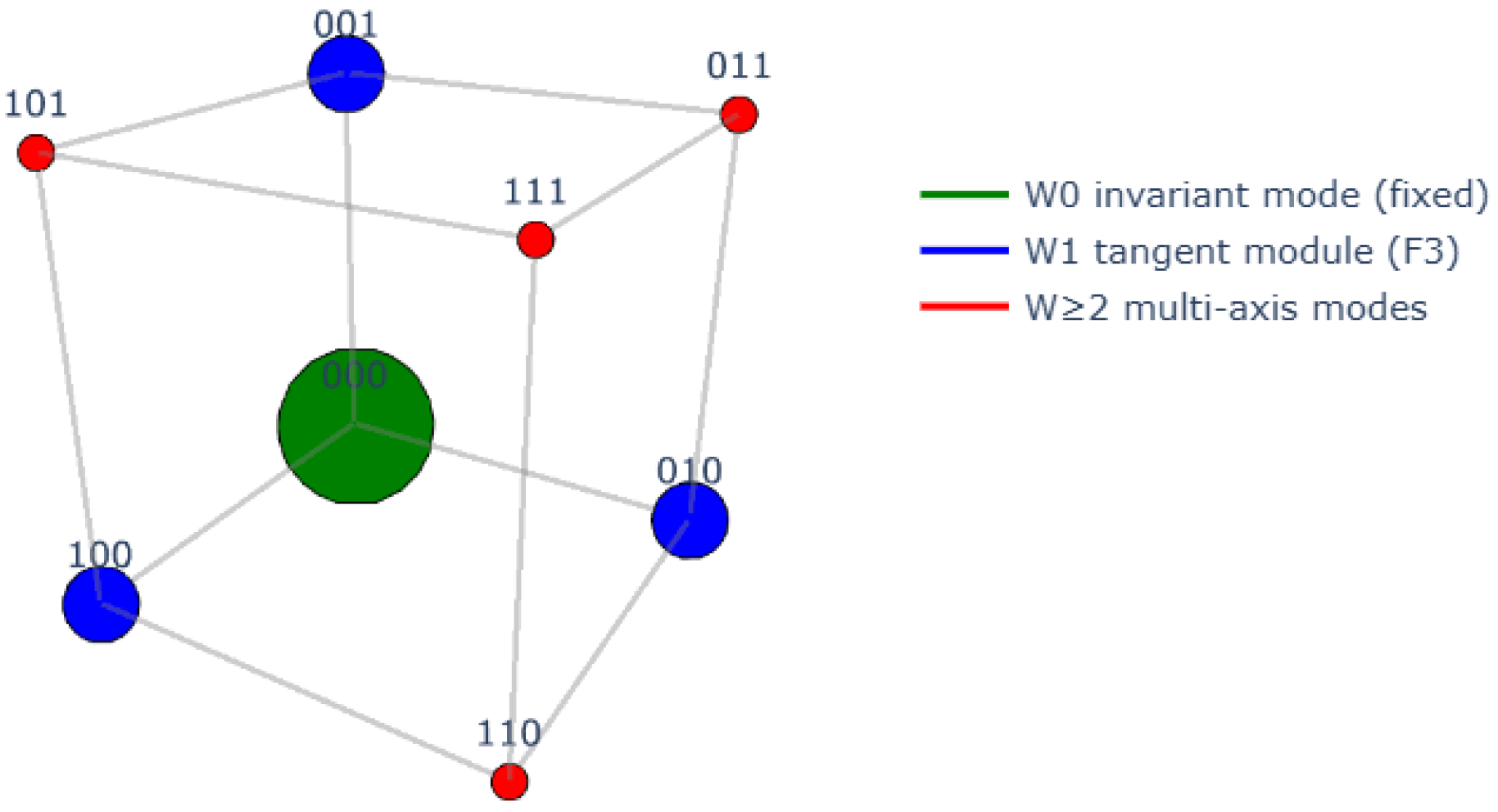
P7 (Discrete Isotropic Transport). A finite-resolution boundary architecture requires a local transport layer that is isotropic after modular averaging, inversion-symmetric, and closed under frame transport. Modular closure requires that after a period, local excitations return to their initial states up to a minimal grading, lacking spurious phases or directional bias. Inversion symmetry pairs every transport direction with its opposite. The absence of directional bias requires the modularly averaged transport to be isotropic, so the second moment of the local step distribution is proportional to the identity. For three equal-length antipodal pairs with equal weights, this condition forces orthonormality, fixing the minimal transport layer to the signed basis , octahedral coordination , and the step rule. This closure requires lifting to its double cover , introducing a minimal grading, and thereby supporting local spinors. Since finite resolution (P5) sets the only intrinsic scale, we select a massless continuum transport operator that recovers local conformal covariance, removing curvature-coupling ambiguities.
Corollary (Resolved Modular Interval and Lorentz Covariance). The cutoff is placed at fixed proper distance from the causal-diamond waist. Because the diamond is defined by light rays, this local placement introduces no preferred global frame. With local Rindler scaling , the unresolved neighborhoods of the modular tips are excised, giving . The canonical screen placement sets in modular units. Nearby choices of rescale only the universal modular-window factor; the normalized coupling ratios remain fixed by the integer boundary-current levels. The discrete transport layer is confined to the boundary completion near the excised tips. Below , the resolved interior is described by continuum fields on a smooth manifold; the leading EFT is locally Lorentz invariant, with regulator artifacts appearing only through irrelevant operators suppressed by powers of .
Corollary (Minimal Regge-Transport Construction). Near the spacetime tips , the transverse cross-section falls below the resolution length , forcing smooth -isotropic modular flow to digitize onto the discrete transport layer. Here, an equal-weight signed router maps angular convergence onto an octahedral triangulation of the screen. At each of the six octahedral vertices, four equilateral triangular sectors meet; their angle sum is , giving a deficit relative to the flat value . The total deficit is therefore , matching the Gaussian-curvature integral of the closed waist (equivalently in scalar-curvature convention).
Corollary (Tip Defect Parameter ). Routing continuous modular flow through the sub-resolution tips incurs an irreducible digitization overhead, encoded by the dimensionless boundary impedance . By P5, the resolved waist is a closed finite transport graph. Euler closure requires a net positive coordination deficit. In the selected minimal inversion-symmetric sector, this closure is realized by the octahedral router with three antipodal transport-axis pairs, . At each of the six octahedral poles, four equilateral triangular sectors meet. The Regge angular deficit is , so the normalized local defect fraction is . The six poles sum to , giving the Gaussian-curvature closure of the sphere. Operationally, when a minimal unresolved update reaches a tip, isotropy forbids assigning it to a preferred transport axis. Its scalar effect is therefore distributed equally over the three independent axes, giving the spatial factor . The remaining normalization comes from the intrinsic modular clock; the modular automorphism of the boundary algebra generates a KMS orbit with Euclidean period . Thus, the per-tip leakage is the one-axis defect fraction averaged over one complete modular cycle: . A full causal-diamond modular cycle crosses both tips p and q, so the cycle-integrated leakage is .
Corollary (Transport-Orientation Redundancy ). The octahedral router contains three antipodal axis pairs,
. Independent reversal of each orientation label generates
; hence,
. These reversals act as equivalent sign conventions rather than propagating degrees of freedom. Under open modular evolution, they coarse-grain into commuting subalgebras (
Section 2).
Corollary (Pixel). At finite resolution, a pixel represents a single resolvable algebraic patch on the boundary, defined by the triple and represented by a node in the mesh. The local algebra acts on the internal fiber , while the transport operator D provides the nearest-neighbor connectivity routing data between adjacent nodes.
Corollary (Quantized Holographic Capacity). Octahedral transport admits compatible uniform subdivision by edge bisection. After n bisections, the number of resolved boundary patches scales as . The leading exponential growth is two-dimensional and area-like, while the invariant term continuously records the Euler closure of the sphere. This realizes the boundary as a holographic area-scaling structure.
The axioms operate hierarchically. Axioms P1–P3 define the subsystem: a causal diamond completed by boundary data on a closed waist. Axioms P4–P5 supply the intrinsic modular clock and finite physical bandwidth. Axioms P6–P7 establish the minimal topological currents and isotropic transport required for gauge and spinorial data. Once the minimal sector is specified (one-tick resolution, octahedral transport, spin-twist, canonical normalizations) the subsequent structures, including , N, , , the Hessian blocks and the matching-scale EFT coefficients, arise as constrained outputs (rather than free continuous parameters).
1.2. Boundary Architecture, Resolution and Connectivity
A causal diamond
(P2) is bounded by two null hypersurfaces (future- and past-directed light-sheets) generated by null rays from
p and
q [
2]. Their intersection defines a distinguished spacelike waist 2-sphere
, the maximal-area cross-section of the diamond. This waist serves as the local Rindler cut for the small-diamond description: it is the canonical interface on which a local subregion algebra can be completed when
does not factorize (P1–P3) [
11,
13]. This construction is purely local and does not rely on AdS asymptotics or an AdS/CFT embedding.
Finite resolution (P5) pixelizes the diamond waist:
operates as a finite set of distinguishable boundary patches (pixels) at resolution
; sub-
structures are operationally aliased [
19]. Finite resolution is implemented by replacing the idealized null interface, in the local Rindler neighborhood of the waist, with a stretched screen placed at fixed proper distance
from the cut [
25]. This screen is part of the definition of
: it fixes which edge observables are operationally available and, hence, fixes the common operator content on which both
and the reference family
are defined (P3).
Operationally, the null generators of the diamond act as update channels: the screen registers traversing excitations as discrete arrival events, supplying the raw record compared against . The octahedral mesh on the waist represents this boundary sector, not a discretized bulk spacetime. The system is defined by graph adjacency, local transport rules and internal node labels.
In the local Rindler regime (P4), the local proper time at the screen scales as
[
5]. Identifying the minimal resolvable proper time with the screen resolution (
) defines the canonical matching protocol
. Nearby choices of
rescale the kinematic integration window uniformly across all gauge sectors. Thus the absolute normalization is tied to the canonical screen placement, while the integer-level ratios of inverse couplings remain topologically protected and depend only on the levels
.
Transport across pixels follows the minimal router (P7), implemented in local orthonormal frames of the three-dimensional spatial slice and represented patchwise on the
waist. A global tangent-frame description on
is obstructed, so the screen description is local [
26,
27]. The induced
step metric approximates the smooth
isotropic limit; the mismatch becomes relevant near the diamond tips where the cross-section becomes sub-resolution, producing an irreducible digitization overhead, parametrized by
[
28].
The interface is the waist . Boundary completion represents interior conserved charge sectors as boundary flux labels (P1, P3, P6), reflecting the Gauss-law requirement that charges in a region be encoded by flux through its boundary. The normalization of the local vector response is therefore tied to the surface geometry. We use the standard infrared convention . In the present boundary formulation, this convention aligns the gauge coupling with the flux normalization through the closed interface.
1.3. Topological Budget: Effective Internal Degeneracy
The diamond waist serves as the observer’s operational horizon: an instantaneous coherency screen formed by the unique spatial intersection where the past light cone (incoming data from initiation p) meets the future light cone (outgoing responses registered at q). To determine the effective internal degeneracy N of this screen, we define the baseline vacuum capacity functional from the topological, tip and spin structures specified by P2–P7. This functional counts internal response depth per resolved boundary patch, not the number of patches. The modular periodicity gives this functional its KMS interpretation, while finite resolution makes it a capacity measure for the boundary completion. Physical area enters separately through the number of surface patches (). Retaining only dimensionless, scale-free terms, separates macroscopic area from internal edge capacity.
Boundary completion requires a topologically closed interface to satisfy the Gauss-law for interior charge encoding. On the simply connected waist , the available additive, scale-free local curvature integral is the Euler term. We use the scalar-curvature convention, so the Gauss–Bonnet integral gives rather than the Gaussian-curvature value .
The Gauss–Bonnet theorem [
29,
30] supplies the unique dimensionless closed-waist curvature invariant entering the capacity functional. In the minimal sector, we denote its logarithmic capacity contribution by:
Here is not a thermodynamic entropy and the Gauss–Bonnet theorem does not by itself count microscopic states. It is a dimensionless logarithmic capacity contribution assigned by the finite-resolution boundary architecture. More generally, one could write . The selected minimal sector uses the no-extra-parameter normalization , giving . Choosing would introduce an additional boundary-capacity parameter and define a different matching sector.
Finite representatives must preserve this closed topology (). Open geometries are excluded to avoid unconstrained boundary-circle data.
By Gauss–Bonnet, the waist radius drops out: curvature and area scale inversely, leaving only the Euler invariant. The
term is therefore not an area entropy, but the baseline information capacity of the closed surface. It acts as a fixed topological overhead for boundary charges and edge modes, similar to topological entanglement entropy [
11,
13,
31,
32]. This scale-independent structure ensures the algebraic gluing required by non-factorization and boundary completion (P1–P3).
A hemisphere is excluded in the selected sector because its boundary circle would require additional edge data and would no longer represent the closed Gauss-law interface used for the capacity functional. Geometric, scale-dependent or multiply bounded choices define different capacity functionals outside the chosen architecture.
The transport input for the capacity budget is the octahedral router () (P7). A closed modular cycle must treat each local direction and its reverse symmetrically; otherwise, the transport layer would introduce directional bias. Tetrahedral coordination () lacks antipodal pairs and fails inversion symmetry, while an icosahedral router () adds transport directions beyond those needed to span three dimensions. Within the signed, inversion-symmetric router class, the minimal spanning set is . Thus is the minimal transport architecture used in the capacity count.
At the diamond tips , the transverse cross-section falls below the resolution length (P5). Smooth modular flow can no longer be represented as a continuous transverse field there. It must be recorded as a discrete boundary update on the transport layer selected by P7.
Physically, the tip is the place where a smooth isotropic flow is forced through a finite, graph-local router. The minimal inversion-symmetric router has three antipodal transport-axis pairs, . Since no axis is preferred, one unresolved tip update must be distributed equally over the three independent axes, yielding the spatial factor . The same factor appears geometrically in the octahedral Regge construction. A closed triangular transport mesh cannot form a sphere without positive curvature defects. In the octahedral seed graph, four equilateral triangular sectors meet at each pole, so the angular deficit is . The normalized missing angular fraction is, therefore, . The six poles sum to , ensuring the sphere curvature closure.
The remaining normalization comes from the intrinsic modular clock; the modular automorphism of the boundary algebra generates a KMS orbit with Euclidean period
. Expressing the per-tip defect as a leakage rate over one full modular cycle gives:
A complete causal-diamond modular cycle crosses both tips p and q, so the cycle-integrated leakage is . This is not an arbitrary normalization. It is the finite-resolution impedance of the diamond tips: the cost of routing smooth modular flow through a closed, isotropic, discrete boundary graph.
The same tip impedance controls coherent tensor participation below and the open-system leakage developed in
Section 2.
The discrete transport structure (P7) must close under frame transport. This requires lifting local rotations from to , thereby supporting local spinors. On the boundary algebra, this lift appears as a grading on closed modular loops.
The contribution counted here is not the Hilbert-space dimension of a local spin- fiber, which belongs to the matter transport sector. The capacity term instead counts the minimal topological wiring required for the boundary algebra to support the spin-parity holonomy associated with this grading. Intuitively, the spinor and the twist count different things. The spinor is the object being transported; the twist is the boundary gluing rule that makes this transport globally consistent.
In the selected minimal non-Abelian edge sector, this wiring is represented by an Ising/Majorana twist defect
[
33], whose fusion rule
implies
and therefore
. Physically, two such boundary twists fuse into an ordinary binary fermion-parity channel. A single twist therefore contributes an irreducible half-bit to the logarithmic capacity budget:
.
Choosing would count the local spinor representation rather than the boundary topological twist, thereby double-counting spinorial degrees of freedom already carried by the local matter sector. The contribution supplies only the minimal boundary spin-parity grading required to close the finite-resolution algebra; it does not introduce a propagating bulk anyon in dimensions.
In summary, the capacity contribution follows this topological hierarchy:
These three contributions arise from independent requirements: closed algebraic gluing, modular-cycle closure and spinorial lift. In this product configuration, their associated state spaces factorize, so their logarithmic capacities add, yielding the total vacuum capacity per pixel:
Because
is dimensionless and additive, it has the form of a logarithmic capacity. As in statistical mechanics and holographic entropy, where
encodes effective state multiplicity, exponentiation converts this capacity budget into a multiplicative response capacity [
16,
34,
35]. We therefore define the effective channel multiplicity of the selected boundary sector by
:
As an exponentiated effective capacity rather than a microscopic Hilbert-space dimension, N need not be an integer. It quantifies the intensive internal response capacity assigned to each patch on the boundary algebra. Confined strictly to the boundary completion, this multiplicity introduces no additional propagating bulk fields.
1.4. Constitutive Relation (Coherent Participation)
With the total internal capacity N fixed by the boundary architecture, gravitational stiffness arises only from the phase-coherent tensor subset that survives a full modular cycle. Channels that lose their quantum phase at the geometric tips thermalize into entropy, leaving only the protected fraction to sustain macroscopic geometric stress.
This coherent participation fraction is fixed below by the tip impedance , allowing us to calibrate the resolution scale using the measured Newton’s constant. Extensive scaling follows naturally from thermodynamic and holographic constraints (P4, P5). We use the reduced Planck mass throughout, so that the Einstein–Hilbert term is normalized as .
Let
denote the modular-cycle coherent projector on the resolved boundary channel space. The elementary tip impedance fixes the normalized coherent fraction:
Equivalently, and .
Geometrically, the causal-diamond tips manifest as the fundamental defects of the resolved region (P5). This assigns two algebraic roles: an additive capacity weight in the logarithmic budget and a multiplicative coherent participation fraction in the tensor response. For both, is structurally fixed by clock and transport normalizations (P4, P7).
N represents a vast set of parallel quantum information channels available to the tensor response. In the linear regime, coherent channels decouple quadratically, so their effective stiffnesses add in the macroscopic Hessian [
36,
37]. Normalizing each active channel by the substrate scale
gives the macroscopic tensor stiffness:
This relation is a dimensional calibration, not a prediction of Newton’s constant. The boundary architecture first determines the dimensionless coherent stiffness depth . The observed value of G is then used exactly once to assign the physical scale , setting the units, while and the emergent tensor structure are fixed independently. This logic is therefore structurally non-circular: dimensionless observables, such as tensor-response sum rules, probe the emergent structure directly rather than rederiving G.
Within this calibrated description,
is not introduced as an independent microscopic resolution scale, but rather as the observed macroscopic stiffness assigned to the coherent effective channel capacity. This stiffness additivity aligns with spectral and induced-gravity viewpoints, where effective couplings are controlled by mode counting, and with species-bound logic, where gravitational strength is diluted by the number of active degrees of freedom [
37,
38].
Within the selected minimal sector, the numerical structure is rigid: the closed-waist capacity weight, the tip impedance, the spin-twist sector, the one-tick modular resolution, and the signed three-axis transport architecture fix N and . These inputs are not continuous parameters. Changing any of them shifts the theory to a different boundary sector or matching convention.
1.5. Numerical Calibration
We now calibrate the resolution scale
using the measured Newton’s constant, expressed through the reduced Planck mass
. With the capacity functional above,
. Solving
for the resolution scale gives:
represents the physical resolution limit of the algebra (sharp focus) where the EFT problem is well-posed: gravitational stiffness, gauge couplings and mass gaps enter as matching data, and in quantized sectors some conditions reduce to closed-form constraints (
Section 3). This calibrated matching scale lies in the intermediate range often associated with high-scale seesaw models and plateau-inflation phenomenology [
39,
40].
In reduced-Planck units, the inverse stiffness scale is . Thus acts as the fundamental resolution limit, while emerges strictly as the collective tensor stiffness of the boundary, eliminating the singular continuum artifact.
Finite resolution (P5) bounds the local excitation capacity of a single boundary pixel. The internal multiplicity N includes the spin-twist factor , which supplies the minimal spin-parity grading. Because this edge twist is not an addressable scalar channel, the saturation estimate uses the non-twist channel count .
With
fixed by the Newton calibration, the single-pixel activation scale is
. More generally, a local scalar operator with
q fermionic legs is governed by a single-pixel saturation cap
. Mass deformations on the boundary-completed algebra must be closed gauge-invariant scalar operators. A hypothetical single-leg insertion (
) is therefore inadmissible. Higher-valence scalar operators (
) further lower the cap, corresponding to higher-dimensional EFT deformations. The leading admissible mass deformation is instead the gauge-invariant bilinear
, fixing
:
The resulting upper bound lies close to the observed top-quark mass (). This proximity serves as a heuristic consistency check of the single-pixel saturation cap, not a mass prediction.
We verify that this calibration preserves the Bekenstein–Hawking entropy structure [
34,
41,
42]. For a horizon of area
A, the standard entropy (in natural units) is
. Substituting
, we obtain:
where
counts the resolved boundary pixels on a waist of area
A. The entropy therefore factors into a geometric pixel count and a coherent internal depth. The two quantities play different roles:
is the per-pixel logarithmic capacity defining
, whereas
is the area-extensive entropy obtained by summing the effective tensor-response depth
over all pixels.
Converting to bits and taking gives bits. This reproduces the standard Bekenstein–Hawking area law and the familiar cosmic entropy scale, providing a consistency check of the calibration.
The result follows algebraically from the constitutive relation . It shows that the standard horizon entropy can be represented as a resolved pixel count multiplied by an effective tensor-response depth. Channel multiplicity supplies the required information density without shrinking the pixel size to , recovering the Bekenstein–Hawking scaling natively at the finite resolution scale . Within this framework, is the physical regulator, while the reduced Planck scale is the collective stiffness scale.