Transfer Learning for Moderate–Dimensional Ridge-Regularized Robust Linear Regression

Abstract

This paper studies transfer learning for ridge-regularized robust linear regression in the moderate–dimensional regime, where the number of predictors is of the same order as the sample size and the regression coefficients are not assumed to be sparse. We propose Trans-RR, which combines a robust ridge estimator from a source study with a robust ridge correction based on the target study. Under mild assumptions, we characterize the asymptotic estimation error of the proposed estimator and show that leveraging source data can substantially improve estimation accuracy relative to the traditional single-study ridge-regularized robust estimator. To guard against negative transfer when the source study is not sufficiently informative, we further propose an adaptive aggregation of Trans-RR with the single-task estimator that selects the mixing weight by cross-validation. Simulation studies and a real-data analysis support the theory and illustrate the transition between positive and negative transfer as the discrepancy between the source and target studies varies.

1. Introduction

Modern statistical analyses often involve several related datasets collected from different studies, populations, or experiments. A basic question is how to use these datasets together to improve prediction and estimation for a study of interest. Transfer learning addresses this question by borrowing useful information from related tasks. It is now standard in machine learning and has been successful in applications such as natural language processing, remote sensing, and computer vision [1,2,3]. In statistics, it has also become an important tool for improving performance in multi-study problems.

In many contemporary applications, regression problems arise in a moderate–dimensional regime, where the number of predictors is of the same order as the sample size and sparsity is often not a reasonable structural assumption. At the same time, heavy-tailed errors or outlying observations may substantially affect estimation accuracy. This setting arises naturally in multisite metabolomics studies, where many metabolites are measured simultaneously, between-cohort heterogeneity is often present, and outliers or other data contamination can be an important practical concern [4]. These features make transfer learning particularly challenging: related source studies may contain useful information, but effective borrowing requires methods that are robust to contamination and suitable for moderate–dimensional, non-sparse settings.

Existing theoretical work on transfer learning covers several important settings. For linear regression, ref. [5] studied data-enriched regression in a fixed-dimensional setting, and ref. [6] analyzed linear models with a shared low-dimensional representation across tasks. In the high-dimensional sparse regime, ref. [7] considered transfer learning with proxy data, while ref. [8] established prediction and estimation guarantees for sparse linear regression. For high-dimensional generalized linear models, refs. [9,10] developed transfer learning methods with theoretical guarantees. Transfer learning has also been studied for nonparametric classification [11], nonparametric regression [12], and settings with unreliable source data [13]. However, these works do not apply to the moderate–dimensional robust setting considered here.

Robust regression has, in contrast, been extensively studied in the single-study setting. For classical M-estimation, a substantial body of work has established asymptotic results when $p/n\to 0$ while $p\to \infty$, including [14,15,16,17,18,19]. When $p/n\to \kappa \in (0,1)$, robust regression has a qualitatively different asymptotic behavior [20]. When $p/n\to \kappa >0$, ref. [21] proposed a ridge-regularized robust estimator to address the nonexistence of the ordinary robust estimator. However, these results do not directly extend to the transfer learning framework when related source data are available.

Motivated by these gaps, we study transfer learning under a moderate–dimensional robust linear model with one target study and one related source study. We allow the predictor dimension to be of the same order as the target and source sample sizes, do not impose sparsity assumptions on the regression coefficients, and permit heavy-tailed errors. Within this framework, our goal is to leverage information from the source study to improve the estimation performance of traditional single-task approaches.

Our main contribution is to develop and analyze a transfer learning method for moderate–dimensional ridge-regularized robust linear regression. First, we propose Trans-RR, a transfer learning procedure for ridge-regularized robust linear regression. It combines a robust ridge fit on the source study with a robust ridge correction on the target study and is designed for non-sparse coefficients. Second, we derive an asymptotic characterization of the ${\mathcal{l}}_2$ risk of the resulting estimator under mild assumptions on the design and error distributions. The theory shows how auxiliary source data can improve estimation accuracy relative to the single-study ridge-regularized robust estimator, while also clarifying the possibility of negative transfer. Third, we propose an adaptive aggregation of Trans-RR with the single-task estimator that selects the mixing weight by cross-validation, providing a data-driven safeguard against negative transfer. Fourth, we conduct simulation studies and a real-data analysis to examine the practical performance of the proposed methods, including their sensitivity to tuning choices and to the identity–covariance assumption underlying the theory.

The rest of the paper is organized as follows. Section 2 introduces the model setup and the proposed algorithm. Section 3 presents the technical assumptions, the theoretical results, and the adaptive aggregation against negative transfer. Section 4 presents simulation studies to evaluate the performance of the proposed methods. Section 5 applies the proposed methods to a real-data example. The proofs of the main theoretical result as well as the lemmas are included in Appendix D and Appendix E.

Notation. Denote by ${\mathrm{I}}_m$ the $m\times m$ identity matrix. Let ${\mathbf{0}}_m\in {\mathbb{R}}^m$ and ${\mathbf{1}}_m\in {\mathbb{R}}^m$ be the vectors of zeros and ones, respectively. For a vector $\mathit{v}={(v_1,\dots ,v_m)}^{\top }$, the ${\mathcal{l}}_2$ norms are $\parallel \mathit{v}\parallel ={({\sum }_{i=1}^m{v}_i^2)}^{1/2}$, whereas ${\parallel \mathit{v}\parallel }_{\infty }={\max }_{1\le k\le p}\left|v_k\right|$. For an $m\times m$ matrix $\mathit{A}={\left\{a_{ij}\right\}}_{1\le i,j\le m}$, denote by ${\lambda }_{\max }(\mathit{A})$ and ${\lambda }_{\min }(\mathit{A})$ the maximum and minimum eigenvalues of $\mathit{A}$, respectively. The $L_2$ norm of $\mathit{A}$ is defined as $\parallel \mathit{A}\parallel ={\left\{{\lambda }_{\max }({\mathit{A}}^{\top }\mathit{A})\right\}}^{1/2}$.

2. Methodology

2.1. Problem Setup

We consider a transfer learning problem with one target study and one related source study. In the target study, we observe n samples ${\mathit{x}}_i\in {\mathbb{R}}^p$ and $y_i\in \mathbb{R}$, $i=1,\dots ,n$, generated from

$$y_i={\mathit{x}}_i^{\top }{\mathit{\beta }}_0+{ϵ}_i,$$

(1)

where ${ϵ}_i,i=1,\dots ,n$, are independently distributed errors and ${\mathit{\beta }}_0\in {\mathbb{R}}^p$ is the unknown regression parameter of interest.

In addition to the target data, we observe $n_1$ samples $({\mathit{x}}_i^{(1)},y_i^{(1)})$, $i=1,\dots ,n_1$, from the source study satisfying

$$y_i^{(1)}={({\mathit{x}}_i^{(1)})}^{\top }{\mathit{w}}_0+{ϵ}_i^{(1)},$$

(2)

where ${\mathit{w}}_0\in {\mathbb{R}}^p$ is the regression parameter for the source study and ${ϵ}_i^{(1)},i=1,\dots ,n_1$, are independently distributed errors. Throughout, both ${ϵ}_i$ and ${ϵ}_i^{(1)}$ are allowed to be heavy-tailed.

We work in the moderate–dimensional regime, where p is of the same order as both n and $n_1$, with $p/n\to \kappa \in (0,\infty )$ and $p/n_1\to {\kappa }_1\in (0,\infty )$. We also do not impose sparsity assumptions on ${\mathit{\beta }}_0$ or ${\mathit{w}}_0$. Let ${\mathit{\delta }}_0={\mathit{\beta }}_0-{\mathit{w}}_0$ denote the source–target discrepancy and let $h=\parallel {\mathit{\delta }}_0\parallel$ measure its size. Smaller values of h correspond to a more informative source study and hence a greater potential for useful transfer.

2.2. Trans-RR Algorithm

Based on this setup, we now introduce the proposed transfer learning algorithm, referred to as Trans-RR. Following the general two-stage strategy used in [7,8,9], the core of the procedure consists of two estimation steps. The first step estimates the source coefficient vector ${\mathit{w}}_0$ from the source data. The second step estimates the source–target discrepancy ${\mathit{\delta }}_0={\mathit{\beta }}_0-{\mathit{w}}_0$ from the target data, after which the two estimates are combined. Algorithm 1 summarizes the procedure.    

Algorithm 1: Trans-RR algorithm

Input: target data ${\left\{({\mathit{x}}_i,y_i)\right\}}_{i=1}^n$ and source data ${\left\{({\mathit{x}}_i^{(1)},y_i^{(1)})\right\}}_{i=1}^{n_1}$  Output: the estimated coefficient vector $\widehat{\mathit{\beta }}$  Step 1. Compute $$\widehat{\mathit{w}}=\underset{\mathit{w}\in {\mathbb{R}}^p}{\mathrm{arg\; min}}\left[{\displaystyle \frac{1}{n_1}}{\displaystyle \sum _{i=1}^{n_1}}\tilde{\rho }\left\{y_i^{(1)}-{({\mathit{x}}_i^{(1)})}^{\top }\mathit{w}\right\}+{\displaystyle \frac{{\tau }_1}{2}}{\parallel \mathit{w}\parallel }^2\right]$$ (3)  for some constant ${\tau }_1$.  Step 2. Compute $$\widehat{\mathit{\delta }}=\underset{\mathit{\delta }\in {\mathbb{R}}^p}{\mathrm{arg\; min}}\left[{\displaystyle \frac{1}{n}}{\displaystyle \sum _{i=1}^n}\rho \left\{y_i-{\mathit{x}}_i^{\top }(\widehat{\mathit{w}}+\mathit{\delta })\right\}+{\displaystyle \frac{\tau }{2}}{\parallel \mathit{\delta }\parallel }^2\right]$$ (4)  for some constant $\tau$.  Step 3. Let $$\widehat{\mathit{\beta }}=\widehat{\mathit{w}}+\widehat{\mathit{\delta }}.$$ (5)  Step 4. Output $\widehat{\mathit{\beta }}$.

The idea behind the construction is straightforward. Step 1 computes a ridge-regularized robust estimator from the source study. Step 2 then estimates the discrepancy relative to the source-stage fit by solving a second ridge-regularized robust regression problem on the target study. The final estimator is obtained by combining these two pieces, namely $\widehat{\mathit{\beta }}=\widehat{\mathit{w}}+\widehat{\mathit{\delta }}$. The main difference between our procedure and those of [7,8,9] is that we use ridge/${\mathcal{l}}_2$ regularization in both steps, whereas they use ${\mathcal{l}}_1$ regularization. This choice is motivated by our diffuse-coefficient setting: the regression parameters ${\mathit{\beta }}_0$ and ${\mathit{w}}_0$ have many small coordinates and are not well approximated by sparse vectors. In this setting, lasso-based methods are not well-suited to the problem, whereas ridge penalization is natural. Another difference is that we use robust loss functions rather than the quadratic loss, which makes the procedure less sensitive to outliers and heavy-tailed errors.

Remark 1. 

When robustness to heavy-tailed errors or outliers is needed, Huber-type loss functions are natural candidates for ρ and $\tilde{\rho }$. Specific choices of ρ and $\tilde{\rho }$ under our theoretical framework are discussed in Section 3. The regularization parameters τ and ${\tau }_1$ may be selected by standard data-driven tuning methods such as cross-validation.

3. Theoretical Results

This section introduces the assumptions for the analysis and then presents the main asymptotic error results for Trans-RR.

3.1. Technical Assumptions

We study the estimation error of the estimator in Algorithm 1 under the following assumptions. We state the assumptions separately for the target study (Assumption 1) and the source study (Assumption 2), since the two stages are based on different samples. The two sets of conditions are largely parallel.

Assumption 1. 

(a) 

$p/n\to \kappa \in (0,\infty )$.

(b) 

Suppose ρ is an even and convex function. Assume that $\psi ={\rho }^{\prime }$ is bounded and ${\psi }^{\prime }$ is Lipschitz and bounded. Moreover, we assume that $\mathrm{sign}(\psi (x))=\mathrm{sign}(x)$ and that $\rho (x)\ge \rho (0)=0$ for all $x\in \mathbb{R}$.

(c) 

Assume that there exist independent variables ${\lambda }_i$’s and ${\mathcal{X}}_i$’s such that ${\mathit{x}}_i={\lambda }_i{\mathcal{X}}_i$. Suppose that ${\mathcal{X}}_i$’s are i.i.d. with independent entries, and they have mean ${\mathbf{0}}_p$ and $\mathrm{cov}({\mathcal{X}}_i)={\mathrm{I}}_p$. Suppose there exist ${\mathrm{c}}_n$ and $C_n$ that vary with n, where $1/{\mathrm{c}}_n=\mathrm{O}(\mathrm{polyLog}(n))$ and $C_n$ is bounded in n, such that for any convex 1-Lipschitz function G of ${\mathcal{X}}_i$, $P(|G({\mathcal{X}}_i)-m_G|>t)\le C_n\exp (-{\mathrm{c}}_n{t}^2)$ holds for all $t>0$, where $m_G$ is the median of $G({\mathcal{X}}_i)$. We require the same assumption to hold for the columns of the $n\times p$ design matrix $\mathcal{X}$. Additionally, we assume that the coordinates of ${\mathcal{X}}_i$ have moments of all orders, and the k-th moment of the entries of ${\mathcal{X}}_i$ is assumed to be uniformly bounded independently of n and p for all k.

(d) 

Suppose that ${\lambda }_i$’s are independent, with $\mathrm{E}({\lambda }_i^2)=1$, $\mathrm{E}({\lambda }_i^4)$ being bounded, and ${\sup }_{1\le i\le n}\left|{\lambda }_i\right|$ growing at most like $C_{\lambda }{(\log n)}^k$ for some k. ${\lambda }_i$’s may have finitely many possible distributions.

(e) 

Suppose that ${ϵ}_i$’s are independent and are also independent of ${\mathcal{X}}_i$’s and ${\lambda }_i$’s. They may have finitely many possible distributions, each with a density that is differentiable, symmetric, and unimodal. If $f_i$ is the density of one such distribution, we assume that ${\lim }_{x\to \infty }x{f}_i(x)=0$.

(f) 

The fraction of occurrences for each possible combination of distributions for $({ϵ}_i,{\lambda }_i)$ has a limit as $n\to \infty$.

(g) 

There exist constants $C_{\mathit{\beta }}$ and $\mathrm{e}>1/3$ such that $\parallel {\mathit{\beta }}_0\parallel \le C_{\mathit{\beta }}$ and $\parallel {\mathit{\beta }}_0{\parallel }_{\infty } = \mathrm{O}(n^{-\mathrm{e}})$.

Assumption 2. 

(a) 

$p/n_1\to {\kappa }_1\in (0,\infty )$.

(b) 

$\tilde{\rho }$ and $\tilde{\psi }$ satisfy Assumption 1(b).

(c) 

${\mathit{x}}_i^{(1)}$, ${\mathcal{X}}_i^{(1)}$’s and ${\lambda }_i^{(1)}$’s satisfy Assumption 1(c).

(d) 

${\lambda }_i^{(1)}$’s satisfy Assumption 1(d).

(e) 

${ϵ}_i^{(1)}$’s, ${\mathcal{X}}_i^{(1)}$’s and ${\lambda }_i^{(1)}$’s satisfy Assumption 1(e).

(f) 

${\lambda }_i^{(1)}$’s and ${ϵ}_i^{(1)}$’s satisfy Assumption 1(f).

(g) 

$\parallel {\mathit{w}}_0{\parallel }_2$ remains bounded. Furthermore, $\parallel {\mathit{w}}_0{\parallel }_{\infty }=\mathrm{O}(n_1^{-\mathrm{e}})$, where $\mathrm{e}>1/3$.

For Assumptions 1(b) and 2(b), it is quite common in robust statistics to require $\psi$ to be bounded. For example, the Huber loss

$${\rho }_H(x)=\{\begin{array}{cc}{\displaystyle \frac{x^2}{2}}\hfill & \mathrm{if}\left|x\right|\le \delta ,\\ \delta ·\left(\left|x\right|-{\displaystyle \frac{1}{2}}\delta \right)\hfill & \mathrm{otherwise}.\end{array}$$

is chosen to grow linearly to infinity, which reduces the influence of outliers on the resulting regression estimator. Although the Huber loss does not fully satisfy the assumptions because it is not differentiable at $\left|x\right|=\delta$, these assumptions hold for a smoothed approximation such as

$${\rho }_{\eta }(x)=\{\begin{array}{cc}{\displaystyle \frac{x^2}{2}}\hfill & \mathrm{if}\left|x\right|\le \delta -\eta ,\hfill \\ \left(\delta -{\displaystyle \frac{\eta }{2}}\right)·\left|x\right|+{\displaystyle \frac{{(\delta -|x|)}^3}{6\eta }}+C_{\rho }\hfill & \mathrm{if}\left|x\right|\in (\delta -\eta ,\delta ),\hfill \\ \left(\delta -{\displaystyle \frac{\eta }{2}}\right)·\left|x\right|+C_{\rho }\hfill & \mathrm{if}\left|x\right|\ge \delta ,\hfill \end{array}$$

(6)

where $C_{\rho }=-{\eta }^2/6+\eta \delta /2-{\delta }^2/2$. The corresponding ${\psi }_{\eta }$ is given by

$${\psi }_{\eta }(x)=\{\begin{array}{cc}x\hfill & \mathrm{if}\left|x\right|\le \delta -\eta ,\hfill \\ \mathrm{sign}(x)·\left\{\delta -{\displaystyle \frac{\eta }{2}}-{\displaystyle \frac{{(\delta -|x|)}^2}{2\eta }}\right\}\hfill & \mathrm{if}\left|x\right|\in (\delta -\eta ,\delta ),\hfill \\ \mathrm{sign}(x)·\left(\delta -{\displaystyle \frac{\eta }{2}}\right)\hfill & \mathrm{if}\left|x\right|\ge \delta .\hfill \end{array}$$

(7)

Another example that fully satisfies the assumptions is the pseudo-Huber loss function from [22,23], defined by

$${\rho }_P(x)={\delta }^2\left(\sqrt{1+{\displaystyle \frac{x^2}{{\delta }^2}}}-1\right).$$

(8)

The assumptions on ${\mathit{x}}_i$’s and ${\mathit{x}}_i^{(1)}$’s, in particular that they have mean ${\mathbf{0}}_p$ and covariance matrix ${\mathrm{I}}_p$, are common in the study of M-estimators for linear models. These assumptions have been used in the low-dimensional regime $p/n\to 0$ studied in [14,15,24], in the moderate–dimensional regime $p/n\to \kappa \in (0,1)$ considered in [20], and in the regime $p/n\to \kappa >0$ analyzed in [21,25].

The concentration assumption on ${\mathcal{X}}_i$’s and ${\mathcal{X}}_i^{(1)}$’s is weaker than the Gaussian assumptions often imposed in robust statistics. This assumption has also been studied in [21,26] and holds for a broad class of distributions. Corollary 4.10 in [27] demonstrates that our assumptions are satisfied if ${\mathcal{X}}_i$ has independent entries bounded by $1/(2\sqrt{c_1})$ for some $c_1>0$. Additionally, Theorem 2.7 in [27] shows that the assumptions hold when ${\mathcal{X}}_i$ has independent entries with density $f_k$, $1\le k\le p$, such that $f_k(x)=\exp (-u_k(x))$ and $u_k^{\prime \prime }(x)\ge \sqrt{c_2}$ for some $c_2>0$. In particular, this condition holds when ${\mathcal{X}}_i$ has i.i.d. $N(0,1)$ entries, where $c_2=1$. As will be seen in the proof, the functions G that arise in our analysis are either linear functions or square roots of quadratic forms. A similar discussion applies to the ${\mathcal{X}}_i^{(1)}$’s.

The introduction of ${\lambda }_i$ and ${\lambda }_i^{(1)}$, as also considered in [20,21], is used to induce a nonspherical geometry on the predictors. Although the assumption $\mathrm{E}({\lambda }_i^2)=1$ can be relaxed to the requirement that $\mathrm{E}({\lambda }_i^2)$ be uniformly bounded, it remains statistically important because it guarantees that $\mathrm{cov}({\mathit{x}}_i)={\mathrm{I}}_p$ in all the models we consider. This construction shows that many models can share the same covariance $\mathrm{cov}({\mathit{x}}_i)$ while exhibiting substantially different estimation errors for $\widehat{\mathit{\beta }}$. This contrasts with the low-dimensional setting studied in [28], where $\mathrm{cov}({\mathit{x}}_i)$ is the key quantity for robust regression. A similar discussion applies to ${\lambda }_i^{(1)}$’s and ${\mathit{x}}_i^{(1)}$’s.

In Assumptions 1(e) and 2(e), no moment restriction is imposed on the ${ϵ}_i$’s and ${ϵ}_i^{(1)}$’s. For instance, smooth symmetric log-concave densities satisfy all of these assumptions; see [29,30]. Furthermore, the Cauchy distribution also satisfies these conditions; see Theorem 1.6 in [31]. This makes the framework compatible with heavy-tailed errors, which are of particular interest in robust regression.

Assumptions 1(g) and 2(g) impose a non-sparse structure on ${\mathit{\beta }}_0$ and ${\mathit{w}}_0$, meaning that these vectors cannot be well approximated by sparse vectors in ${\mathcal{l}}_2$ norm. This setting is common in moderate–dimensional statistics and contrasts with the sparse regime, where only a small fraction of coefficients are substantial. Under these assumptions, the proposed Trans-RR estimator may outperform lasso-based methods.

We now turn to the target-stage result and the resulting error characterization for Trans-RR.

3.2. Asymptotic Characterization of Estimation Error

Our main theorem characterizes the asymptotic ${\mathcal{l}}_2$ error of the Trans-RR estimator. Recall that $\widehat{\mathit{\beta }}$ is defined in (5), and let $\tau >0$ be fixed as n and p vary. To state the result, let $\mathrm{prox}(c\rho )$ denote the proximal mapping of the function $c\rho$, see [32]. It is given by

$$\mathrm{prox}(c\rho )(x)=\underset{y\in \mathbb{R}}{\mathrm{arg\; min}}\left\{c\rho (y)+\frac{1}{2}{(x-y)}^2\right\},x\in \mathbb{R}.$$

(9)

When $\rho$ is differentiable, $\mathrm{prox}(c\rho )(x)$ is the unique $y\in \mathbb{R}$ satisfying $y+c\psi (y)=x$, with $\psi ={\rho }^{\prime }$. $\mathrm{prox}(c\rho )(x)$ can be viewed as a shrinkage of x toward the minimizer of $\rho$, with the amount of shrinkage depending on c and $\rho$. The proximal mapping is a standard object in convex analysis and convex optimization (see [33] for a review of its analytic properties and an introduction to proximal gradient algorithms). As explained in [34], the system in Theorem 1 can be reformulated in terms of $\mathrm{prox}({(c_{\rho }(\kappa )\rho )}^{\ast })$, where $f^{\ast }(u)={\sup }_{y\in \mathbb{R}}\{uy-f(y)\}$ denotes the Fenchel–Legendre conjugate of f.

Under Assumptions 1 and 2, the estimation error admits the following limit.

Theorem 1. 

Under Assumptions 1 and 2, conditional on the source-stage estimator $\widehat{\mathit{w}}$, which is independent of the target sample, we have $\parallel \widehat{\mathit{\beta }}-{\mathit{\beta }}_0\parallel \to r_{\rho }(\kappa )$ in probability, where $r_{\rho }(\kappa )$ is deterministic for the given value of $\widehat{\mathit{w}}$. Let $W_i={ϵ}_i+r_{\rho }(\kappa ){\lambda }_i{Z}_i$, where $Z_i$ is a standard normal random variable independent of ${ϵ}_i$ and ${\lambda }_i$. Then there exists a constant $c_{\rho }(\kappa )$ such that

$$\{\begin{array}{cc}\underset{n\to \infty }{\lim }{\displaystyle \frac{1}{n}}{\displaystyle \sum _{i=1}^n}\mathrm{E}\left\{{\left[\mathrm{prox}\left\{c_{\rho }(\kappa ){\lambda }_i^2\rho \right\}\right]}^{\prime }(W_i)\right\}\hfill & =1-\kappa +\tau c_{\rho }(\kappa ),\hfill \\ \kappa \left[\underset{n\to \infty }{\lim }{\displaystyle \frac{1}{n}}{\displaystyle \sum _{i=1}^n}\mathrm{E}\left({\displaystyle \frac{{[W_i-\mathrm{prox}\left\{c_{\rho }(\kappa ){\lambda }_i^2\rho \right\}(W_i)]}^2}{{\lambda }_i^2}}\right)\right]+{\tau }^2{\parallel {\mathit{\beta }}_0-\widehat{\mathit{w}}\parallel }^2{c}_{\rho }^2(\kappa )\hfill & ={\kappa }^2{r}_{\rho }^2(\kappa ).\hfill \end{array}$$

(10)

The proof of Theorem 1 is given in Appendix E. Here and below, the dependence of $r_{\rho }(\kappa )$ and $c_{\rho }(\kappa )$ on $\widehat{\mathit{w}}$ is suppressed for notational simplicity.

Theorem 1 shows that the asymptotic error $r_{\rho }(\kappa )$ depends on the source study only through the discrepancy $\parallel {\mathit{\beta }}_0-\widehat{\mathit{w}}\parallel$. To investigate when positive transfer occurs, Section 4.2 numerically computes $r_{\rho }$ as a function of $\parallel {\mathit{\beta }}_0-\widehat{\mathit{w}}\parallel$ under the smoothed Huber loss (6) in three simulation cases. The resulting curves are monotonically increasing across the displayed range. By the triangle inequality,

$$\parallel {\mathit{\beta }}_0-\widehat{\mathit{w}}\parallel \le \parallel {\mathit{\beta }}_0-{\mathit{w}}_0\parallel +\parallel \widehat{\mathit{w}}-{\mathit{w}}_0\parallel .$$

The right-hand side is the sum of the population gap between the source and target coefficients and the source-stage estimation error. Transfer is therefore expected to help when the source-stage estimator is accurate and close to the target coefficient, and to hurt when either the population gap $\parallel {\mathit{\beta }}_0-{\mathit{w}}_0\parallel$ or the source-stage estimation error $\parallel \widehat{\mathit{w}}-{\mathit{w}}_0\parallel$ is large. In practice, Section 3.3 develops an adaptive Trans-RR estimator to avoid negative transfer.

Unlike several recent transfer learning analyses, such as [7,8,9], our theory does not impose direct structural restrictions on ${\mathit{\delta }}_0$, the difference between the target and source coefficients. Theorem 1 also shows that the performance of $\widehat{\mathit{\beta }}$ depends on the distribution of the ${\lambda }_i$’s in the representation ${\mathit{x}}_i={\lambda }_i{\mathcal{X}}_i$ from Assumption 1(c). Thus, in the moderate–dimensional regime, the geometry of the target predictors encoded by ${\lambda }_i$ materially affects the estimation error. This again contrasts with low-dimensional robust regression, where $\mathrm{cov}({\mathit{x}}_i)$ is the dominant quantity.

When ${\lambda }_i^2=1$ for all i and the errors ${ϵ}_i$ are i.i.d., Theorem 1 simplifies as follows.

Corollary 1. 

Under the same assumptions as in Theorem 1, if ${\lambda }_i^2=1$ for all i and the errors ${ϵ}_i$ are i.i.d., then, conditional on $\widehat{\mathit{w}}$, we have $\parallel \widehat{\mathit{\beta }}-{\mathit{\beta }}_0\parallel \to r_{\rho }(\kappa )$ in probability, where $r_{\rho }(\kappa )$ is deterministic for the given value of $\widehat{\mathit{w}}$. Let $w=ϵ+r_{\rho }(\kappa )z$, where ϵ has the same distribution as the ${ϵ}_i$’s and z is a standard normal random variable independent of ϵ. Then there exists a constant $c_{\rho }(\kappa )$ such that

$$\{\begin{array}{cc}\mathrm{E}\left\{{\left[\mathrm{prox}\left\{c_{\rho }(\kappa )\rho \right\}\right]}^{\prime }(w)\right\}\hfill & =1-\kappa +\tau c_{\rho }(\kappa ),\hfill \\ \kappa \mathrm{E}\left({[w-\mathrm{prox}\left\{c_{\rho }(\kappa )\rho \right\}(w)]}^2\right)+{\tau }^2{\parallel {\mathit{\beta }}_0-\widehat{\mathit{w}}\parallel }^2{c}_{\rho }^2(\kappa )\hfill & ={\kappa }^2{r}_{\rho }^2(\kappa ).\hfill \end{array}$$

Corollary 1 shows that, under a homogeneous target design, the general characterization in Theorem 1 reduces to a simpler scalar system. This special case is useful for interpretation and will also serve as a convenient benchmark in the simulation study.

Remark 2. 

The limits on the left-hand side of (10) exist because Assumption 1(f) guarantees convergence of the proportions associated with each pair $(\mathcal{L}({ϵ}_i),\mathcal{L}({\lambda }_i))$, where $\mathcal{L}({ϵ}_i)$ and $\mathcal{L}({\lambda }_i)$ denote the laws of ${ϵ}_i$ and ${\lambda }_i$. For the second equation in (10), the ratio can be interpreted through the identity

$${\displaystyle \frac{{[x-\mathrm{prox}\left\{c_{\rho }(\kappa ){\lambda }^2\rho \right\}(x)]}^2}{{\lambda }^2}}=c_{\rho }^2(\kappa ){\lambda }^2{\psi }^2(\mathrm{prox}\left\{c_{\rho }(\kappa ){\lambda }^2\rho \right\}(x))$$

which is well defined when $\lambda =0$. Equivalently, (10) can be written as

$$\{\begin{array}{cc}\underset{n\to \infty }{\lim }{\displaystyle \frac{1}{n}}{\displaystyle \sum _{i=1}^n}\mathrm{E}\left\{{\left[\mathrm{prox}\left\{c_{\rho }(\kappa ){\lambda }_i^2\rho \right\}\right]}^{\prime }(W_i)\right\}\hfill & =1-\kappa +\tau c_{\rho }(\kappa ),\hfill \\ \kappa \left[\underset{n\to \infty }{\lim }{\displaystyle \frac{1}{n}}{\displaystyle \sum _{i=1}^n}\mathrm{E}\left\{c_{\rho }^2(\kappa ){\lambda }_i^2{\psi }^2(\mathrm{prox}\left\{c_{\rho }(\kappa ){\lambda }_i^2\rho \right\}(W_i))\right\}\right]+{\tau }^2{\parallel {\mathit{\beta }}_0-\widehat{\mathit{w}}\parallel }^2{c}_{\rho }^2(\kappa )\hfill & ={\kappa }^2{r}_{\rho }^2(\kappa ).\hfill \end{array}$$

This representation shows that the expectation in (10) is well defined, and Assumption 1(f) ensures that the relevant limits exist.

3.3. Adaptive Aggregation Against Negative Transfer

We now develop an adaptive aggregation of Trans-RR with the single-task estimator to address negative transfer. Specifically, let ${\widehat{\mathit{\beta }}}_{st}$ denote the single-task ridge-regularized robust estimator on the target sample,

$${\widehat{\mathit{\beta }}}_{st}=\underset{\mathit{\beta }\in {\mathbb{R}}^p}{\mathrm{arg\; min}}\left[{\displaystyle \frac{1}{n}}{\displaystyle \sum _{i=1}^n}\rho (y_i-{\mathit{x}}_i^{\top }\mathit{\beta })+{\displaystyle \frac{{\tau }_{st}}{2}}{\parallel \mathit{\beta }\parallel }^2\right]$$

(11)

for some constant ${\tau }_{st}$. Theorem 1 and the discussion above show that negative transfer may happen when the target–source discrepancy $\parallel {\mathit{\beta }}_0-{\mathit{w}}_0\parallel$ or the source-stage estimation error is too large. We therefore propose the adaptive Trans-RR estimator to avoid negative transfer, defined for $\theta \in [0,1]$ by

$${\widehat{\mathit{\beta }}}_{\mathrm{ada}}(\theta )=\theta \widehat{\mathit{\beta }}+(1-\theta ){\widehat{\mathit{\beta }}}_{st}.$$

(12)

Intuitively, ${\widehat{\mathit{\beta }}}_{\mathrm{ada}}(\theta )$ recovers Trans-RR at $\theta =1$ and the single-task estimator at $\theta =0$. Including both endpoints allows the procedure to fall back to either Trans-RR or the single-task estimator, while interior values allow partial transfer. We select the mixing weight $\theta$ from data by cross-validation and write ${\widehat{\mathit{\beta }}}_{\mathrm{ada}}:={\widehat{\mathit{\beta }}}_{\mathrm{ada}}(\widehat{\theta })$ for the resulting estimator.

We tune the ridge penalties before selecting $\theta$. The source penalty ${\tau }_1$ is tuned by cross-validation on the source sample, yielding $\widehat{\mathit{w}}$ via (3). With $\widehat{\mathit{w}}$ fixed, the target penalty $\tau$ is tuned by cross-validation on the target sample through (4). The single-task penalty ${\tau }_{st}$ is tuned by cross-validation on the target sample. To select $\theta$, we then use a K-fold partition ${\left\{{\mathcal{V}}_k\right\}}_{k=1}^K$ of the target sample, drawn independently of the partitions used to tune $\tau$ and ${\tau }_{st}$. Here, ${\mathcal{V}}_k$ denotes the validation index set of fold k.

For each $k=1,\dots ,K$, let ${\widehat{\mathit{\beta }}}^{(-k)}$ be the output of Algorithm 1 applied to the full source data and $\{({\mathit{x}}_i,y_i):i\notin {\mathcal{V}}_k\}$ at the tuned $({\tau }_1,\tau )$. Let ${\widehat{\mathit{\beta }}}_{st}^{(-k)}$ be the solution of (11) on $\{({\mathit{x}}_i,y_i):i\notin {\mathcal{V}}_k\}$ at the tuned ${\tau }_{st}$. We reuse ${\tau }_1$, $\tau$, and ${\tau }_{st}$ across all K folds rather than re-tuning per fold, which would multiply the penalty-tuning cost by K. We then choose

$$\widehat{\theta }=\underset{\theta \in \mathrm{\Theta }}{\mathrm{arg\; min}}{\displaystyle \frac{1}{n}}{\displaystyle \sum _{k=1}^K}\sum _{i\in {\mathcal{V}}_k}L\left(y_i-{\mathit{x}}_i^{\top }[\theta {\widehat{\mathit{\beta }}}^{(-k)}+(1-\theta ){\widehat{\mathit{\beta }}}_{st}^{(-k)}]\right),$$

(13)

where $L:\mathbb{R}\to {\mathbb{R}}_{\ge 0}$ is a validation loss and $\mathrm{\Theta }\subset [0,1]$ is a finite candidate set. A natural default is the absolute-error loss $L(t)=\left|t\right|$, which matches the criterion used to tune the ridge penalties. We refer to ${\widehat{\mathit{\beta }}}_{\mathrm{ada}}$ as the adaptive Trans-RR estimator, denoted Trans-RR-Ada in the following numerical experiments. Algorithm 2 summarizes the procedure.    

Algorithm 2: Adaptive Trans-RR algorithm

Input: target data ${\left\{({\mathit{x}}_i,y_i)\right\}}_{i=1}^n$, source data ${\left\{({\mathit{x}}_i^{(1)},y_i^{(1)})\right\}}_{i=1}^{n_1}$, fold count K,     candidate set $\mathrm{\Theta }\subset [0,1]$, validation loss L  Output: the adaptive estimator ${\widehat{\mathit{\beta }}}_{\mathrm{ada}}$ and the selected weight $\widehat{\theta }$  Step 1. Tune ${\tau }_1$, $\tau$, and ${\tau }_{st}$ by cross-validation on the corresponding samples.  Compute $\widehat{\mathit{\beta }}$ from Algorithm 1 and ${\widehat{\mathit{\beta }}}_{st}$ from (11).  Step 2. Draw a K-fold partition ${\left\{{\mathcal{V}}_k\right\}}_{k=1}^K$ of the target indices, independent of the  partitions used in Step 1.  Step 3. For each $k=1,\dots ,K$, let ${\widehat{\mathit{\beta }}}^{(-k)}$ be the output of Algorithm 1 applied to the  full source data and $\{({\mathit{x}}_i,y_i):i\notin {\mathcal{V}}_k\}$ at the tuned $({\tau }_1,\tau )$. Let ${\widehat{\mathit{\beta }}}_{st}^{(-k)}$ be the  solution of (11) on $\{({\mathit{x}}_i,y_i):i\notin {\mathcal{V}}_k\}$ at the tuned ${\tau }_{st}$.  Step 4. Compute $$\widehat{\theta }=\underset{\theta \in \mathrm{\Theta }}{\mathrm{arg\; min}}{\displaystyle \frac{1}{n}}{\displaystyle \sum _{k=1}^K}\sum _{i\in {\mathcal{V}}_k}L\left(y_i-{\mathit{x}}_i^{\top }[\theta {\widehat{\mathit{\beta }}}^{(-k)}+(1-\theta ){\widehat{\mathit{\beta }}}_{st}^{(-k)}]\right).$$  Step 5. Output ${\widehat{\mathit{\beta }}}_{\mathrm{ada}}=\widehat{\theta }\widehat{\mathit{\beta }}+(1-\widehat{\theta }){\widehat{\mathit{\beta }}}_{st}$ and $\widehat{\theta }$.

3.4. Applicability and Limitations

Theorem 1 and Corollary 1 are derived under Assumptions 1 and 2, which include three structural conditions: identity covariance $\mathrm{cov}({\mathit{x}}_i)={\mathit{I}}_p$, the moderate–dimensional regime $p/n\to \kappa \in (0,\infty )$, and a twice-differentiable robust loss. Under these assumptions, the asymptotic ${\mathcal{l}}_2$ estimation error of Trans-RR equals the deterministic limit $r_{\rho }(\kappa )$, in agreement with the numerical results of Section 4. When any of these assumptions fails, Theorem 1 no longer applies.

The adaptive aggregation of Section 3.3, by contrast, is constructed without invoking these structural assumptions. Its mixing weight $\widehat{\theta }$ is selected by cross-validation on the target sample and serves as a data-driven safeguard against negative transfer. Section 4.4 provides numerical support under AR(1)-correlated predictors across all three noise cases: a transition between positive and negative transfer is observed near $h=1$, and Trans-RR-Ada continues to track the better of the two base estimators.

4. Simulation

In this section, we conduct numerical studies to support the theoretical results. We set the dimension of both target and source data to be $p\in \{200,400,800\}$. We set $n=p,p/4$ and $n_1=2p,p/2$, corresponding to moderate–dimensional settings with $\kappa =1,4$ and ${\kappa }_1=1/2,2$. To generate data, we set ${\mathit{x}}_i={\lambda }_i{\mathcal{X}}_i$ and ${\mathit{x}}_i^{(1)}={\lambda }_i^{(1)}{\mathcal{X}}_i^{(1)}$, where ${\mathcal{X}}_i$ and ${\mathcal{X}}_i^{(1)}$ have i.i.d. $N(0,1)$ entries. We consider three different cases for the choices of ${\lambda }_i$’s, ${ϵ}_i$’s, ${\lambda }_i^{(1)}$’s and ${ϵ}_i^{(1)}$’s:

• Case I: ${\lambda }_i=1$ for $i=1,\dots ,n$ and ${\lambda }_j^{(1)}=1$ for $j=1,\dots ,n_1$. The target errors ${ϵ}_i$ are i.i.d. $N(0,1)$, and the source errors ${ϵ}_j^{(1)}$ are i.i.d. $N(0,2^2)$.
• Case II: The variables ${\lambda }_i$ and ${\lambda }_j^{(1)}$ are i.i.d. Unif$(0,\sqrt{3})$, while ${ϵ}_i$ and ${ϵ}_j^{(1)}$ are i.i.d. $Cauchy(0,1)$ and $Cauchy(0,2)$, respectively.
• Case III: In both the target and source studies, half of the observations are generated as in Case $\mathrm{I}$ and the other half are generated as in Case $\mathrm{II}$.

Case $\mathrm{I}$ is a standard Gaussian setup for linear regression. Case $\mathrm{II}$ features a non-Gaussian design and heavy-tailed errors. Case $\mathrm{III}$ is a mixture of the two cases and is designed to test the effectiveness of our theoretical results under non-identical ${\mathit{x}}_i$’s and ${ϵ}_i$’s.

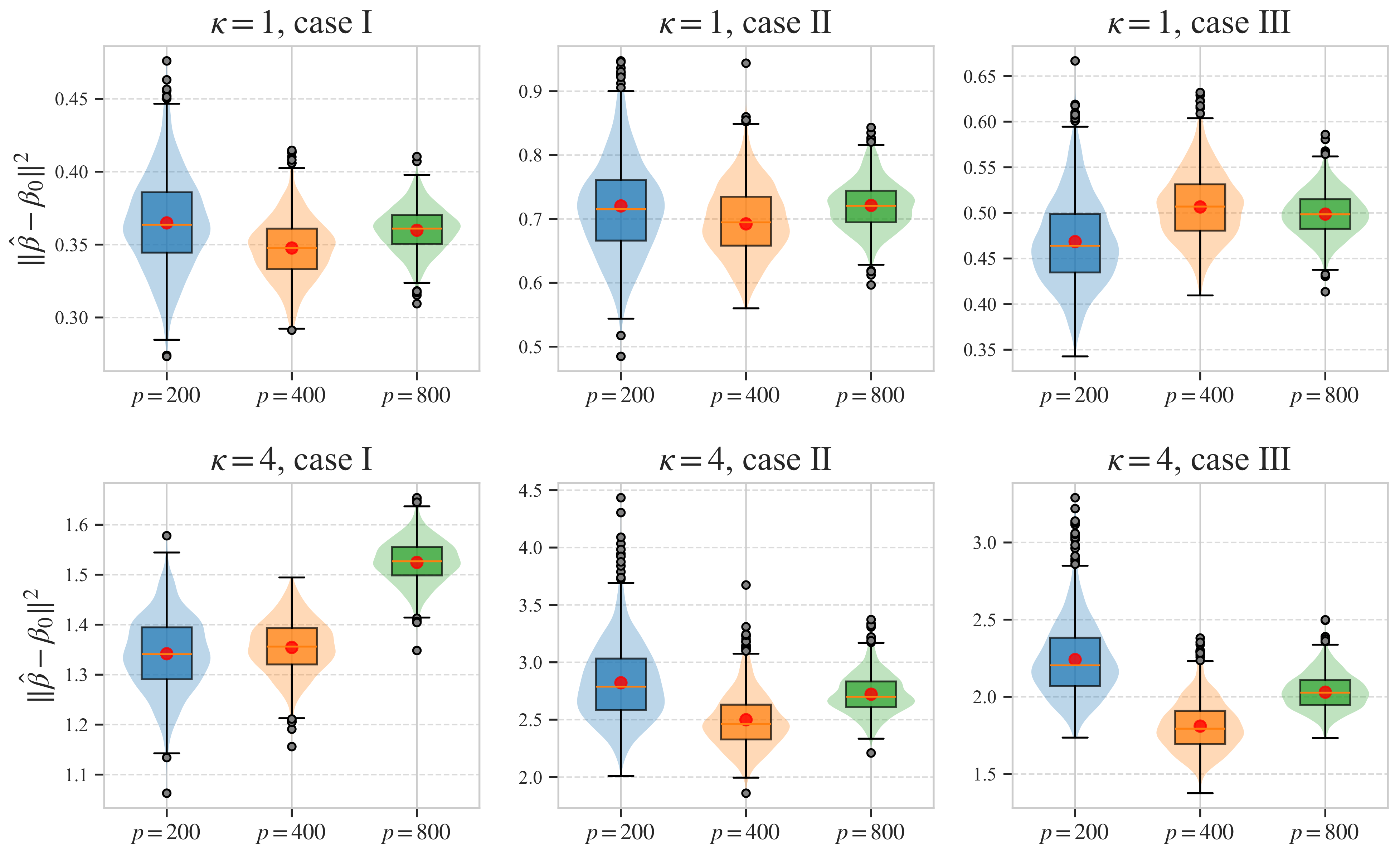
4.1. Validity of Theoretical Results

We first evaluate the validity of the proposed scalar $r_{\rho }$ in Theorem 1. For each setting, we generate ${\mathit{\beta }}^{\ast }$ and ${\mathit{w}}^{\ast }$ once with i.i.d. Unif$(0,1)$ entries and set ${\mathit{\beta }}_0={\mathit{\beta }}^{\ast }/\sqrt{n}$ and ${\mathit{w}}_0={\mathit{w}}^{\ast }/\sqrt{n}$. This construction yields diffuse coefficients whose Euclidean norms remain bounded as n grows. These coefficient vectors are fixed across the 1000 replications, while the target and source samples are regenerated in each replicate. In each replicate, we first compute $\widehat{\mathit{w}}$ from the source sample and then obtain $\widehat{\mathit{\beta }}$ by applying Algorithm 1, using the smoothed Huber loss (6) for both $\tilde{\rho }$ and $\rho$ with parameters $\delta =1.35$ and $\eta =0.1$. We fix $\tau ={\tau }_1=1$ and repeat each setup 1000 times.

Figure 1 presents boxplots of the estimation error $\parallel \widehat{\mathit{\beta }}-{\mathit{\beta }}_0{\parallel }^2$ for cases $\mathrm{I}$–$\mathrm{III}$ and $\kappa =1,4$. The red point in each boxplot marks the theoretical value $r_{\rho }^2$, obtained by numerically solving the system in Theorem 1 under the corresponding simulation specification. We observe that the empirical distribution of $\parallel \widehat{\mathit{\beta }}-{\mathit{\beta }}_0{\parallel }^2$ is centered close to this value, and its dispersion decreases as n and p become larger.

Table 1. Mean and SD (in parentheses) of $\parallel \widehat{\mathit{\beta }}-{\mathit{\beta }}_0{\parallel }^2$ (denoted as ${\widehat{r}}^2$) and the corresponding $r_{\rho }^2$ over 1000 simulations. Rows are indexed by $(p,n)$, with $n_1=2p$ when $\kappa =1$ and $n_1=p/2$ when $\kappa =4$.

($\mathit{p},\mathit{n}$)	Case $\mathbf{I}$		Case $\mathbf{II}$		Case $\mathbf{III}$
	${\widehat{\mathit{r}}}^{\mathbf{2}}$	${\mathit{r}}_{\mathit{\rho }}^{\mathbf{2}}$	${\widehat{\mathit{r}}}^{\mathbf{2}}$	${\mathit{r}}_{\mathit{\rho }}^{\mathbf{2}}$	${\widehat{\mathit{r}}}^{\mathbf{2}}$	${\mathit{r}}_{\mathit{\rho }}^{\mathbf{2}}$
$\kappa =1$
(200, 200)	0.3653 (0.0318)	0.3649	0.7163 (0.0738)	0.7204	0.4683 (0.0478)	0.4685
(400, 400)	0.3472 (0.0208)	0.3477	0.6970 (0.0549)	0.6923	0.5076 (0.0368)	0.5065
(800, 800)	0.3603 (0.0151)	0.3598	0.7206 (0.0374)	0.7212	0.4989 (0.0238)	0.4986
$\kappa =4$
(200, 50)	1.3415 (0.0734)	1.3419	2.8222 (0.3311)	2.8216	2.2410 (0.2407)	2.2415
(400, 100)	1.3565 (0.0531)	1.3544	2.4896 (0.2363)	2.4996	1.8087 (0.1590)	1.8102
(800, 200)	1.5261 (0.0427)	1.5247	2.7226 (0.1693)	2.7219	2.0342 (0.1153)	2.0301

shows the mean and standard deviation (SD) of $\parallel \widehat{\mathit{\beta }}-{\mathit{\beta }}_0{\parallel }^2$ (denoted as ${\widehat{r}}^2$) and the corresponding $r_{\rho }^2$ for each setup. As dimensionality increases, that is, as $\kappa$ increases from 1 to 4, both the mean error and its variability increase, indicating that estimation becomes more difficult in more challenging moderate–dimensional regimes. The average estimation error also grows with heavier-tailed errors, highlighting the difficulty of estimation under such conditions. Results under case $\mathrm{III}$ demonstrate that Theorem 1 is effective in handling non-identical ${\mathit{x}}_i$’s and ${ϵ}_i$’s. Overall, the findings in Figure 1 and Table 1 align well with the theoretical predictions of Theorem 1.

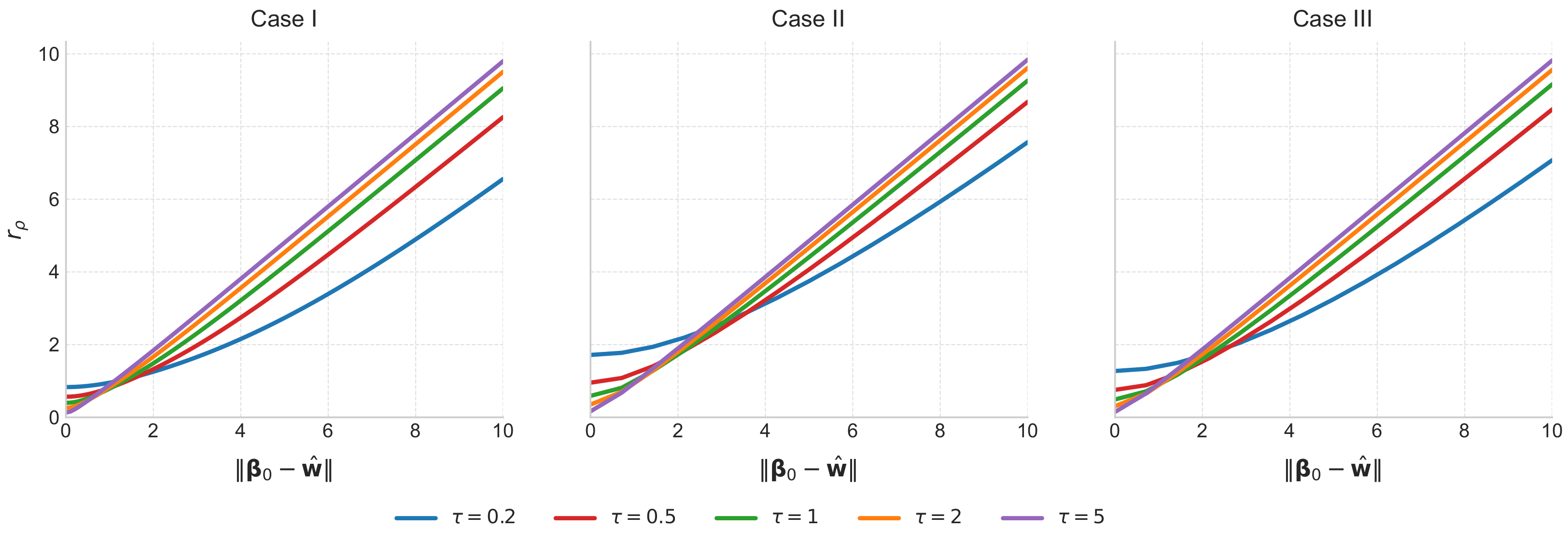
4.2. Theoretical Estimation Error Curves

We take $\rho$ to be our recommended smoothed Huber loss (6) with $(\delta ,\eta )=(1.35,0.1)$ and fix $\kappa =1$. We numerically solve the associated scalar system while varying the discrepancy term $\parallel {\mathit{\beta }}_0-\widehat{\mathit{w}}\parallel$ that enters the second equation of Theorem 1. Figure 2 plots the resulting curves of $r_{\rho }$ for five values of $\tau$ under cases $\mathrm{I}$–$\mathrm{III}$. In all three cases, the curves are monotonically increasing over the displayed range, so a larger $\parallel {\mathit{\beta }}_0-\widehat{\mathit{w}}\parallel$ corresponds to a larger asymptotic estimation error in this setting.

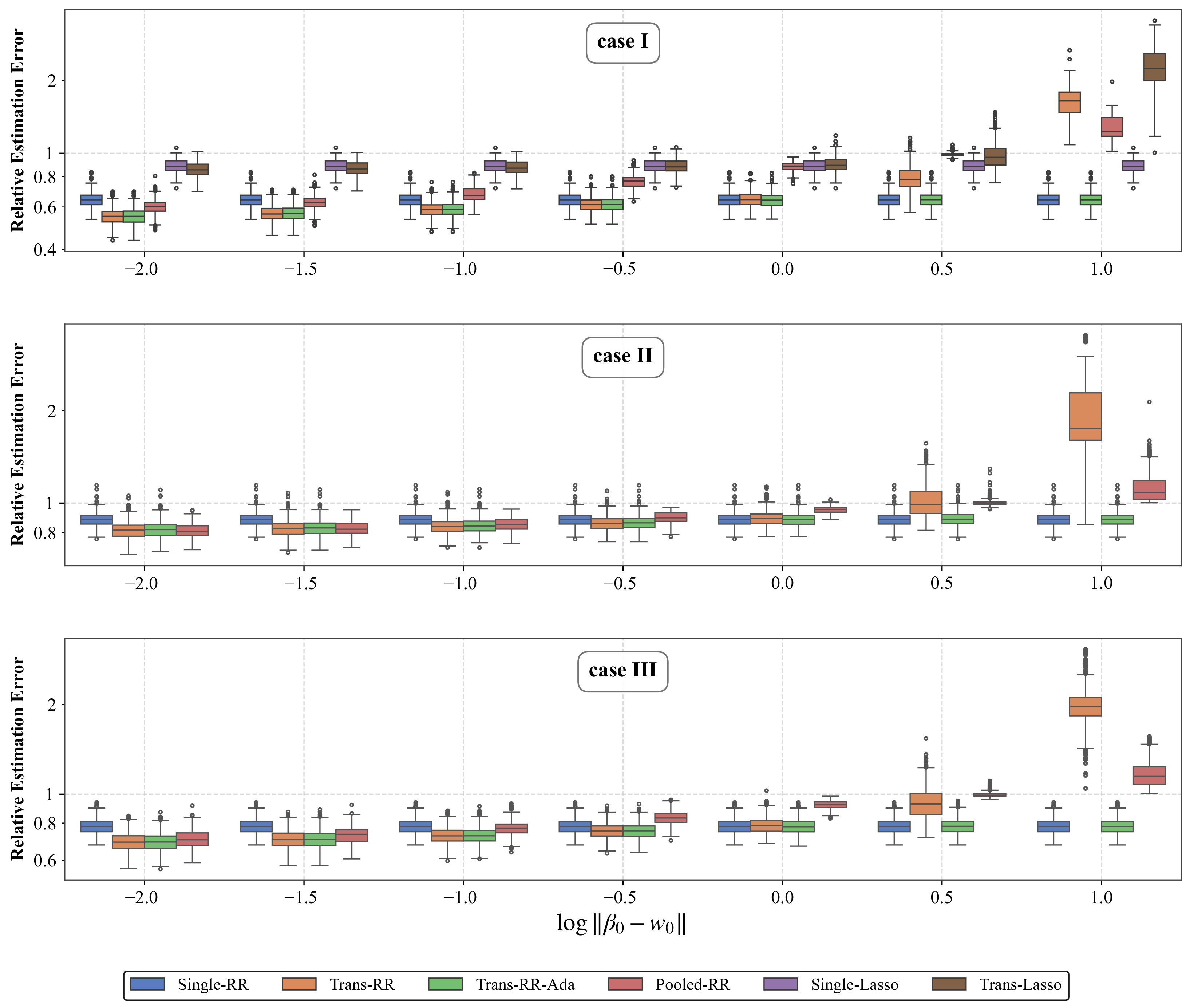
4.3. Comparison with Existing Methods

To evaluate when transfer is beneficial, we compare our method with several competing procedures across the three scenarios described above. We set $p=400$, $n=p$ and $n_1=2p$. We generate ${\mathit{\beta }}_0={\mathit{\beta }}^{\ast }/\parallel {\mathit{\beta }}^{\ast }\parallel$, where ${\mathit{\beta }}^{\ast }={({\mathit{\beta }}_1^{\ast },\dots ,{\mathit{\beta }}_p^{\ast })}^{\top }$ has i.i.d. Unif$(0,1)$ entries. To control the transfer strength $h=\parallel {\mathit{\delta }}_0\parallel$, we set

$${\mathit{\delta }}_0=\exp (c_d)·{\mathbf{1}}_p/\sqrt{p},c_d\in \{-2.0,-1.5,-1.0,-0.5,0,0.5,1.0\},$$

and define the source coefficient by ${\mathit{w}}_0={\mathit{\beta }}_0-{\mathit{\delta }}_0$. By varying $c_d$ from $-2.0$ to $1.0$, we obtain h ranging from approximately $0.135$ to $2.718$, providing a comprehensive evaluation across different levels of source-target similarity. For each value of $c_d$, the pair $({\mathit{\beta }}_0,{\mathit{w}}_0)$ is fixed across the 500 replications, and only the data are regenerated.

We compare four ridge-type methods (Single-RR, Trans-RR, Trans-RR-Ada, and Pooled-RR) and two lasso baselines (Single-Lasso and Trans-Lasso):

• Single-RR: The single-task estimator ${\widehat{\mathit{\beta }}}_{st}$ in (11), fit to the target sample alone.
• Trans-RR: The two-stage estimator $\widehat{\mathit{\beta }}=\widehat{\mathit{w}}+\widehat{\mathit{\delta }}$ in (5), computed by Algorithm 1.
• Trans-RR-Ada: The adaptive aggregate ${\widehat{\mathit{\beta }}}_{\mathrm{ada}}$ in (12), computed by Algorithm 2 with $K=5$, absolute-error loss $L(t)=\left|t\right|$, and weight grid $\mathrm{\Theta }=\{0,0.1,\dots ,0.9,1\}$.
• Pooled-RR: The same robust ridge fit applied to the concatenation of the source and target samples.
• Single-Lasso: The lasso on the target sample, with its regularization parameter chosen by $five$-fold cross-validation.
• Trans-Lasso: The two-stage transfer-lasso of [8], in which a cross-validated source-stage lasso estimates ${\mathit{w}}_0$ and a cross-validated target-stage lasso fits the residual $y_i-{\mathit{x}}_i^{\top }\widehat{\mathit{w}}$ on the target sample.

The four ridge-type methods all use the smoothed Huber loss (6) with $(\delta ,\eta )=(1.35,0.1)$. Each ridge penalty is tuned by $five$-fold cross-validation under the mean absolute error criterion, over the grid $\{3^a:a=-2,-3/2,\dots ,2\}$. For Trans-RR, the source penalty ${\tau }_1$ in (3) is tuned on the source sample, yielding $\widehat{\mathit{w}}$ as the minimizer of (3) at the tuned ${\tau }_1$. With $\widehat{\mathit{w}}$ held fixed, the target penalty $\tau$ in (4) is then tuned on the target sample.

Performance is summarized by the relative estimation error $\parallel \widehat{\mathit{\beta }}-{\mathit{\beta }}_0{\parallel }^2/{\parallel {\mathit{\beta }}_0\parallel }^2$. Figure 3 presents boxplots of these errors on a logarithmic scale, for varying values of h across cases $\mathrm{I}$–$\mathrm{III}$. We report all six estimators under Case $\mathrm{I}$. In Cases $\mathrm{II}$ and $\mathrm{III}$, the noise is heavy-tailed, and the lasso methods are not designed for robustness. Their fits failed to converge to stable estimates, so we restrict these two cases to the ridge-type methods.

Under Case $\mathrm{I}$, Trans-RR compares favorably with both lasso baselines, consistent with the non-sparse structure assumed throughout the paper. Among the ridge-type methods, Trans-RR outperforms Pooled-RR for small and moderate h across all three cases. Pooled-RR fits the source and target observations together as if they shared one coefficient, so its error reflects two mismatches: the gap between ${\mathit{\beta }}_0$ and ${\mathit{w}}_0$, and the difference between source and target noise levels. As h decreases, the gap between Pooled-RR and Trans-RR narrows, in line with the theoretical expectation that smaller h indicates greater similarity between the two domains.

More importantly, the comparison with Single-RR reveals the transition between positive and negative transfer. When h is small, Trans-RR achieves the lowest relative error among the ridge-type methods. As h grows, its advantage shrinks and eventually reverses. In our experiments, this turnover occurs near $h=1$. This is consistent with the numerical evidence in Section 3, since transfer is more favorable when the source-stage estimator is closer to the target coefficient. The same qualitative pattern appears in Cases $\mathrm{II}$ and $\mathrm{III}$, where the transition near $h=1$ persists under heavy-tailed errors and heterogeneous designs.

Trans-RR-Ada provides a data-driven safeguard against this negative transfer. Figure 3 shows that it tracks the better of Single-RR and Trans-RR for every value of h. For small h, Trans-RR-Ada essentially coincides with Trans-RR, while for large h it coincides with Single-RR. At the transition $h=1$, where Single-RR and Trans-RR are comparable, Trans-RR-Ada stays close to the better one.

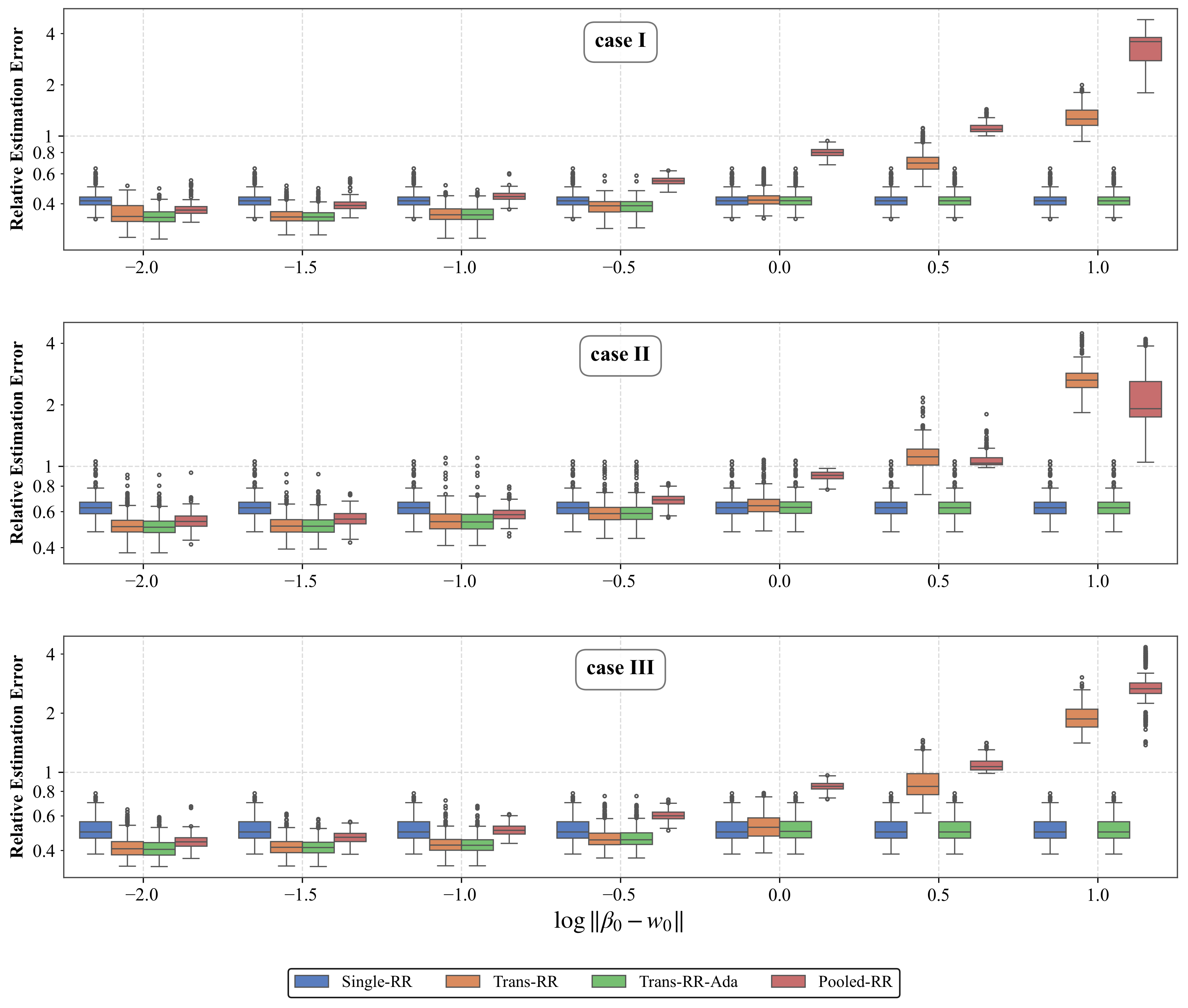
4.4. Robustness to Non-Identity Covariance

The asymptotic theory in Section 3 assumes $\mathrm{cov}({\mathit{x}}_i)={\mathit{I}}_p$. To verify that our methods remain effective under non-identity covariance, we re-run the comparison of Section 4.3 under AR(1) covariance ${\sum }_{jk}={\rho }^{|j-k|}$ with $\rho =0.6$, across all three noise cases $\mathrm{I}$, $\mathrm{II}$, and $\mathrm{III}$. All other settings, including the four ridge-type methods Single-RR, Trans-RR, Trans-RR-Ada, and Pooled-RR and the tuning protocol, match Section 4.3.

Figure 4 reports the resulting boxplots. The qualitative pattern of the i.i.d. comparison persists in all three cases. For small h, Trans-RR achieves the lowest error among the ridge-type methods. As h grows, its advantage shrinks and eventually reverses, with the transition again occurring near $h=1$. Trans-RR-Ada tracks the better of Single-RR and Trans-RR across all values of h. The negative-transfer transition and the safeguard role of Trans-RR-Ada are therefore not specific to the identity–covariance assumption underlying Theorem 1. This suggests that Trans-RR may remain effective under non-identity covariance.

4.5. Sensitivity to Tuning Choices

The comparison in Figure 3 fixes the smoothed Huber loss with $(\delta ,\eta )=(1.35,0.1)$ and selects each ridge penalty by $five$-fold cross-validation under the mean absolute error criterion, on a common geometric grid of nine values from $1/9$ to 9. This subsection examines whether the qualitative findings of that comparison are stable under perturbations to four tuning choices: the smoothed Huber parameters $(\delta ,\eta )$, the cross-validation criterion, the robust loss family, and the ridge penalty grid. Each perturbation re-runs the full simulation with $M=500$ replications per setting.

4.5.1. Choice of $(\delta ,\eta )$

The default $\delta =1.35$ is the standard Huber tuning. The smoothing parameter $\eta =0.1$ closely approximates the unsmoothed Huber loss and keeps ${\rho }_{\eta }$ twice continuously differentiable, as required by Assumption 1(b). In the sensitivity experiment, we vary $\delta$ over $\{1.0,1.35,2.0\}$ and $\eta$ over $\{0.05,0.10,0.20\}$, giving nine $(\delta ,\eta )$ pairs, and re-run the full simulation across the three cases and seven discrepancy values h for every pair. Within each $(\mathrm{case},h)$ combination, varying the $(\delta ,\eta )$ pair over the nine settings changes each method’s mean error by less than $7\%$ (median $1.5\%$) of its mean. The four-method ranking matches the default $(1.35,0.10)$ ranking in 171 of the 189 $(\mathrm{case},h,(\delta ,\eta ))$ cells. The qualitative findings are therefore stable under this perturbation.

Table 2. Sensitivity of relative estimation error to the smoothed Huber parameters $(\delta ,\eta )$ at the transition discrepancy $h=1$. Each entry reports Single-RR/Trans-RR/Trans-RR-Ada/Pooled-RR mean estimation error over $M=500$ replications. The three blocks correspond to the three error distributions of Section 4.3.

Case I (Gaussian Errors)
$\delta \setminus \eta$	$0.05$	$0.10$	$0.20$
$1.00$	0.653/0.655/0.651/0.883	0.654/0.656/0.652/0.883	0.656/0.658/0.654/0.883
$1.35$	0.644/0.647/0.642/0.882	0.645/0.647/0.642/0.882	0.646/0.648/0.643/0.882
$2.00$	0.641/0.642/0.637/0.885	0.640/0.642/0.637/0.885	0.641/0.643/0.637/0.885
Case II (Cauchy Errors)
$\delta \setminus \eta$	$0.05$	$0.10$	$0.20$
$1.00$	0.884/0.893/0.884/0.952	0.884/0.892/0.884/0.952	0.884/0.893/0.884/0.952
$1.35$	0.883/0.893/0.884/0.951	0.883/0.892/0.883/0.951	0.883/0.892/0.884/0.951
$2.00$	0.890/0.899/0.891/0.951	0.889/0.899/0.890/0.951	0.889/0.899/0.890/0.951
Case III (Mixture Errors)
$\delta \setminus \eta$	$0.05$	$0.10$	$0.20$
$1.00$	0.779/0.786/0.779/0.921	0.780/0.787/0.779/0.921	0.780/0.787/0.779/0.921
$1.35$	0.781/0.788/0.781/0.920	0.781/0.787/0.780/0.920	0.781/0.787/0.780/0.921
$2.00$	0.794/0.801/0.793/0.924	0.793/0.800/0.792/0.924	0.792/0.800/0.791/0.923

displays the four method means as a $(\delta ,\eta )$ heatmap at $h=1$ in each of the three cases. Within each $3\times 3$ grid, the entries vary only slightly and the four-method ordering is the same in every cell, illustrating the two findings stated above. Appendix B reports the heatmaps at the other six values of h, where the same pattern holds.

4.5.2. Choice of Cross-Validation Criterion

The default selects each ridge penalty by $five$-fold cross-validation under the mean absolute error criterion. We re-run the simulation with every cross-validation loss changed to mean squared error, keeping the smoothed Huber loss for estimation.

Table 3. Sensitivity of relative estimation error to the cross-validation criterion. All settings are as in Figure 3, except that every cross-validation loss (used to select ${\tau }_1$, $\tau$, ${\tau }_{\mathrm{st}}$, ${\tau }_{\mathrm{p}}$, and $\theta$) is changed from MAE to MSE. Each entry reports the default (MAE-CV) and the MSE-CV mean estimation error, in the format “default/MSE-CV”, over $M=500$ replications.

Case	h	Single-RR	Trans-RR	Trans-RR-Ada	Pooled-RR
$\mathrm{I}$	$0.135$	0.645/0.644	0.550/0.546	0.550/0.546	0.600/0.601
	$0.223$	0.645/0.644	0.565/0.561	0.566/0.561	0.628/0.629
	$0.368$	0.645/0.644	0.588/0.585	0.589/0.585	0.678/0.681
	$0.607$	0.645/0.644	0.616/0.614	0.617/0.615	0.764/0.770
	$1.000$	0.645/0.644	0.647/0.645	0.642/0.641	0.882/0.888
	$1.649$	0.645/0.644	0.791/0.793	0.645/0.644	0.990/0.991
	$2.718$	0.645/0.644	1.639/1.646	0.645/0.644	1.261/1.479
$\mathrm{II}$	$0.135$	0.883/1.772	0.816/2.582	0.819/1.895	0.811/1.324
	$0.223$	0.883/1.772	0.826/2.597	0.829/1.904	0.829/1.326
	$0.368$	0.883/1.772	0.840/2.618	0.843/1.915	0.855/1.353
	$0.607$	0.883/1.772	0.860/2.640	0.862/1.920	0.898/1.401
	$1.000$	0.883/1.772	0.892/2.745	0.883/1.963	0.951/1.497
	$1.649$	0.883/1.772	1.021/2.994	0.887/2.020	1.005/1.679
	$2.718$	0.883/1.772	1.898/3.827	0.883/2.108	1.123/2.223
$\mathrm{III}$	$0.135$	0.781/1.108	0.693/1.319	0.692/1.094	0.706/0.944
	$0.223$	0.781/1.108	0.707/1.334	0.707/1.102	0.729/0.966
	$0.368$	0.781/1.108	0.727/1.358	0.727/1.114	0.770/0.993
	$0.607$	0.781/1.108	0.754/1.395	0.754/1.138	0.834/1.054
	$1.000$	0.781/1.108	0.787/1.473	0.780/1.161	0.920/1.155
	$1.649$	0.781/1.108	0.941/1.749	0.783/1.194	0.998/1.368
	$2.718$	0.781/1.108	1.985/2.646	0.781/1.274	1.181/1.961

compares the mean estimation errors under the two criteria across all cases and values of h.

Under Case $\mathrm{I}$, the two criteria yield nearly identical mean errors and the same four-method ranking at every h. Under Cases $\mathrm{II}$ and $\mathrm{III}$, the mean errors of all four methods become substantially larger, and two qualitative findings of Section 4.3 no longer hold. First, Trans-RR has a larger mean error than Single-RR at every h in both heavy-tailed cases, so the range on which transfer helps disappears entirely. Second, Trans-RR-Ada no longer approximates min(Single-RR, Trans-RR) in most settings of the heavy-tailed cases. This may result from the heavy tails of Cauchy errors, under which MSE-based cross-validation is more sensitive to extreme residuals than MAE-based cross-validation. MAE-CV is therefore the appropriate default for heavy-tailed errors, and the conclusions of Section 4.3 are specific to this choice.

4.5.3. Choice of Robust Loss

In order to assess the sensitivity to the specific form of the robust loss, we replace the smoothed Huber loss in (6) with the pseudo-Huber loss ${\rho }_P(t;\delta )={\delta }^2\left(\sqrt{1+{(t/\delta )}^2}-1\right)$ at the same $\delta =1.35$.

Table 4. Sensitivity of relative estimation error to the choice of robust loss. All settings are as in Figure 3, except that the smoothed Huber loss is replaced by the pseudo-Huber loss ${\rho }_P(t;\delta )={\delta }^2(\sqrt{1+{(t/\delta )}^2}-1)$ with $\delta =1.35$ (the smoothing parameter $\eta$ is no longer needed). Each entry reports the default (smoothed Huber) and the pseudo-Huber mean estimation error, in the format “default/pseudo-Huber”, over $M=500$ replications.

Case	h	Single-RR	Trans-RR	Trans-RR-Ada	Pooled-RR
$\mathrm{I}$	$0.135$	0.645/0.645	0.550/0.545	0.550/0.546	0.600/0.595
	$0.223$	0.645/0.645	0.565/0.561	0.566/0.562	0.628/0.625
	$0.368$	0.645/0.645	0.588/0.585	0.589/0.586	0.678/0.675
	$0.607$	0.645/0.645	0.616/0.615	0.617/0.616	0.764/0.763
	$1.000$	0.645/0.645	0.647/0.647	0.642/0.643	0.882/0.883
	$1.649$	0.645/0.645	0.791/0.797	0.645/0.645	0.990/0.995
	$2.718$	0.645/0.645	1.639/1.642	0.645/0.645	1.261/1.299
$\mathrm{II}$	$0.135$	0.883/0.891	0.816/0.828	0.819/0.830	0.811/0.823
	$0.223$	0.883/0.891	0.826/0.836	0.829/0.839	0.829/0.839
	$0.368$	0.883/0.891	0.840/0.850	0.843/0.852	0.855/0.865
	$0.607$	0.883/0.891	0.860/0.869	0.862/0.872	0.898/0.905
	$1.000$	0.883/0.891	0.892/0.900	0.883/0.891	0.951/0.954
	$1.649$	0.883/0.891	1.021/1.023	0.887/0.895	1.005/1.007
	$2.718$	0.883/0.891	1.898/1.871	0.883/0.891	1.123/1.129
$\mathrm{III}$	$0.135$	0.781/0.793	0.693/0.703	0.692/0.703	0.706/0.713
	$0.223$	0.781/0.793	0.707/0.717	0.707/0.718	0.729/0.738
	$0.368$	0.781/0.793	0.727/0.740	0.727/0.740	0.770/0.777
	$0.607$	0.781/0.793	0.754/0.765	0.754/0.765	0.834/0.842
	$1.000$	0.781/0.793	0.787/0.798	0.780/0.791	0.920/0.925
	$1.649$	0.781/0.793	0.941/0.950	0.783/0.794	0.998/1.002
	$2.718$	0.781/0.793	1.985/1.972	0.781/0.793	1.181/1.199

compares the mean estimation errors under the two losses across all cases and values of h.

The mean errors are nearly identical to those under the smoothed Huber loss across all 21 settings. The four-method ranking matches the default in nearly every setting, and the few mismatches involve methods whose mean errors are essentially tied. The negative-transfer transition stays at the same value of h in every case, and Trans-RR-Ada continues to track min(Single-RR, Trans-RR) as closely as under the default. The qualitative findings of Section 4.3 are insensitive to this choice, consistent with Theorem 1.

4.5.4. Choice of Ridge Penalty Grid

The four ridge penalties ${\tau }_1$, $\tau$, ${\tau }_{\mathrm{st}}$, and ${\tau }_{\mathrm{p}}$ are tuned by $five$-fold cross-validation over a common geometric grid of nine values from $1/9$ to 9. We probe the sensitivity to this grid in two complementary ways: extending the grid to wider values, and forcing all four penalties to a common fixed value with no cross-validation.

We first extend the grid to thirteen values from $1/27$ to 27 on the same geometric scale, which contains the default grid as a strict subset.

Table 5. Sensitivity of relative estimation error to the ridge-penalty cross-validation grid. The default grid contains 9 values from $1/9$ to 9 on a geometric scale. The wide grid extends this to 13 values from $1/27$ to 27 on the same geometric scale, and contains the default grid as a strict subset. All other settings are as in Figure 3, with $M=500$ replications per cell. Each entry reports Single-RR/Trans-RR/Trans-RR-Ada/Pooled-RR mean estimation error.

Case	h	Default Grid (9 pts, [1/9, 9])	Wide Grid (13 pts, [1/27, 27])
$\mathrm{I}$	$0.135$	0.645/0.550/0.550/0.600	0.645/0.550/0.550/0.600
$\mathrm{I}$	$0.223$	0.645/0.565/0.566/0.628	0.645/0.565/0.566/0.628
$\mathrm{I}$	$0.368$	0.645/0.588/0.589/0.678	0.645/0.589/0.590/0.678
$\mathrm{I}$	$0.607$	0.645/0.616/0.617/0.764	0.645/0.618/0.619/0.764
$\mathrm{I}$	$1.000$	0.645/0.647/0.642/0.882	0.645/0.648/0.642/0.883
$\mathrm{I}$	$1.649$	0.645/0.791/0.645/0.990	0.645/0.791/0.645/0.990
$\mathrm{I}$	$2.718$	0.645/1.639/0.645/1.261	0.645/1.639/0.645/1.261
$\mathrm{II}$	$0.135$	0.883/0.816/0.819/0.811	0.887/0.824/0.826/0.811
$\mathrm{II}$	$0.223$	0.883/0.826/0.829/0.829	0.887/0.835/0.838/0.829
$\mathrm{II}$	$0.368$	0.883/0.840/0.843/0.855	0.887/0.850/0.852/0.856
$\mathrm{II}$	$0.607$	0.883/0.860/0.862/0.898	0.887/0.869/0.871/0.900
$\mathrm{II}$	$1.000$	0.883/0.892/0.883/0.951	0.887/0.896/0.888/0.955
$\mathrm{II}$	$1.649$	0.883/1.021/0.887/1.005	0.887/1.021/0.891/1.006
$\mathrm{II}$	$2.718$	0.883/1.898/0.883/1.123	0.887/1.899/0.887/1.120
$\mathrm{III}$	$0.135$	0.781/0.693/0.692/0.706	0.782/0.694/0.694/0.706
$\mathrm{III}$	$0.223$	0.781/0.707/0.707/0.729	0.782/0.709/0.709/0.729
$\mathrm{III}$	$0.368$	0.781/0.727/0.727/0.770	0.782/0.731/0.731/0.770
$\mathrm{III}$	$0.607$	0.781/0.754/0.754/0.834	0.782/0.758/0.758/0.834
$\mathrm{III}$	$1.000$	0.781/0.787/0.780/0.920	0.782/0.789/0.781/0.922
$\mathrm{III}$	$1.649$	0.781/0.941/0.783/0.998	0.782/0.941/0.783/0.999
$\mathrm{III}$	$2.718$	0.781/1.985/0.781/1.181	0.782/1.985/0.782/1.180

compares the mean estimation errors under the default and the wide grid across all cases and values of h. The impact on estimation is negligible: each method’s mean error barely changes across settings, the four-method ranking is unchanged except at settings with near-tied means, the negative-transfer transition does not move, and Trans-RR-Ada continues to track min(Single-RR, Trans-RR) as closely as under the default. The default grid is therefore wide enough on both sides, and the qualitative findings of Section 4.3 do not depend on the choice of upper or lower endpoint.

We next force all four ridge penalties to a common fixed value $\tau \in \{1/3,1,3,9\}$, removing the ridge cross-validation entirely. Trans-RR-Ada’s mixing weight $\theta$ is still selected by $five$-fold cross-validation on the target sample (Algorithm 2).

Table 6. Sensitivity of relative estimation error to the ridge penalty value when cross-validation tuning is disabled. All four ridge penalties (Single-RR’s ${\tau }_{\mathrm{st}}$, Trans-RR’s ${\tau }_1$ and $\tau$, Pooled-RR’s ${\tau }_{\mathrm{p}}$) are forced to a common fixed value from $\{1/3,1,3,9\}$. Trans-RR-Ada’s mixing weight $\theta$ is still selected by 5-fold cross-validation on the target sample (Algorithm 2). All other settings are as in Figure 3, with $M=500$ replications per cell. Each entry reports Single-RR/Trans-RR/Trans-RR-Ada/Pooled-RR mean estimation error.

Case	h	τ = 1/3	τ = 1	τ = 3	τ = 9
$\mathrm{I}$	$0.135$	0.742/0.769/0.687/0.619	0.628/0.523/0.525/0.605	0.742/0.620/0.620/0.773	0.881/0.814/0.814/0.906
$\mathrm{I}$	$0.223$	0.742/0.781/0.696/0.645	0.628/0.538/0.538/0.625	0.742/0.631/0.632/0.783	0.881/0.820/0.820/0.910
$\mathrm{I}$	$0.368$	0.742/0.804/0.709/0.694	0.628/0.565/0.561/0.661	0.742/0.651/0.652/0.801	0.881/0.829/0.829/0.917
$\mathrm{I}$	$0.607$	0.742/0.851/0.728/0.790	0.628/0.616/0.596/0.726	0.742/0.687/0.690/0.833	0.881/0.846/0.846/0.929
$\mathrm{I}$	$1.000$	0.742/0.953/0.745/0.990	0.628/0.714/0.629/0.848	0.742/0.752/0.740/0.890	0.881/0.876/0.876/0.951
$\mathrm{I}$	$1.649$	0.742/1.185/0.743/1.423	0.628/0.913/0.628/1.074	0.742/0.866/0.742/0.986	0.881/0.924/0.881/0.986
$\mathrm{I}$	$2.718$	0.742/1.739/0.742/2.321	0.628/1.287/0.628/1.436	0.742/1.033/0.742/1.113	0.881/0.987/0.881/1.030
$\mathrm{II}$	$0.135$	2.026/2.443/2.014/1.143	0.978/0.964/0.930/0.789	0.861/0.778/0.784/0.850	0.924/0.877/0.878/0.936
$\mathrm{II}$	$0.223$	2.026/2.459/2.019/1.167	0.978/0.979/0.938/0.804	0.861/0.787/0.793/0.857	0.924/0.881/0.882/0.939
$\mathrm{II}$	$0.368$	2.026/2.490/2.027/1.211	0.978/1.005/0.953/0.833	0.861/0.803/0.810/0.870	0.924/0.888/0.889/0.943
$\mathrm{II}$	$0.607$	2.026/2.551/2.037/1.297	0.978/1.055/0.972/0.885	0.861/0.832/0.836/0.894	0.924/0.900/0.903/0.952
$\mathrm{II}$	$1.000$	2.026/2.681/2.045/1.475	0.978/1.152/0.988/0.983	0.861/0.885/0.865/0.937	0.924/0.923/0.922/0.968
$\mathrm{II}$	$1.649$	2.026/2.971/2.042/1.848	0.978/1.342/0.984/1.161	0.861/0.977/0.864/1.008	0.924/0.959/0.927/0.994
$\mathrm{II}$	$2.718$	2.026/3.615/2.034/2.569	0.978/1.663/0.978/1.420	0.861/1.096/0.861/1.093	0.924/1.000/0.925/1.022
$\mathrm{III}$	$0.135$	1.286/1.442/1.246/0.827	0.784/0.713/0.704/0.686	0.798/0.693/0.694/0.808	0.902/0.844/0.844/0.920
$\mathrm{III}$	$0.223$	1.286/1.456/1.253/0.852	0.784/0.729/0.715/0.705	0.798/0.703/0.704/0.817	0.902/0.849/0.849/0.923
$\mathrm{III}$	$0.368$	1.286/1.484/1.265/0.900	0.784/0.756/0.735/0.737	0.798/0.721/0.724/0.833	0.902/0.857/0.857/0.929
$\mathrm{III}$	$0.607$	1.286/1.541/1.282/0.994	0.784/0.808/0.763/0.797	0.798/0.754/0.759/0.861	0.902/0.872/0.873/0.940
$\mathrm{III}$	$1.000$	1.286/1.661/1.294/1.187	0.784/0.909/0.789/0.910	0.798/0.815/0.799/0.912	0.902/0.898/0.899/0.959
$\mathrm{III}$	$1.649$	1.286/1.933/1.290/1.600	0.784/1.109/0.786/1.115	0.798/0.920/0.799/0.996	0.902/0.941/0.903/0.990
$\mathrm{III}$	$2.718$	1.286/2.559/1.286/2.420	0.784/1.466/0.784/1.426	0.798/1.064/0.798/1.103	0.902/0.993/0.902/1.026

reports the mean estimation errors at the four fixed $\tau$ values across all cases and values of h. At every fixed $\tau$, the mean error of Trans-RR grows monotonically with h in all three cases, consistent with the theoretical risk curves of Figure 2. The absolute levels and the four-method ranking do vary substantially across the four $\tau$ values, but the qualitative dependence on h predicted by the theory is preserved at every $\tau$.

The Trans-RR-Ada safeguard nevertheless remains effective: its mean error stays close to min(Single-RR, Trans-RR) in every one of the 84 settings, just as under cross-validated penalties. The agreement between Trans-RR-Ada and min(Single-RR, Trans-RR) is therefore robust to a misspecified ridge penalty.

5. Real Data Analysis

We evaluate the proposed transfer procedure on the near-infrared (NIR) spectral dataset from the 2002 International Diffuse Reflectance Conference (IDRC) “Shootout” competition. The data consist of pharmaceutical tablet measurements collected by two spectrometers, with ASSAY as the response. For each instrument, the dataset contains a training sample of size 460 and an external test sample of size 155. Each spectrum is recorded at 650 wavelengths, yielding a moderate–dimensional regression problem.

Let X and $X_1$ denote the spectra from the two instruments. We consider two transfer directions. In Direction A, X is the target domain and $X_1$ is the source domain. In Direction B, the roles are reversed. In each repetition, we randomly split the training sample of the target instrument into two parts of sizes 160 and 300. The subset of size 160 is used as the target training sample. The remaining 300 tablets are matched with their measurements from the other instrument to form the source training sample. When X is the target domain, the target fit is constructed from 160 observations in X, and the source fit is constructed from the corresponding 300 observations in $X_1$. The same scheme is applied symmetrically in the reverse direction. The external test sample of the target instrument is used for evaluation. We repeat this procedure 20 times to reduce Monte Carlo variability.

The preprocessing used in both transfer directions has two stages. First, we thin the spectrum by retaining every fourth wavelength of the original 650, yielding $p=163$ predictors. Two considerations motivate this thinning. Adjacent NIR wavelengths record highly overlapping absorption signals, so a four-fold thinning preserves nearly all the spectral information. This is standard practice in NIR chemometrics. A step of four also gives $p=163\approx n=160$, the same $p/n\approx 1$ setting as in our simulations.

Second, for each domain, predictors are whitened using its own training sample,

$$\tilde{X}=(X-\widehat{\mu }){\displaystyle {\widehat{\sum }}^{-1/2}},$$

where $\widehat{\mu }$ and ${\displaystyle \widehat{\sum }}$ are estimated from that training sample, and the same transformation is applied to the associated test sample. Whitening decorrelates the highly collinear NIR predictors so that the sample second-moment matrix of $\tilde{X}$ approximates ${\mathit{I}}_p$, which is the design assumption underlying Theorem 1. The response is centered using the mean of the corresponding training response, and the same centering constant is used for the associated test response. All preprocessing parameters are thus estimated only on training data and carried over to the test set, avoiding information leakage.

We compare six methods: Single-RR, Trans-RR, the adaptive Trans-RR estimator ${\widehat{\mathit{\beta }}}_{\mathrm{ada}}$ from Section 3.3 (denoted Trans-RR-Ada in the table), Pooled-RR, Single-Lasso, and Trans-Lasso. For the ridge-type methods, we use the smoothed Huber loss in (6) with $(\delta ,\eta )=(1.35,0.1)$. All tuning parameters are selected by 5-fold cross-validation with mean absolute error as the validation criterion, from the common grid

$$\mathcal{G}=\{{10}^{-5},{10}^{-4.5},{10}^{-4},\dots ,{10}^1\}.$$

Performance is measured by the test-set RMSE,

$$\mathrm{RMSE}=\sqrt{{\displaystyle \frac{1}{n_{\mathrm{test}}}}{\sum }_{i=1}^{n_{\mathrm{test}}}{(y_i-{\widehat{y}}_i)}^2},$$

where $y_i$ and ${\widehat{y}}_i$ are on the original ASSAY scale (predictions are uncentered before evaluation) and $n_{\mathrm{test}}=155$ in both transfer directions.

Table 7. Prediction performance on the NIR spectral dataset over 20 repeated random splits. Each entry reports the average RMSE, with the standard deviation in parentheses.

Method	Direction A	Direction B
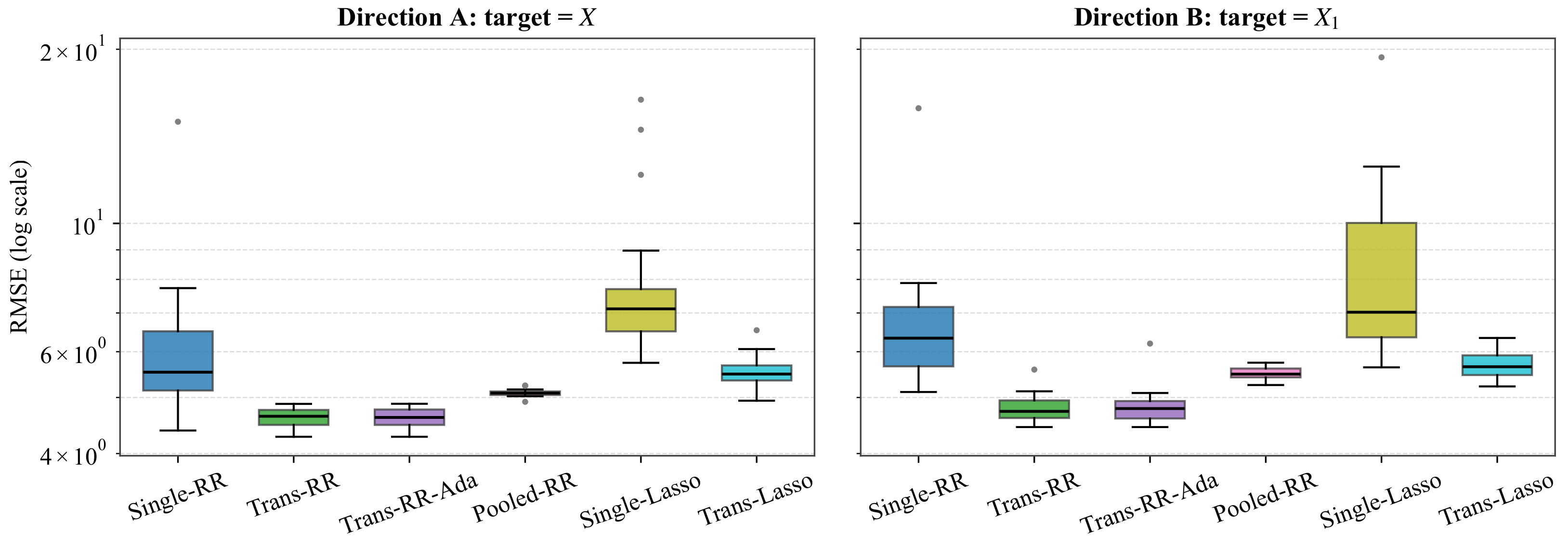
Trans-RR	4.6230 (0.1732)	4.7933 (0.2736)
Trans-RR-Ada	4.6294 (0.1861)	4.8211 (0.3757)
Pooled-RR	5.0952 (0.0812)	5.4909 (0.1335)
Trans-Lasso	5.5668 (0.3650)	5.6803 (0.3131)
Single-RR	6.2666 (2.2628)	6.8272 (2.2674)
Single-Lasso	8.0672 (2.8904)	8.5607 (3.3739)

reports the average RMSE and its standard deviation over the 20 repetitions, and Figure 5 displays the corresponding distributional information. Trans-RR achieves the smallest mean RMSE in both transfer directions, with relatively small variability across the 20 splits. The adaptive variant Trans-RR-Ada matches Trans-RR within $0.03$ in mean RMSE in both directions, indicating that the source and target are close enough for transfer to be uniformly beneficial on this dataset. Pooled-RR ranks third behind the two transfer-ridge methods and is uniformly dominated by Trans-RR, suggesting that naive pooling fails to account for cross-instrument differences. The lasso methods are less competitive overall, especially Single-Lasso. This is consistent with the non-sparse structure of NIR spectra, where relevant information is distributed over broad wavelength regions rather than concentrated on a small subset of predictors.

We further checked the procedure for four starting offsets of the every-fourth-wavelength thinning and for the same procedure without whitening. Across all five resulting preprocessing variants and both transfer directions, Trans-RR and Trans-RR-Ada are the top two methods by mean RMSE, and their mean RMSE values differ by at most $0.05$. Mean RMSE for all six methods in each variant and direction is reported in Appendix C. The results, together with these robustness checks, therefore support the effectiveness of the proposed Trans-RR method.

6. Discussion

This paper introduces Trans-RR, a robust transfer-learning approach for moderate–dimensional linear regression. It extends transfer-learning ideas of [7,8] to a setting with non-sparse coefficients and heavy-tailed errors, without relying on sparsity assumptions or moment restrictions on the errors. The theory and the numerical results show that negative transfer can occur when the source study is not sufficiently informative for the target study. To guard against this, we also propose an adaptive aggregation of Trans-RR with the single-task estimator that selects the mixing weight by cross-validation. The theoretical results, simulation studies, and real-data analysis support the effectiveness of both procedures. A natural direction for further study is to identify the choice of loss function that minimizes the asymptotic estimation error in our framework.

References

- Chen, M. Analysis on transfer learning models and applications in natural language processing. Highlights Sci. Eng. Technol. 2022, 16, 446–452. [Google Scholar] [CrossRef]
- Ma, Y.; Chen, S.; Ermon, S.; Lobell, D.B. Transfer learning in environmental remote sensing. Remote Sens. Environ. 2024, 301, 113924. [Google Scholar] [CrossRef]
- Gopalakrishnan, K.; Khaitan, S.K.; Choudhary, A.; Agrawal, A. Deep convolutional neural networks with transfer learning for computer vision-based data-driven pavement distress detection. Constr. Build. Mater. 2017, 157, 322–330. [Google Scholar] [CrossRef]
- Liu, D.; Luo, J.; Johnson, B.; Chew, H.; Blais, J.; Deik, A.; Paul, F.; Hanson, R.L.; Crandall, J.P.; Sun, Y.; et al. Modeling blood metabolite homeostatic levels reduces sample heterogeneity across cohorts. Proc. Natl. Acad. Sci. USA 2024, 121, e2307430121. [Google Scholar] [CrossRef]
- Chen, A.; Owen, A.B.; Shi, M. Data enriched linear regression. Electron. J. Stat. 2015, 9, 1078–1112. [Google Scholar] [CrossRef]
- Tripuraneni, N.; Jin, C.; Jordan, M. Provable meta-learning of linear representations. In Proceedings of the 38th International Conference on Machine Learning, Virtual, 18–24 July 2021; Volume 139, pp. 10434–10443. [Google Scholar]
- Bastani, H. Predicting with proxies: Transfer learning in high dimension. Manag. Sci. 2021, 67, 2964–2984. [Google Scholar] [CrossRef]
- Li, S.; Cai, T.T.; Li, H. Transfer learning for high-dimensional linear regression: Prediction, estimation and minimax optimality. J. R. Stat. Soc. Ser. B Stat. Methodol. 2022, 84, 149–173. [Google Scholar] [CrossRef]
- Tian, Y.; Feng, Y. Transfer learning under high-dimensional generalized linear models. J. Am. Stat. Assoc. 2023, 118, 2684–2697. [Google Scholar] [CrossRef]
- Li, S.; Zhang, L.; Cai, T.T.; Li, H. Estimation and inference for high-dimensional generalized linear models with knowledge transfer. J. Am. Stat. Assoc. 2024, 119, 1274–1285. [Google Scholar] [CrossRef]
- Cai, T.T.; Wei, H. Transfer learning for nonparametric classification: Minimax rate and adaptive classifier. Ann. Stat. 2021, 49, 100–128. [Google Scholar] [CrossRef]
- Cai, T.T.; Pu, H. Transfer learning for nonparametric regression: Non-asymptotic minimax analysis and adaptive procedure. arXiv 2024, arXiv:2401.12272. [Google Scholar] [CrossRef]
- Fan, J.; Gao, C.; Klusowski, J.M. Robust transfer learning with unreliable source data. arXiv 2023, arXiv:2310.04606. [Google Scholar] [CrossRef]
- Huber, P.J. Robust regression: Asymptotics, conjectures and Monte Carlo. Ann. Stat. 1973, 1, 799–821. [Google Scholar] [CrossRef]
- Portnoy, S. Asymptotic behavior of M-estimators of p regression parameters when p2/n is large. I. Consistency. Ann. Stat. 1984, 13, 1298–1309. [Google Scholar]
- Portnoy, S. Asymptotic behavior of M-estimators of p regression parameters when p2/n is large. II. Normal approximation. Ann. Stat. 1985, 13, 1403–1417. [Google Scholar] [CrossRef]
- Portnoy, S. Asymptotic behavior of the empiric distribution of M-estimated residuals from a regression model with many parameters. Ann. Stat. 1986, 14, 1152–1170. [Google Scholar] [CrossRef]
- Portnoy, S. A central limit theorem applicable to robust regression estimators. J. Multivar. Anal. 1987, 22, 24–50. [Google Scholar] [CrossRef][Green Version]
- Mammen, E. Asymptotics with increasing dimension for robust regression with applications to the bootstrap. Ann. Stat. 1989, 17, 382–400. [Google Scholar] [CrossRef]
- El Karoui, N.; Bean, D.; Bickel, P.J.; Lim, C.; Yu, B. On robust regression with high-dimensional predictors. Proc. Natl. Acad. Sci. USA 2013, 110, 14557–14562. [Google Scholar] [CrossRef]
- El Karoui, N. On the impact of predictor geometry on the performance on high-dimensional ridge-regularized generalized robust regression estimators. Probab. Theory Relat. Fields 2018, 170, 95–175. [Google Scholar] [CrossRef]
- Charbonnier, P.; Blanc-Feraud, L.; Aubert, G.; Barlaud, M. Deterministic edge-preserving regularization in computed imaging. IEEE Trans. Image Process. 1997, 6, 298–311. [Google Scholar] [CrossRef]
- Hartley, R.; Zisserman, A. Multiple View Geometry in Computer Vision; Cambridge University Press: Cambridge, UK, 2003. [Google Scholar]
- Yohai, V.J.; Maronna, R.A. Asymptotic behavior of M-estimators for the linear model. Ann. Stat. 1979, 7, 258–268. [Google Scholar] [CrossRef]
- El Karoui, N. Asymptotic behavior of unregularized and ridge-regularized high-dimensional robust regression estimators: Rigorous results. arXiv 2013, arXiv:1311.2445. [Google Scholar]
- El Karoui, N. Concentration of measure and spectra of random matrices: Applications to correlation matrices, elliptical distributions and beyond. Ann. Appl. Probab. 2009, 19, 2362–2405. [Google Scholar] [CrossRef]
- Ledoux, M. The Concentration of Measure Phenomenon; American Mathematical Society: Providence, RI, USA, 2001; Volume 89. [Google Scholar]
- Huber, P.J.; Ronchetti, E.M. Robust Statistics; John Wiley & Sons: Hoboken, NJ, USA, 2009. [Google Scholar]
- Karlin, S. Total Positivity; Stanford University Press: Stanford, CA, USA, 1968. [Google Scholar]
- Ibragimov, I.A. On the composition of unimodal distributions. Teor. Veroyatnost. Primen. 1956, 1, 283–288. [Google Scholar] [CrossRef]
- Dharmadhikari, S.; Joag-Dev, K. Unimodality, Convexity, and Applications; Probability and Mathematical Statistics; Academic Press, Inc.: Boston, MA, USA, 1988. [Google Scholar]
- Moreau, J.J. Proximité et dualité dans un espace hilbertien. Bull. Soc. Math. Fr. 1965, 93, 273–299. [Google Scholar] [CrossRef]
- Beck, A.; Teboulle, M. Gradient-based algorithms with applications to signal-recovery problems. In Convex Optimization in Signal Processing and Communications; Palomar, D.P., Eldar, Y.C., Eds.; Cambridge University Press: Cambridge, UK, 2010; pp. 42–88. [Google Scholar]
- Bean, D.; Bickel, P.J.; El Karoui, N.; Yu, B. Optimal M-estimation in high-dimensional regression. Proc. Natl. Acad. Sci. USA 2013, 110, 14563–14568. [Google Scholar] [CrossRef]
- Efron, B.; Stein, C. The jackknife estimate of variance. Ann. Stat. 1981, 9, 586–596. [Google Scholar] [CrossRef]
- Bhatia, R. Matrix Analysis; Springer: New York, NY, USA, 1997. [Google Scholar]
- Johnson, C.R.; Horn, R.A. Matrix Analysis; Cambridge University Press: Cambridge, UK, 1985. [Google Scholar]
- Stroock, D.W. Probability Theory: An Analytic View; Cambridge University Press: Cambridge, UK, 2010. [Google Scholar]
- van der Vaart, A.W. Asymptotic Statistics; Cambridge University Press: Cambridge, UK, 2000. [Google Scholar]