High-Quality Representation Learning Approach to Spatio-Temporal Traffic Speed Data with Lp,ϵ-Norm


Abstract
1. Introduction
- 1.
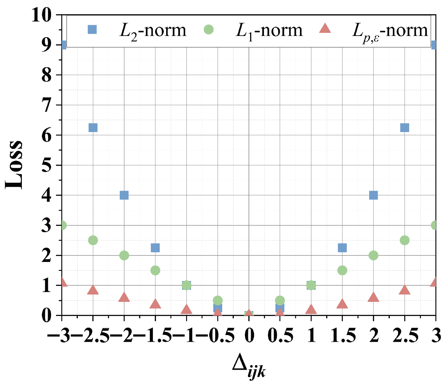
- It constructs a learning objective grounded in the Lp,ϵ-norm. As a result, it achieves accurate reconstruction of missing values from partially observed traffic data.
- 2.
- The model’s parameters are automatically adjusted using a fuzzy controller for high scalability.
2. Related Work
3. Preliminaries
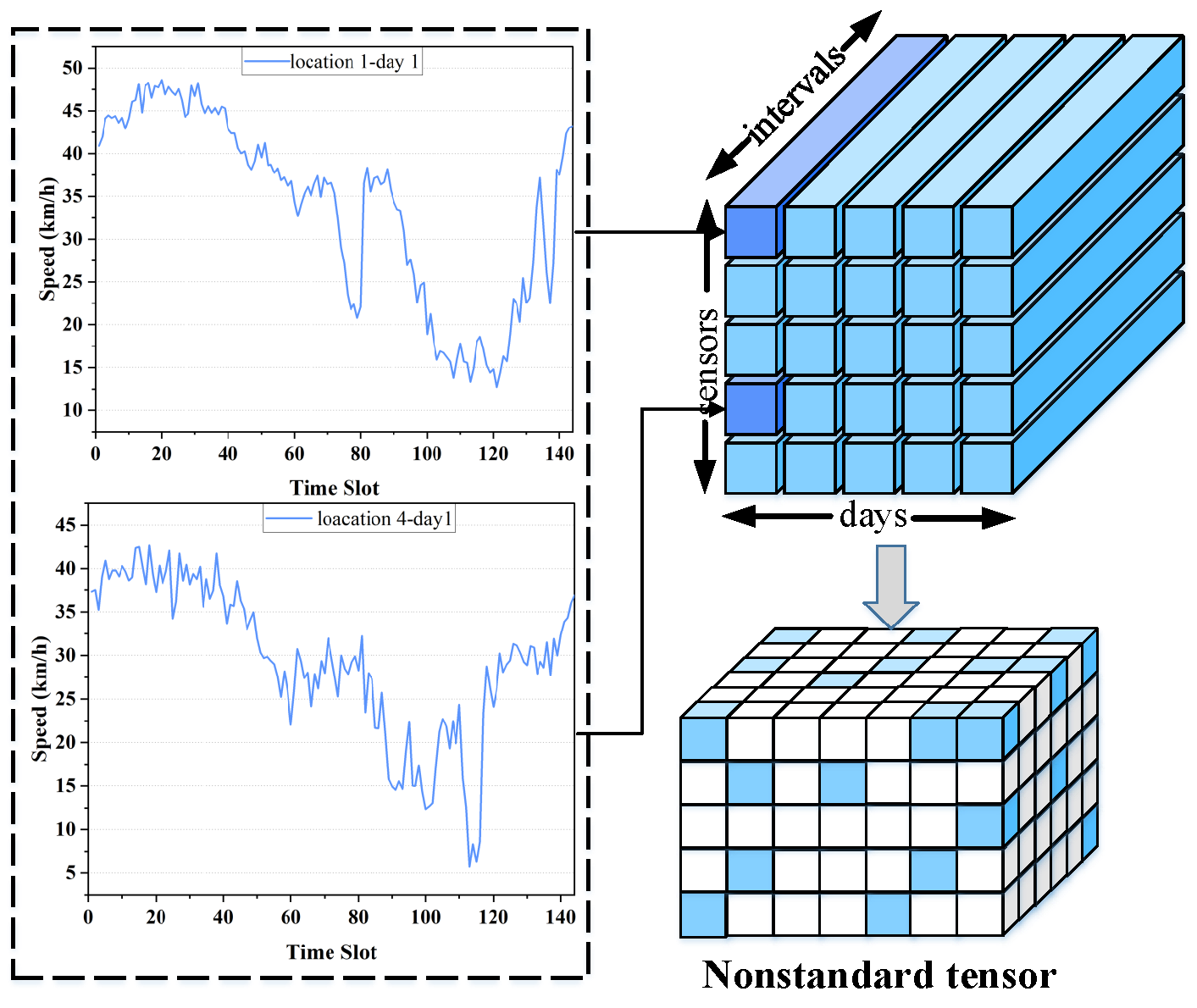
3.1. Data Recovery Problem in ITS
3.2. Latent Factorization of Tensors (LFT)
3.3. Fuzzy Control
4. Proposed Lp,ϵLFT Model
4.1. Generalized Objective Function
4.2. SGD-Based Learning Rules
4.3. Fuzzy Reasoning Rule Designing
- 1.
- As training progresses, the model error gradually decreases and the parameters progressively approach their optimal value. At this stage, it becomes crucial to reduce the step size to mitigate oscillations around the optimal solution, thereby enhancing the stability of the optimization process. To prevent premature convergence to a local optimum and the consequent model instability, it is advisable to progressively decrease the step size as the model error diminishes throughout the training process.
- 2.
- As model training progresses and the error diminishes, gradually increasing the regularization coefficient is effective in alleviating overfitting and enhancing the model’s generalization capacity. During the initial training phases, when the error remains relatively high, a smaller allows more flexible model parameter adjustments, thereby accelerating error reduction. Conversely, in the later stages of training, as the error declines, increasing effectively regulates model complexity, thereby preventing overfitting to noise within the training data and enhancing performance and robustness on unseen datasets.
- 3.
- In the early stages of training, when the model error remains relatively high and the influence of outliers on the overall trend is limited, maintaining a relatively large p enables the model to adapt with greater flexibility. This facilitates rapid identification of the underlying data patterns without excessively suppressing informative signals. As training progresses and the model error decreases, the relative impact of outliers becomes more pronounced. If p remains large, the model may be negatively affected by outliers, leading to fluctuations and instability in the vicinity of the optimal solution. Therefore, in the later stages of training, a gradual reduction of p plays a crucial role in suppressing the influence of outliers, thereby enhancing the robustness and stability of the model and mitigating the risk of noise driving the parameters away from the optimal solution.
- 4.
- In the early stages of training, when the model error remains relatively high and achieving rapid yet stable progress is a priority, maintaining a relatively large is beneficial. A large enhances the smoothness and convexity of the Lp,ϵ-norm, leading to stable gradient behavior and facilitating efficient optimization without being trapped by sharp or ill-conditioned penalty geometries. As training progresses and the model error decreases, fidelity to the true p-norm becomes increasingly important for suppressing the influence of outliers. Therefore, in the latter stages of training, it is advisable to gradually reduce , thereby ensuring that the penalty more closely approximates the original p-norm and enforces stronger robustness. This strategy balances the final model’s expressivity and robustness against numerical stability by starting with larger smoothing to accelerate and stabilize convergence and ending with smaller smoothing to recover the desired p-norm behavior.
4.4. Algorithm Design and Analysis
| Algorithm 1 Lp,ϵLFT |
Operation Cost |
5. Experimental Results and Analysis
5.1. General Settings
- Datasets: An empirical study was conducted using publicly available traffic speed datasets from six major urban areas, namely Guangzhou (China), Seattle, New York, Los Angeles, San Francisco (USA), and Berlin (Germany). The corresponding descriptions of these datasets are presented below.
- D1: Guangzhou Traffic Speed Dataset [33]. These dataset contains measurements collected from 214 monitoring devices in Guangzhou, China, recorded at 10 min intervals over a 61-day period (1 August–30 September 2016).
- D2: Seattle Dataset, obtained from the Uber movement project (https://github.com/xinychen/tracebase?tab=readme-ov-file, accessed on 7 January 2026), contains traffic speed data collected from 20,833 detectors in Seattle, WA, USA, recorded hourly over the period 1–31 January 2020.
- D3: New York Speed Dataset, (https://www.kaggle.com/datasets/crailtap/nyc-real-time-traffic-speed-data-feed, accessed on 7 January 2026 ) includes data collected from 135 monitoring devices in New York, USA, over a 73 days period (1 October–12 December 2022), sampled every five minutes.
- D4: METR-LA Speed Datasets [34] comprises traffic speed data from 207 detectors in Los Angeles County, USA, recorded every five minutes over the period 1 March–30 June 2012.
- D5: PeMS-BAY Speed Datasets [34] contains traffic speed information from 325 detectors in the San Francisco Bay Area, California, recorded every five minutes over the period 1 January–30 June 2017.
- D6: Berlin Traffic Speed Dataset, obtained from the Uber Movement Project (https://github.com/xinychen/tracebase?tab=readme-ov-file, accessed on 7 January 2026), contains traffic speed information from 12,416 detectors in Berlin, Germany, recorded hourly over the period 1–31 January 2020.
- 1.
- In each experiment on the same dataset, the LF matrices are set with identical initial values, which helps reduce the influence of initialization bias.
- 2.
- Based on the empirical values obtained from the majority of related studies, we defines the fuzzy rules table in detail as Table 4.
- 3.
- The LF space dimension is consistently fixed at 20 for all models. This choice balances computational cost and the ability to learn effective representation, following the configuration reported in [35].
- 4.
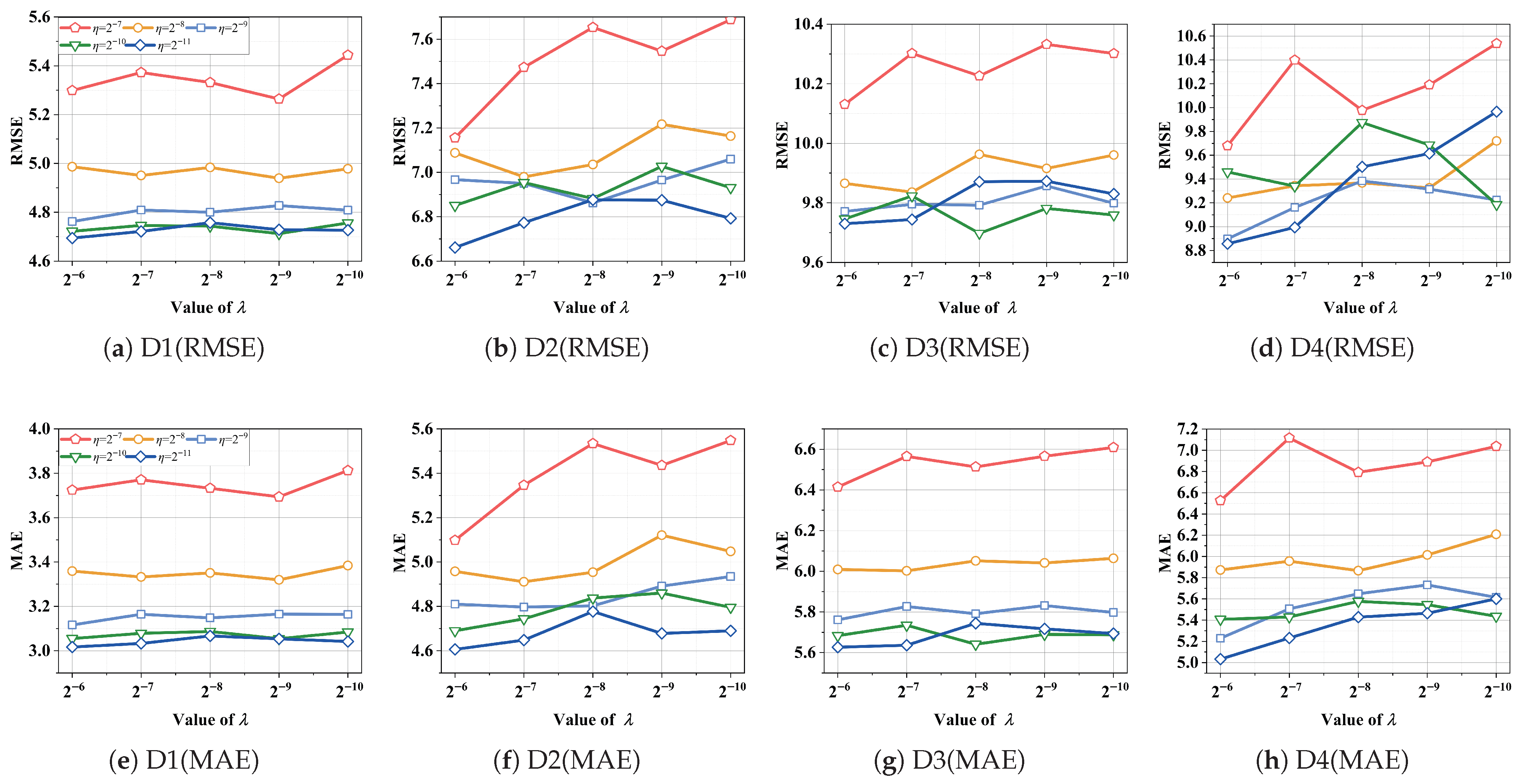
- To evaluate the sensitivity of the Lp,ϵLFT model, we conduct a grid search over the hyper-parameter space: , , , .
5.2. Parameter Sensitivity Test
- 1.
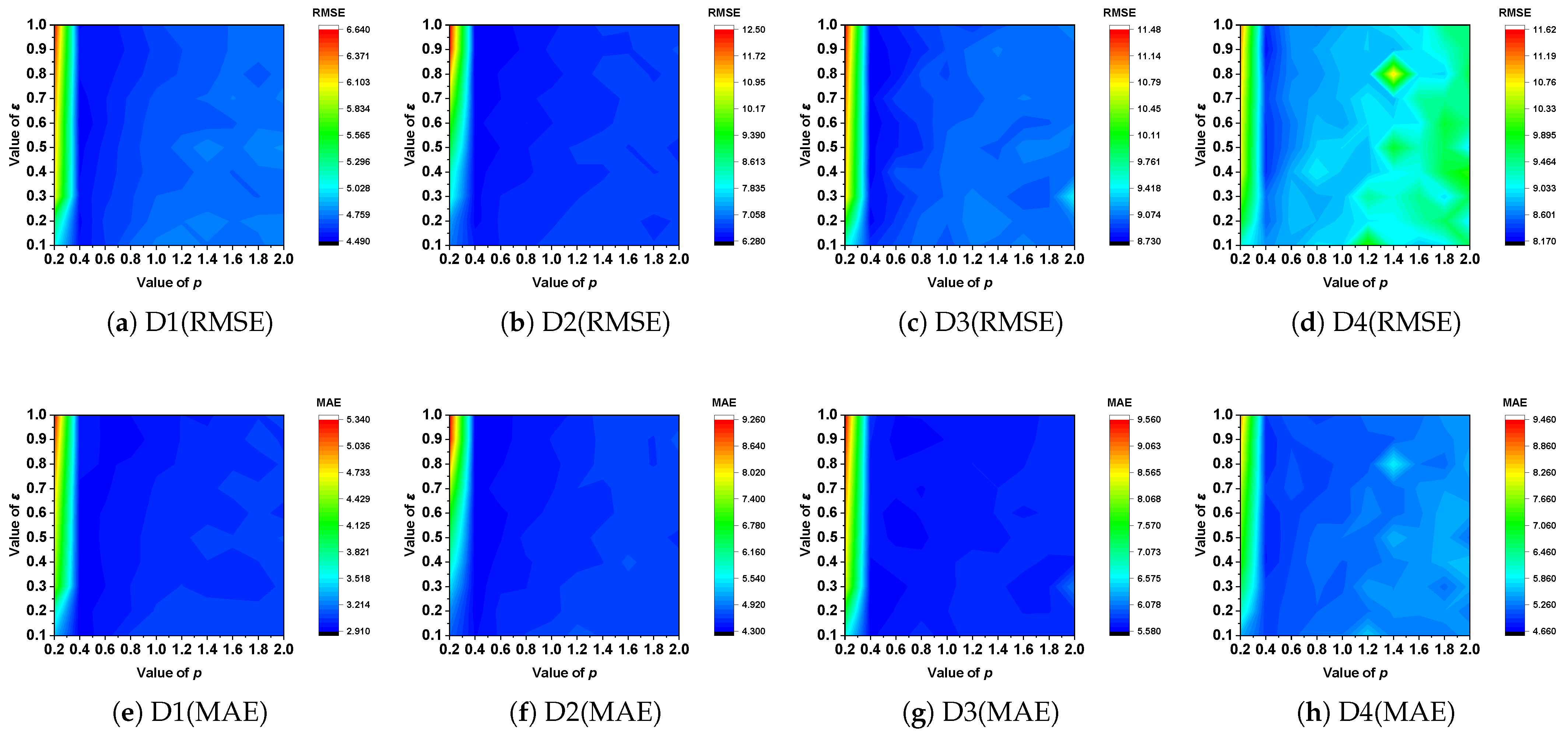
- Be carefully selecting appropriate values for p and , Lp,ϵLFTmanual is able to learn the nonstandard tensor with higher accuracy compared to the commonly adopted L1-norm and L2-norm. As shown in Table 5 and Figure 3c, on D3, Lp,ϵLFTmanual achieves the lowest RMSE of 8.7366 when p = 0.4 and = 0.8. In contrast, the standard L2-norm, achieves an RMSE of 9.1774. Compared with the carefully tuned Lp,ϵ-norm, the performance improvement is 4.80% in terms of RMSE. Analogous phenomena are observed in MAE and across datasets D1-D6. The results show that the Lp,ϵ-norm achieved the lowest value in the F-rank value, confirming the significant advantage of the Lp,ϵ-norm compared to L1/L2-norm, and the results of the signed rank test show that the performance difference between the Lp,ϵ-norm and the L1/L2-norm is statistically significant (p-value < 0.05). These results demonstrate that the Lp,ϵ-norm provides stronger representative capacity compared to the L2-norm when constructing the learning objective of an LFT model.
- 2.
- The optimal depends on the specific dataset. As illustrated in Table 5, when is set to 0.6 on D2, Lp,ϵLFTmanual achieves its lowest RMSE of 6.2802. Meanwhile, the optimal RMSE of 8.7366 is achieved when is adjusted to 0.8 on D3. Moreover, when becomes too small, the nonsmoothness and nonconvexity of the Lp,ϵ-norm pose challenges to optimization.
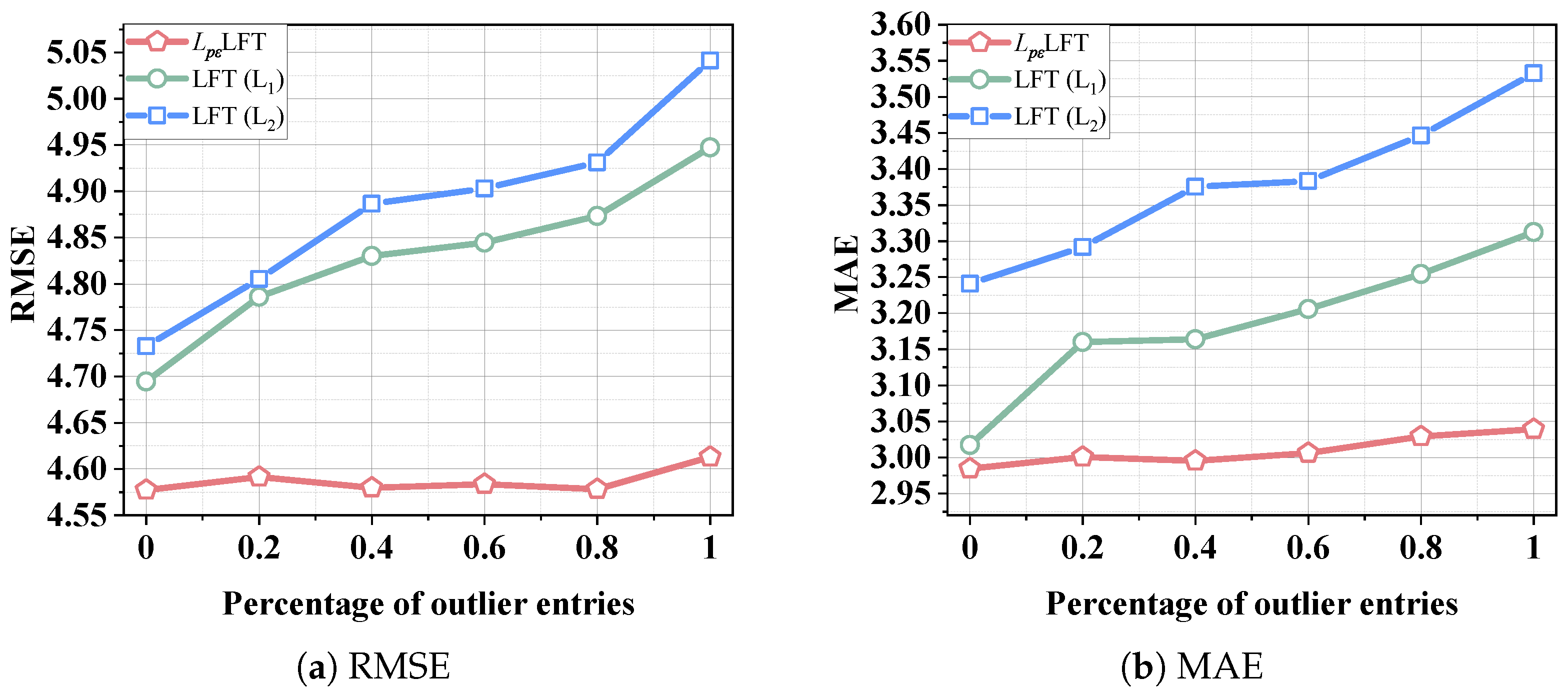
5.3. Outlier Data Sensitivity Test
5.4. Ablation Studies with the Lp,ϵLFT’s Hyper-Parameter Adaption Mechanism
- 1.
- Lp,ϵLFT incorporates a hyper-parameter adaptation mechanism that maintains its representation learning ability for a nonstandard tensor, ensuring no adverse impact on performance. As recorded in Table 7, the RMSE/MAE gap between Lp,ϵLFT and Lp,ϵLFTmanual, (i.e., ()/ and ()/), is almost negligible. Namely, on dataset D1, the RMSE values of Lp,ϵLFT and Lp,ϵLFTmanual are 4.5563 and 4.5627, respectively, corresponding to a gap of 0.14%. Similarly, the MAE values are 2.9907 and 2.9773, respectively, with a gap of 0.44%. It is worth noting that comparable results can be observed across other test cases. Therefore, we can confidently conclude that the hyper-parameter adaptation mechanism in Lp,ϵLFT does not have adverse effects on its representation learning ability.
- 2.
- Self-adaptive hyper-parameters significantly enhance Lp,ϵLFT’s computational efficiency. Notably, the cumulative computational cost of executing the learning model should include the time spent on hyper-parameter tuning to achieve optimal performance. For Lp,ϵLFTmanual, the hyper-parameters p, , , and require a four-fold grid search to determine their optimal values; therefore, the total computational cost comprises the cumulative training time under various hyper-parameter settings. In contrast, for a model employing a hyper-parameters adaptation mechanism, the total computational cost corresponds to a single execution since no explicit hyper-parameter tuning is needed. As shown in Table 7, it is evident that the total computational cost of Lp,ϵLFT is significantly lower than that of Lp,ϵLFTmanual. For example, as displayed in Table 7, on D1, Lp,ϵLFT requires 67 s, which accounts for approximately 0.15% of the 42,500 s required by Lp,ϵLFTmanual in terms of RMSE. Similar results are observed across other datasets.
- 3.
- To summarize, the hyper-parameter adaptation mechanism in Lp,ϵLFT is essential, as it significantly improves efficiency and scalability without compromising representation accuracy.
5.5. Comparison with State-of-the-Art Models
- 1.
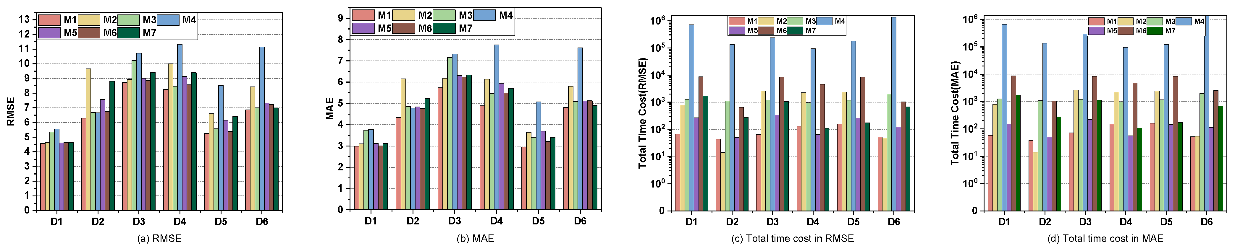
- The proposed Lp,ϵLFT model (referred to as M1) demonstrates superior performance compared to other methods in predicting missing entries within the nonstandard tensor. As illustrated in Figure 6 and summarized in Table 10, M1 consistently achieves the lowest RMSE and MAE on D1–6. Specifically, on D1, M1 attains an RMSE of 4.5563, which is about 1.95% lower than 4.6472 by M2 (RMSEM2-RMSEM1/RMSEM2), 14.87% lower than 5.3524 by M3, 18.08% lower than 5.5620 by M4, 1.23% lower by 4.6131 by M5, 1.67% lower than 4.6340 by M6, and 1.51% lower than 4.6263 by M7. In view of MAE, on D1, the output by M1–7 are 2.9907, 3.1008, 3.7351, 3.7896, 3.1170, 3.0029, and 3.1244, respectively. Consequently, M1’s MAE is also significantly lower compared to that of the other models. Consistent observations are found on D2–D6, with detailed results presented in Table 10 and Figure 6.
- 2.
- The M1 exhibits markedly higher computational performance compared to its peers. When evaluating the time requirements for a learning model to reach optimal performance, it is essential to consider the time cost of hyper-parameter tuning through grid search, particularly in the absence of self-adaptation for parameters. The cost is influenced by the number of hyper-parameters and empirical heuristics. Table 9 presents a summary of the optimal hyper-parameters values for M2–M7 obtained through grid search. As shown in Table 9, the fuzzy controller enables M1 to eliminate the need for grid search, thereby significantly enhancing its computational efficiency. As illustrated in Table 11 and Figure 6, on D1, the total time costs for RMSE and MAE for M1 are 67 and 58 s. These values are the lowest among all models, demonstrating that M1 achieves the lowest RMSE and MAE in a single training run. By comparison, for M6, the empirical range for Cauchy loss is typically [10, 400], and the regularization coefficient is usually [10−1, 10−5]. Obtaining optimally tuned results requires an average of 25 training iterations using a 5 × 5 hyper-parameter grid search. Thus, M6 requires approximately 8725 s to attain the minimum RMSE and MAE, indicating a noticeably greater computational cost compared with M1. Similarly, for D1, M2–M5 and M7 also exhibit higher time consumption in both RMSE and MAE evaluations than M1. This pattern consistently appears across D2–D6, as detailed in Table 11 and illustrated in Figure 6.
- 3.
- The performance gains of M1 are substantial. To further analyze these results, we conduct a Wilcoxon signed-ranks test on the data. This test, a nonparametric method for pairwise comparison, involves three key indicators: R+, R−, and the p-value. A greater R+ coefficient indicates better model performance, while the p-value assesses the statistical significance of the obtained outcomes. The findings of the Wilcoxon signed-rank tests at a 0.1 significance threshold are outlined in Table 12. Note that for Table 10 and Table 11, two distinct cases are considered, with RMSE and MAE as accuracy metrics for each dataset, leading to a total of 12 cases corresponding to 7 models.
5.6. Block-Wise Missing
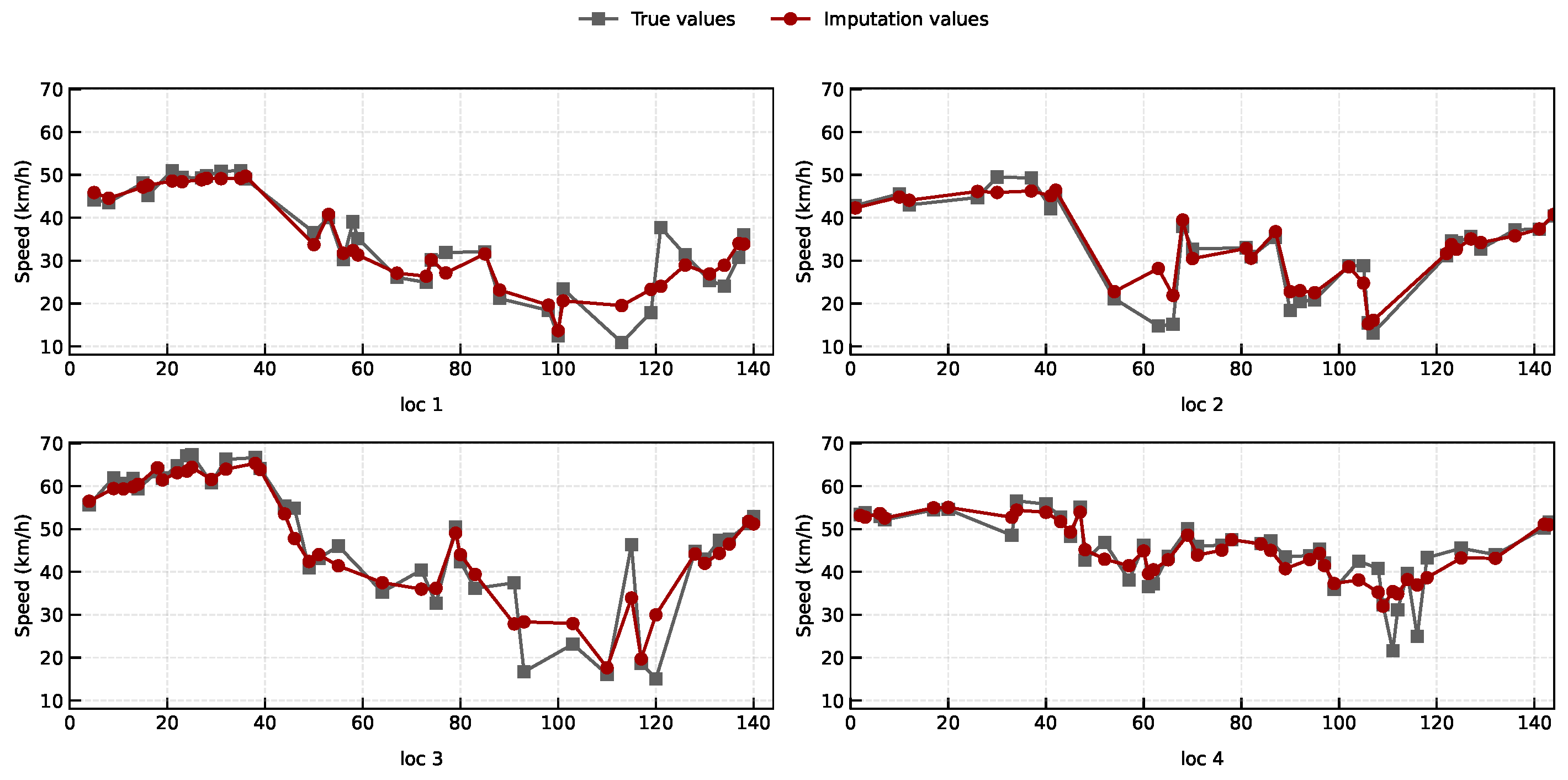
5.7. Case Study
5.8. Summary
- 1.
- It constructs a generalized objective function based on the Lp,ϵ-norm, which robustly represents outliers arising in real-world applications. Additionally, it estimates the LF matrices based on the observed data of the nonstandard tensor, thereby maintaining a computational efficiency that is competitive.
- 2.
- It incorporates an effective adaptation of hyper-parameters using a fuzzy controller, eliminating the need for costly manual tuning, and, thus, ensuring high scalability in real-world scenarios.
6. Conclusions
Author Contributions
Funding
Data Availability Statement
Conflicts of Interest
Appendix A. Comparison Between Lp,ϵ-Norm and Lp-Norm
References
- Wang, J.; Liu, X.; Xu, L.; Li, M.; Li, L.; Shen, S. Local unitary equivalence of quantum states based on the tensor decompositions of unitary matrices. Entropy 2023, 25, 1139. [Google Scholar] [CrossRef]
- Li, X.P.; So, H.C. Robust Low-Rank Tensor Completion Based on Tensor Ring Rank via ℓp,ϵ-Norm. IEEE Trans. Signal Process. 2021, 69, 3685–3698. [Google Scholar] [CrossRef]
- Yang, Z.; Yang, L.T.; Li, C.; Shan, L.; Zhao, H.; Nie, X. Collaborative Bayesian Tensor Factorization-Based Reliable Traffic Speed Data Prediction in T-CPS. IEEE Trans. Intell. Transp. Syst. 2025, 26, 14393–14406. [Google Scholar] [CrossRef]
- Chen, X.; Zhuang, D.; Cai, H.; Wang, S.; Zhao, J. Dynamic Autoregressive Tensor Factorization for Pattern Discovery of Spatiotemporal Systems. IEEE Trans. Pattern Anal. Mach. Intell. 2025, 47, 8524–8537. [Google Scholar] [CrossRef]
- Zhu, Y.; Wang, J.; Wang, J.; He, Z. Multitask neural tensor factorization for road traffic speed-volume correlation pattern learning and joint imputation. IEEE Trans. Intell. Transp. Syst. 2022, 23, 24550–24560. [Google Scholar] [CrossRef]
- Xing, J.; Liu, R.; Anish, K.; Liu, Z. A customized data fusion tensor approach for interval-wise missing network volume imputation. IEEE Trans. Intell. Transp. Syst. 2023, 24, 12107–12122. [Google Scholar] [CrossRef]
- Chen, H.; Lin, M.; Liu, J.; Yang, H.; Zhang, C.; Xu, Z. NT-DPTC: A non-negative temporal dimension preserved tensor completion model for missing traffic data imputation. Inf. Sci. 2024, 653, 119797. [Google Scholar] [CrossRef]
- Zeng, W.J.; So, H.C.; Huang, L. lp-MUSIC: Robust Direction-of-Arrival Estimator for Impulsive Noise Environments. IEEE Trans. Signal Process. 2013, 61, 4296–4308. [Google Scholar] [CrossRef]
- Wu, D.; Zhang, P.; He, Y.; Luo, X. A double-space and double-norm ensembled latent factor model for highly accurate web service QoS prediction. IEEE Trans. Serv. Comput. 2022, 16, 802–814. [Google Scholar] [CrossRef]
- Chen, T.; Yang, W.; Li, S.; Luo, X. An Adaptive p-Norms-Based Kinematic Calibration Model for Industrial Robot Positioning Accuracy Promotion. IEEE Trans. Syst. Man Cybern. Syst. 2025, 55, 2937–2949. [Google Scholar] [CrossRef]
- Zeng, W.J.; So, H.C. Outlier-Robust Matrix Completion via lp-Minimization. IEEE Trans. Signal Process. 2017, 66, 1125–1140. [Google Scholar] [CrossRef]
- Nie, F.; Wang, H.; Cai, X.; Huang, H.; Ding, C. Robust matrix completion via joint schatten p-norm and lp-norm minimization. In Proceedings of the 2012 IEEE 12th International Conference on Data Mining, Brussels, Belgium, 10–13 December 2012; pp. 566–574. [Google Scholar]
- Yang, H.; Lin, M.; Chen, H.; Luo, X.; Xu, Z. Latent factor analysis model with temporal regularized constraint for road traffic data imputation. IEEE Trans. Intell. Transp. Syst. 2025, 26, 724–741. [Google Scholar] [CrossRef]
- Xu, X.; Lin, M.; Luo, X.; Xu, Z. HRST-LR: A hessian regularization spatio-temporal low rank algorithm for traffic data imputation. IEEE Trans. Intell. Transp. Syst. 2023, 24, 11001–11017. [Google Scholar] [CrossRef]
- Sure, P.; Srinivasan, C.P.; Babu, C.N. Spatio-temporal constraint-based low rank matrix completion approaches for road traffic networks. IEEE Trans. Intell. Transp. Syst. 2021, 23, 13452–13462. [Google Scholar] [CrossRef]
- Chen, H.; Lin, M.; Zhao, L.; Xu, Z.; Luo, X. Fourth-order dimension preserved tensor completion with temporal constraint for missing traffic data imputation. IEEE Trans. Intell. Transp. Syst. 2025, 26, 6734–6748. [Google Scholar] [CrossRef]
- Chen, P.; Li, F.; Wei, D.; Lu, C. Low-Rank and Deep Plug-and-Play Priors for Missing Traffic Data Imputation. IEEE Trans. Intell. Transp. Syst. 2025, 26, 2690–2706. [Google Scholar] [CrossRef]
- Baggag, A.; Abbar, S.; Sharma, A.; Zanouda, T.; Al-Homaid, A.; Mohan, A.; Srivastava, J. Learning spatiotemporal latent factors of traffic via regularized tensor factorization: Imputing missing values and forecasting. IEEE Trans. Knowl. Data Eng. 2019, 33, 2573–2587. [Google Scholar] [CrossRef]
- Shu, H.; Wang, H.; Peng, J.; Meng, D. Low-rank tensor completion with 3-D spatiotemporal transform for traffic data imputation. IEEE Trans. Intell. Transp. Syst. 2024, 25, 18673–18687. [Google Scholar] [CrossRef]
- Wei, X.; Zhang, Y.; Wang, S.; Zhao, X.; Hu, Y.; Yin, B. Self-attention graph convolution imputation network for spatio-temporal traffic data. IEEE Trans. Intell. Transp. Syst. 2024, 25, 19549–19562. [Google Scholar] [CrossRef]
- Zhang, K.; Zhou, F.; Wu, L.; Xie, N.; He, Z. Semantic understanding and prompt engineering for large-scale traffic data imputation. Inf. Fusion 2024, 102, 102038. [Google Scholar] [CrossRef]
- Wang, S.; Li, J.; Miao, H.; Zhang, J.; Zhu, J.; Wang, J. Generative-free urban flow imputation. In Proceedings of the 31st ACM International Conference on Information & Knowledge Management, Atlanta, GA, USA, 17–21 October 2022; pp. 2028–2037. [Google Scholar]
- Zhang, Y.; Wei, X.; Zhang, X.; Hu, Y.; Yin, B. Self-attention graph convolution residual network for traffic data completion. IEEE Trans. Big Data 2022, 9, 528–541. [Google Scholar] [CrossRef]
- Xu, D.; Peng, H.; Tang, Y.; Guo, H. Hierarchical spatio-temporal graph convolutional neural networks for traffic data imputation. Inf. Fusion 2024, 106, 102292. [Google Scholar] [CrossRef]
- Wu, D.; Li, Z.; Yu, Z.; He, Y.; Luo, X. Robust low-rank latent feature analysis for spatiotemporal signal recovery. IEEE Trans. Neural Netw. Learn. Syst. 2023, 36, 2829–2842. [Google Scholar] [CrossRef]
- Wu, D.; Luo, X. Robust latent factor analysis for precise representation of high-dimensional and sparse data. IEEE/CAA J. Autom. Sin. 2020, 8, 796–805. [Google Scholar] [CrossRef]
- Liu, S.; Shi, X.; Liao, Q. Rank-adaptive tensor completion based on Tucker decomposition. Entropy 2023, 25, 225. [Google Scholar] [CrossRef]
- Favier, G.; Rocha, D.S. Overview of Tensor-Based Cooperative MIMO Communication Systems—Part 2: Semi-Blind Receivers. Entropy 2024, 26, 937. [Google Scholar] [CrossRef] [PubMed]
- Jørgensen, P.J.; Nielsen, S.F.; Hinrich, J.L.; Schmidt, M.N.; Madsen, K.H.; Mørup, M. Probabilistic parafac2. Entropy 2024, 26, 697. [Google Scholar] [CrossRef]
- Huang, X.; Chen, D.; Wang, D.; Ren, T. Identifying influencers in social networks. Entropy 2020, 22, 450. [Google Scholar] [CrossRef] [PubMed]
- Zeng, J.; Qiu, Y.; Ma, Y.; Wang, A.; Zhao, Q. A novel tensor ring sparsity measurement for image completion. Entropy 2024, 26, 105. [Google Scholar] [CrossRef] [PubMed]
- Wu, D.; Hu, Y.; Liu, K.; Li, J.; Wang, X.; Deng, S.; Zheng, N.; Luo, X. An Outlier-Resilient Autoencoder for Representing High-Dimensional and Incomplete Data. IEEE Trans. Neural Netw. Learn. Syst. 2025, 9, 1379–1391. [Google Scholar] [CrossRef]
- Chen, X.; Sun, L. Bayesian temporal factorization for multidimensional time series prediction. IEEE Trans. Pattern Anal. Mach. Intell. 2021, 44, 4659–4673. [Google Scholar] [CrossRef] [PubMed]
- Liu, M.; Huang, H.; Feng, H.; Sun, L.; Du, B.; Fu, Y. Pristi: A conditional diffusion framework for spatiotemporal imputation. In Proceedings of the 2023 IEEE 39th International Conference on Data Engineering, Anaheim, CA, USA, 3–7 April 2023; pp. 1927–1939. [Google Scholar]
- Luo, X.; Wu, H.; Li, Z. NeuLFT: A novel approach to nonlinear canonical polyadic decomposition on high-dimensional incomplete tensors. IEEE Trans. Knowl. Data Eng. 2022, 35, 6148–6166. [Google Scholar] [CrossRef]
- Che, H.; Pan, B.; Leung, M.F.; Cao, Y.; Yan, Z. Tensor factorization with sparse and graph regularization for fake news detection on social networks. IEEE Trans. Comput. Social Syst. 2023, 11, 4888–4898. [Google Scholar] [CrossRef]
- Yuan, S.; Huang, K. A generalizable framework for low-rank tensor completion with numerical priors. Pattern Recognit. 2024, 155, 110678. [Google Scholar] [CrossRef]
- Tao, Z.; Tanaka, T.; Zhao, Q. Efficient nonparametric tensor decomposition for binary and count data. In Proceedings of the AAAI Conference on Artificial Intelligence; AAAI Press: Vancouver, BC, Canada, 2024; Volume 38, pp. 15319–15327. [Google Scholar]
- Luo, X.; Wu, H.; Yuan, H.; Zhou, M. Temporal pattern-aware QoS prediction via biased non-negative latent factorization of tensors. IEEE Trans. Cybern. 2019, 50, 1798–1809. [Google Scholar] [CrossRef] [PubMed]
- Ye, F.; Lin, Z.; Chen, C.; Zheng, Z.; Huang, H. Outlier-resilient web service QoS prediction. In Proceedings of the Web Conference 2021, Ljubljana, Slovenia, 19–23 April 2021; pp. 3099–3110. [Google Scholar]
- Su, X.; Zhang, M.; Liang, Y.; Cai, Z.; Guo, L.; Ding, Z. A tensor-based approach for the QoS evaluation in service-oriented environments. IEEE Trans. Netw. Serv. Manag. 2021, 18, 3843–3857. [Google Scholar] [CrossRef]



| Symbol | Description |
|---|---|
| Number of sensors, time intervals, and days, respectively. | |
| Real number domain. | |
| Original incomplete data tensor from ITS. | |
| Low-rank approximation to . | |
| A third-order latent factor tensor. | |
| The k-th frontal slice of . | |
| Latent factor matrices. | |
| A single element in , , . | |
| The ith, jth and kth row vectors of , , . | |
| Single entries in , , . | |
| R | The dimension of latent factor space. |
| ∘ | Outer product of two vectors. |
| ⊙ | Hadamard product of two vectors. |
| Frobenius norm of a tensor. | |
| Cardinality of an enclosed set. | |
| Learning rate. | |
| Regularization coefficient. | |
| The subsets of known entry set related to entities | |
| Training, validation and testing sets from . |
| p | ||||
|---|---|---|---|---|
| No. | Dataset | Sensor Count | Time Slots | Day Count | Known Entries |
|---|---|---|---|---|---|
| D1 | Guangzhou | 214 | 144 | 61 | 92,779 |
| D2 | Seattle | 20,833 | 24 | 31 | 70,528 |
| D3 | New York | 135 | 288 | 73 | 109,651 |
| D4 | Metr-la | 207 | 288 | 119 | 65,190 |
| D5 | Pems-bay | 325 | 288 | 181 | 84,685 |
| D6 | Berlin | 12,416 | 24 | 31 | 138,999 |
| p | ||||
|---|---|---|---|---|
| 1 | ||||
| No. | Optimal p and | EMSE | RMSE () | RMSE () |
|---|---|---|---|---|
| D1 | 4.5627 | 4.6946 | 4.7327 | |
| D2 | 6.2802 | 6.6612 | 6.6074 | |
| D3 | 8.7366 | 9.6978 | 9.1774 | |
| D4 | 8.2733 | 8.8564 | 9.2885 | |
| D5 | 5.2792 | 5.5320 | 6.1070 | |
| D6 | 6.8552 | 7.1036 | 6.9729 | |
| Statistic | win/loss | 6/0 | 0/6 | 0/6 |
| F-rank | 1.00 | 2.50 | 2.50 | |
| p-value | - | 0.0156 | 0.0156 |
| No. | Optimal p and | MAE | MAE () | MAE () |
|---|---|---|---|---|
| D1 | 2.9773 | 3.0172 | 3.2409 | |
| D2 | 4.3067 | 4.6066 | 4.7001 | |
| D3 | 5.7432 | 5.6411 | 6.4518 | |
| D4 | 4.8907 | 5.0968 | 6.2254 | |
| D5 | 2.9584 | 3.0126 | 3.8430 | |
| D6 | 4.8499 | 4.9308 | 5.0583 | |
| Statistic | win/loss | 5/1 | 1/5 | 0/6 |
| F-rank | 1.17 | 1.83 | 3.00 | |
| p-value | - | 0.1094 | 0.0156 |
| Datasets | Metrics | Lp,ϵLFT | Lp,ϵLFTmanual |
|---|---|---|---|
| D1 | RMSE | 4.5563±1.24 × 10⁻² | 4.5627±1.48 × 10⁻² |
| Time-RMSE | 67±14 | 42,500±8 | |
| MAE | 2.9907±1.46 × 10⁻² | 2.9773±9.50 × 10⁻³ | |
| Time-MAE | 58±10 | 47,500±10 | |
| D2 | RMSE | 6.2902±3.81 × 10⁻² | 6.3532±7.90 × 10⁻² |
| Time-RMSE | 43±2.19 | 26,875±7.42 | |
| MAE | 4.3322±1.66 × 10⁻² | 4.3483±1.12 × 10⁻² | |
| Time-MAE | 38±1.49 | 26,875±5.13 | |
| D3 | RMSE | 8.7279 ±2.61 × 10⁻² | 8.7366±1.51 × 10⁻² |
| Time-RMSE | 66±3.58 | 37,500±5.49 | |
| MAE | 5.7348±7.55 × 10⁻³ | 5.7432±4.99 × 10⁻³ | |
| Time-MAE | 72±8.56 | 53,125±5.80 | |
| D4 | RMSE | 8.2548±3.83 × 10⁻² | 8.2733±3.22 × 10⁻² |
| Time-RMSE | 132±12.56 | 63,750±15 | |
| MAE | 4.8916±1.95 × 10⁻² | 4.8907±1.52 × 10⁻² | |
| Time-MAE | 149±10.43 | 72,500±4 | |
| D5 | RMSE | 5.2565±2.75 × 10⁻² | 5.2792±1.65 × 10⁻² |
| Time-RMSE | 162±10 | 95,000±2.21 | |
| MAE | 2.9560±2.26 × 10⁻² | 2.9584±2.99 × 10⁻² | |
| Time-MAE | 162±10 | 96,875±0.14 | |
| D6 | RMSE | 6.8597±3.05 × 10⁻³ | 6.8552±2.27 × 10⁻² |
| Time-RMSE | 52±4.65 | 135,000±6.29 | |
| MAE | 4.8122±1.05 × 10⁻² | 4.8499±6.44 × 10⁻³ | |
| Time-MAE | 53±4.39 | 128,125±7.20 |
| No. | Model | Description | Hyper-Parameter |
|---|---|---|---|
| M1 | Lp,ϵLFT | The proposed model developed in this study. | Self-adaptation |
| M2 | SGCP | A learning framework employing a sparse and graph constraint within a canonical polyadic (CP) tensor decomposition structure [36]. | , sparse regularization , graph regularization |
| M3 | SPTC | A smooth Poisson tensor completion algorithm that generalizes CP decomposition and incorporates the numerical priors of the data [37]. | , smoothing coefficient , learning rate |
| M4 | ENTED | An effective nonparametric tensor decomposition approach that utilizes a Gaussian process along with Pólya-Gamma augmentation to form conjugate models [38]. | p, number of inducing points , number of successes , learning rate M, batch size |
| M5 | BNLFT | A biased non-negative latent factorization of tensors for time-aware prediction [39]. | , regularization parameter |
| M6 | CTF | A method based on CP decomposition, where the Cauchy loss function is used to quantify the difference between observed and predicted values [40]. | , Cauchy loss , regularization coefficient |
| M7 | TCA | A reverse CP decomposition method that updates all factor matrices using either alternating least squares or gradient descent techniques [41]. | , regularization coefficient , learning rate |
| Dataset | Hyper-Parameter Setting |
|---|---|
| D1 | M1: Self-adaptive M2: = 1, = 1 M3: = 1×10⁻⁴, = 10 M4: p = 30, = 10, = 0.01, M = 64 M5: = 0.1, = 0.1 M6: = 10, = 10−3 M7: = 10−5, = 10−2 |
| D2 | M1: Self-adaptation M2: = 1, = 10 M3: = 1×10⁻⁴, = 50 M4: p = 10, = 30, = 0.01, M = 64 M5: = 1, = 10−6 M6: = 10, = 10−2 M7: = 10−5, = 10−5 |
| D3 | M1: Self-adaptation M2: = 1, = 1000 M3: = 1×10⁻⁴, = 70 M4: p = 10, = 50, = 0.01, M = 128 M5: = 0.1, = 0.1 M6: = 200, = 10−5 M7: = 10−5, = 10−1 |
| D4 | M1: Self-adaptive M2: = 0.1, = 1000 M3: = 1×10⁻³, = 10 M4: p = 10, = 30, = 0.01, M = 64 M5: = 1, = 10−4 M6: = 300, = 10−5 M7: = 10−4, = 10−1 |
| D5 | M1: Self-adaptive M2: = 1, = 1000 M3: = 1×10⁻³, = 10 M4: p = 30, = 50, = 0.01, M = 128 M5 = 0.1, = 10−5 M6: = 200, = 10−5 M7: = 10−4, = 10−1 |
| D6 | M1: Self-adaptive M2: = 1, = 10 M3: = 1×10⁻⁴, = 30 M4: p = 30, = 10, = 0.01, M = 64 M5: = 1, = 10−3 M6: = 300, = 10−5 M7: = 10−5, = 10−2 |
| Case | M1 | M2 | M3 | M4 | M5 | M6 | M7 | Gains vs. Best | |
|---|---|---|---|---|---|---|---|---|---|
| D1 | RMSE | 4.5563±1.24 × 10⁻² | 4.6472±2.06 × 10⁻² | 5.3524±2.10 × 10⁻² | 5.5620±0 | 4.6131±1.73 × 10⁻² | 4.6340±6.21 × 10⁻³ | 4.6263±1.04 × 10⁻² | 1.23% |
| MAE | 2.9907±1.46 × 10⁻² | 3.1008±1.38 × 10⁻² | 3.7351±2.41 × 10⁻² | 3.7896±0 | 3.1170±1.47 × 10⁻² | 3.0029±4.05 × 10⁻³ | 3.1244±6.07 × 10⁻³ | 0.41% | |
| D2 | RMSE | 6.2902±3.81 × 10⁻² | 9.6501±2.00 × 10⁻¹ | 6.6815±1.91 × 10⁻¹ | 6.6626±0 | 7.5726±3.81 × 10⁻² | 6.7513±1.54 × 10⁻² | 8.8178±2.96 × 10⁻³ | 5.59% |
| MAE | 4.3322±1.66 × 10⁻³ | 6.1528±1.60 × 10⁻¹ | 4.8513±1.53 × 10⁻¹ | 4.7785±0 | 4.8338±2.54 × 10⁻² | 4.7716±1.88 × 10⁻² | 5.2233±4.55 × 10⁻⁴ | 9.21% | |
| D3 | RMSE | 8.7279±2.61 × 10⁻² | 8.9452±2.27 × 10⁻² | 10.2218±1.35 × 10⁻¹ | 10.7175±0 | 9.0236±3.44 × 10⁻² | 8.8570±1.14 × 10⁻² | 9.4179±3.88 × 10⁻² | 1.46% |
| MAE | 5.7348±7.55 × 10⁻³ | 6.1897±6.79 × 10⁻³ | 7.1542±2.20 × 10⁻¹ | 7.3256±0 | 6.3108±3.42 × 10⁻² | 6.2360±1.51 × 10⁻² | 6.3332±1.56 × 10⁻² | 7.89% | |
| D4 | RMSE | 8.2548±4.17 × 10⁻² | 10.0005±5.30 × 10⁻² | 8.4697±2.15 × 10⁻² | 11.3228±0 | 9.1325±1.60 × 10⁻¹ | 8.5762±4.38 × 10⁻² | 9.3954±4.26 × 10⁻² | 2.54% |
| MAE | 4.8916±4.34 × 10⁻² | 6.1495±4.74 × 10⁻² | 5.4630±1.05 × 10⁻² | 7.7476±0 | 5.9487±7.74 × 10⁻² | 5.4852±4.94 × 10⁻² | 5.7196±4.18 × 10⁻² | 10.46% | |
| D5 | RMSE | 5.2565±2.75 × 10⁻² | 6.6003±3.45 × 10⁻² | 5.5713±3.00 × 10⁻² | 8.5231±0 | 6.1571±1.65 × 10⁻² | 5.3868±2.81 × 10⁻² | 6.4094±4.36 × 10⁻² | 2.42% |
| MAE | 2.9560±2.26 × 10⁻² | 3.6441±2.27 × 10⁻² | 3.4066±2.04 × 10⁻² | 5.0772±0 | 3.7010±8.07 × 10⁻³ | 3.2087±2.66 × 10⁻² | 3.4008±6.07 × 10⁻² | 7.87% | |
| D6 | RMSE | 6.8597±3.05 × 10⁻² | 8.4374±1.98 × 10⁻² | 7.0087±2.49 × 10⁻² | 11.1509±0 | 7.3273±4.76 × 10⁻² | 7.2214±3.25 × 10⁻² | 6.9866±7.33 × 10⁻³ | 1.82% |
| MAE | 4.8122±1.05 × 10⁻² | 5.8063±2.66 × 10⁻² | 5.0891±2.26 × 10⁻² | 7.6089±0 | 5.1150±3.99 × 10⁻² | 5.1257±1.34 × 10⁻² | 4.9100±8.73 × 10⁻³ | 1.99% | |
| Case | M1 | M2 | M3 | M4 | M5 | M6 | M7 | |
|---|---|---|---|---|---|---|---|---|
| D1 | Time-RMSE | 67±14 | 786±0.78 | 1275±4.55 | 721,875±45 | 273 ±1.38 | 8725±16.74 | 1700±1.94 |
| Time-MAE | 58±10 | 798±0.83 | 1275±4.55 | 664,375±43 | 151±1.03 | 8725±16.74 | 1700±1.86 | |
| D2 | Time-RMSE | 43±2.19 | 14±8.11 × 10⁻² | 1100±3.46 | 135,000±10 | 50±0.79 | 650±6.79 | 275±0.53 |
| Time-MAE | 38±1.49 | 14±8.38 × 10⁻² | 1100±3.46 | 135,000±10 | 50±0.79 | 1050±15.12 | 275±0.47 | |
| D3 | Time-RMSE | 66±3.58 | 2632±1.49 | 1200±2.87 | 239,375±28 | 341±2.96 | 8375±2.07 | 1075±2.41 |
| Time-MAE | 72±8.56 | 2677±0.94 | 1200±2.87 | 290,000±41 | 224±1.91 | 8375±2.07 | 1125±2.59 | |
| D4 | Time-RMSE | 132±10.81 | 2240±5.34 | 975±3.44 | 95,000±34 | 66±2.28 | 4625±9.00 | 111±0.20 |
| Time-MAE | 149±9 | 2245±5.34 | 975±3.44 | 95,000±34 | 57±2.60 | 4750±9.40 | 109±0.21 | |
| D5 | Time-RMSE | 162±10 | 2400±0.83 | 1175±1.48 | 181,250±24 | 263±0.30 | 8400±0.58 | 178±0.32 |
| Time-MAE | 162±10 | 2408±0.83 | 1175±1.48 | 122,500±31 | 145±1.24 | 8400±0.58 | 172±0.20 | |
| D6 | Time-RMSE | 52±4.65 | 49±5.65 | 2000±2.87 | 1,323,750±24 | 121±0.10 | 1050±3.17 | 675±1.68 |
| Time-MAE | 53±4.39 | 54±8.03 | 2000±2.87 | 1,323,750±24 | 114±0.27 | 2575±33.61 | 700±1.71 | |
| Comparison | Accuracy | Efficiency | ||||
|---|---|---|---|---|---|---|
| R+ | R− | p-Value | R+ | R− | p-Value | |
| M1 vs. M2 | 78 | 0 | 0.0002 | 69 | 9 | 0.0080 |
| M1 vs. M3 | 78 | 0 | 0.0002 | 78 | 0 | 0.0002 |
| M1 vs. M4 | 78 | 0 | 0.0002 | 78 | 0 | 0.0002 |
| M1 vs. M5 | 78 | 0 | 0.0002 | 63 | 15 | 0.0319 |
| M1 vs. M6 | 78 | 0 | 0.0002 | 78 | 0 | 0.0002 |
| M1 vs. M7 | 78 | 0 | 0.0002 | 71 | 7 | 0.0046 |
| Missing Rate | M1 | M2 | M3 | M4 | M5 | M6 | M7 | |
|---|---|---|---|---|---|---|---|---|
| 0.3 | RMSE | 4.6052 | 4.7912 | 5.5672 | 5.5936 | 4.7043 | 4.6694 | 4.7248 |
| MAE | 2.9845 | 3.2276 | 3.9178 | 3.8178 | 3.1997 | 3.0387 | 3.1974 | |
| 0.5 | RMSE | 4.6830 | 4.9424 | 5.7674 | 6.8441 | 4.8746 | 4.7645 | 4.8171 |
| MAE | 3.0316 | 3.3052 | 4.1162 | 4.9200 | 3.3273 | 3.1243 | 3.2609 | |
| 0.7 | RMSE | 4.7804 | 5.1971 | 5.9281 | 5.6191 | 5.0841 | 4.8587 | 4.9203 |
| MAE | 3.1496 | 3.5681 | 4.2584 | 3.8087 | 3.5056 | 3.2218 | 3.3343 | |
| Statistic | win/loss | 6/0 | 0/6 | 0/6 | 0/6 | 0/6 | 0/6 | 0/6 |
| F-rank | 1.000 | 4.833 | 6.500 | 6.500 | 4.000 | 2.000 | 3.167 | |
| p-value | – | 0.0156 | 0.0156 | 0.0156 | 0.0156 | 0.0156 | 0.0156 | |
Disclaimer/Publisher’s Note: The statements, opinions and data contained in all publications are solely those of the individual author(s) and contributor(s) and not of MDPI and/or the editor(s). MDPI and/or the editor(s) disclaim responsibility for any injury to people or property resulting from any ideas, methods, instructions or products referred to in the content. |
© 2026 by the authors. Licensee MDPI, Basel, Switzerland. This article is an open access article distributed under the terms and conditions of the Creative Commons Attribution (CC BY) license.
Share and Cite
Yang, L.; Ma, Z.; Hou, Y. High-Quality Representation Learning Approach to Spatio-Temporal Traffic Speed Data with Lp,ϵ-Norm. Entropy 2026, 28, 435. https://doi.org/10.3390/e28040435
Yang L, Ma Z, Hou Y. High-Quality Representation Learning Approach to Spatio-Temporal Traffic Speed Data with Lp,ϵ-Norm. Entropy. 2026; 28(4):435. https://doi.org/10.3390/e28040435
Chicago/Turabian StyleYang, Lei, Ziwen Ma, and Yikai Hou. 2026. "High-Quality Representation Learning Approach to Spatio-Temporal Traffic Speed Data with Lp,ϵ-Norm" Entropy 28, no. 4: 435. https://doi.org/10.3390/e28040435
APA StyleYang, L., Ma, Z., & Hou, Y. (2026). High-Quality Representation Learning Approach to Spatio-Temporal Traffic Speed Data with Lp,ϵ-Norm. Entropy, 28(4), 435. https://doi.org/10.3390/e28040435