The experiments in
Section 4.1 and
Section 4.2 and the first part of
Section 4.3 involve training diffusion models using both energy and score parameterizations. The score parameterization follows a noise prediction model,
, while the energy parameterization defines an energy function as
, as in [
18]. We use identical network architectures for
and
. Both models are trained with the standard diffusion loss [
3], with the energy model’s score function obtained through explicit differentiation.
The later experiments utilize only pre-trained score-based diffusion models, as pre-trained energy-based models are unavailable for direct comparison. We evaluate both unadjusted and MH-corrected versions of Langevin and Hamiltonian Monte Carlo, comparing them against the standard reverse process, which serves as the baseline.
For the MH-like correction, we examine two types of integration paths: a straight line between and (Algorithm 2) and the trajectory defined by the HMC leapfrog steps (Algorithm 3). Both approaches rely on a trapezoidal rule where the number of intermediate points is treated as a hyperparameter.
4.1. Evaluating Pseudo-Energy Differences
To evaluate the accuracy of pseudo-energy differences, we conducted experiments on a synthetic 2D dataset, generated from a bivariate Gaussian distribution to allow access to analytical solutions, and a higher-dimensional dataset, MNIST [
34]. For each experiment, we trained 10 independent score models and 10 independent energy models from scratch. For evaluation, we sampled 2000 pairs of points
independently via the forward process at various diffusion steps
t. These pairs were used to compute the score-based pseudo-energy difference (
) and the explicit EBM energy difference (
), as well as the analytical difference (
) when available. The pseudo-energy difference was computed along a straight-line path connecting the two points, using five discretization points for the numerical integration.
2D Gaussian: For the 2D Gaussian dataset, the relative error metric is defined as , where corresponds to either the explicitly predicted difference from the energy model () or the pseudo-energy difference from the score model (), and is the analytical energy difference. The median relative error was calculated across all sampled pairs for each trained model, and the mean and standard deviation of this metric were computed across the 10 models. Interestingly, the score model achieved a lower relative error () compared to the energy model (), demonstrating that the line-integral approximation aligns slightly better with the true energy differences in this setting.
MNIST: For the MNIST dataset, where analytical energy differences are unavailable, we used a symmetric relative discrepancy metric defined as . The median relative discrepancy was calculated across all sampled pairs for each trained model, and the mean and standard deviation were computed across the 10 models. This yielded a mean symmetric relative discrepancy of , indicating that the pseudo-energy differences predicted by the score models align closely with the explicit EBM predictions, even in this higher-dimensional setting.
4.2. Two-Dimensional Composition
To investigate the effectiveness of our MH-like correction in a controlled yet expressive setting, we replicate the 2D composition experiment introduced by Du et al. [
18] using their publicly available codebase (
https://github.com/yilundu/reduce_reuse_recycle, accessed on 4 January 2025) as a foundation. Only minor modifications are necessary, ensuring a faithful reproduction of their setup. Apart from differences in evaluation metrics, our setup is identical to theirs.
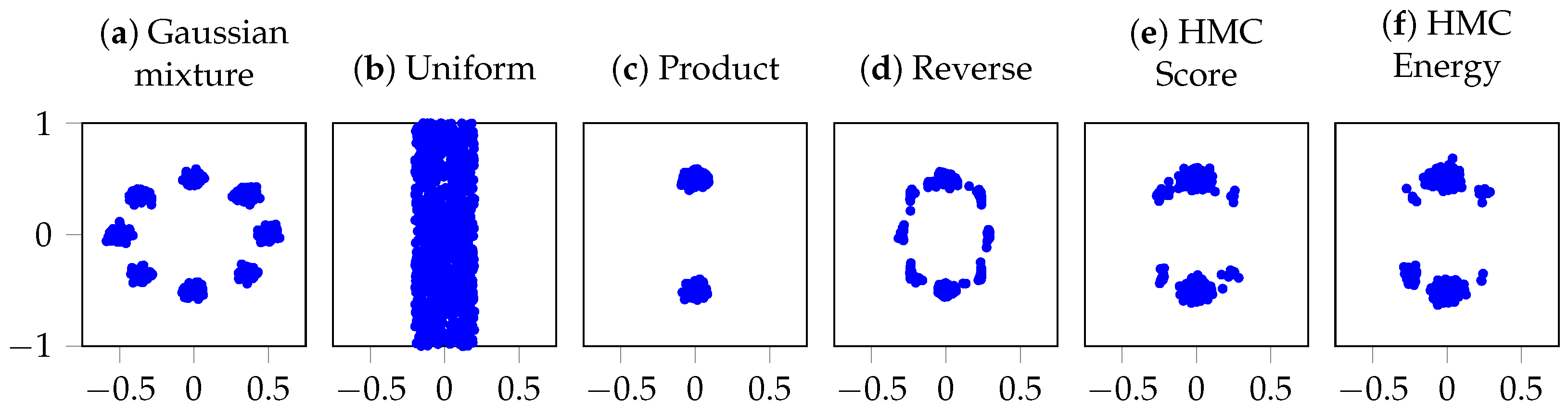
A 2D density pair is composed via multiplication into a complex distribution, as in (
9): a Gaussian mixture with eight modes in a circle and a uniform distribution covering two of the modes. For a visual representation of the two individual distributions and their resulting product distribution together with samples from the reverse diffusion and HMC corrected samples, see
Figure 1. The baseline reverse diffusion process uses
steps. In the MCMC variants, following [
18], we omit the optional reverse step for a fair comparison. MCMC sampling runs for
at each
t, with (U-)HMC using three leapfrog steps per MCMC step.
We evaluate performance using three metrics: (1) negative log-likelihood (NLL), (2) a Gaussian mixture model (GMM) comparison, and (3) the Wasserstein-2 distance (
). The suffixes in
Table 1 refer to the choice of integration path and the number of evaluation points: “L” denotes the straight-line path from Algorithm 2, while “C” denotes the curve path from Algorithm 3. The number indicates trapezoidal evaluation points (
m or
n).
Table 1 reports performance metrics averaged over 10 independent trials. In each trial, we train the diffusion models from scratch and sample 2000 points using different MCMC methods. The corrected sampling methods consistently outperform the unadjusted ones. HMC variants yield the best results across all metrics. Score- and energy-parameterized samplers show similar NLL and GMM performance, while HMC with score parameterization achieves a substantially lower
. Performance also saturates with as few as three integration points.
In addition to performance, we measure runtime and memory consumption. These results are reported separately in
Table 2. The experiment is implemented in JAX (v0.4.30) [
35] and run on a desktop computer equipped with an NVIDIA GeForce RTX 3060 GPU. Score-based parameterization is more than twice as memory-efficient as energy-based parameterization, and—except for LA with
—also faster for corresponding MCMC methods. Notably, the HMC curve variant is significantly faster. Although score-based corrections require more model evaluations, they do not necessarily incur higher runtime or memory costs.
As discussed by Du et al. [
18], directly adding score functions does not yield a valid product composition, which explains why the reverse sampler performs poorly in this setting. This apparent failure is expected and highlights the motivation for annealed MCMC: by treating intermediate distributions as design choices that guide the chain toward the target, annealing achieves improved results while preserving asymptotic correctness. This accounts for the large gap between the reverse method and the annealed MCMC variants reported in
Table 1.
4.3. Guided Diffusion
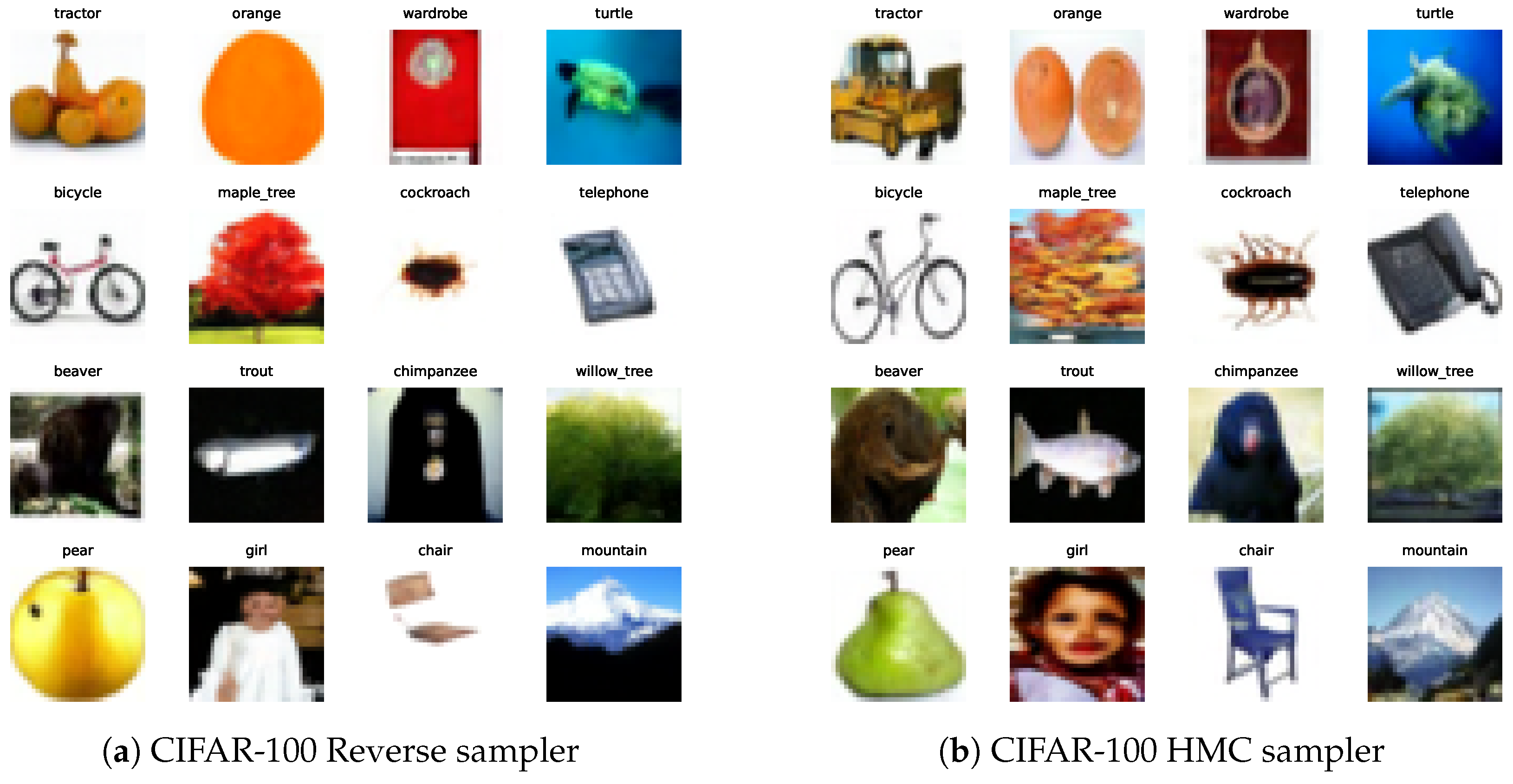
We evaluate our proposed sampling methods for guided diffusion on the CIFAR-100 [
36] and ImageNet [
37] datasets. The sampling process is based on a score function defined in (
7). For both datasets, the marginal score,
, is estimated using an unconditional diffusion model parameterized by a UNet architecture. For the guidance model, we use classifier-full guidance, training a time-dependent classifier to predict class labels across all diffusion steps,
. This classifier shares its architecture with the encoder part of the UNet used for the diffusion model and is extended with a dense output layer. The guidance scale is set to
across all experiments, which is a commonly used default in classifier-guided diffusion models. This choice is also consistent with the settings provided in the public implementation of [
18] (
https://github.com/yilundu/reduce_reuse_recycle, accessed on 4 January 2025). Sampling is based on the standard reverse process with
, and additional MCMC steps are incorporated to refine the generated samples. The
Reverse baseline reported in the tables corresponds to the standard classifier-full guided reverse diffusion process without any additional MCMC refinement steps.
To quantify generation quality, we use three evaluation metrics: the Fréchet Inception Distance (FID) [
38], which compares the distribution of generated and real images; classification accuracy, based on a separate pre-trained classifier applied to generated samples; and, for ImageNet, an additional top 5 accuracy metric.
CIFAR-100: For CIFAR-100, we trained the diffusion models from scratch using the same UNet architecture and training settings as in [
3], which were originally designed for CIFAR-10 [
36]. The MCMC samplers add
or 6 extra MCMC steps at each diffusion step
t for (U-)HMC and (U-)LA, respectively, with (U-)HMC using three leapfrog steps per MCMC step, following the configuration used by Du et al. [
18] in their guided diffusion experiments.
For this experiment, we used denser meshes in the trapezoidal rule compared to the 2D setting. For HMC, we followed the curve defined by the leapfrog steps (Algorithm 3) and set , i.e., the leapfrog points plus an additional midpoint evaluation. For LA, we followed the straight line path (Algorithm 2) with evenly spaced points, corresponding to eight additional evaluations per step.
Recognizing the impact of the step length on MCMC methods, we followed Du et al. [
18] by parameterizing it as a function of the beta-schedule. For Langevin dynamics, the stepsize is given by
, and for HMC, the leapfrog stepsize is denoted
. To ensure a fair comparison across all baselines and proposed methods, we conducted a seeded parameter search over a predefined range of
values shared across all variants. Parameters were selected by minimizing FID on a validation subset, with classification accuracy monitored as a secondary metric. The search revealed that unadjusted samplers (U-LA, U-HMC) achieved their best performance with comparatively smaller step sizes. In contrast, the adjusted variants (both energy and score) attained their lowest FID at larger step sizes. For these settings, the average empirical acceptance rates were approximately 5% for HMC and 2% for LA, consistent across both energy and score parameterizations.
The results are shown in
Table 3. Average accuracy is obtained using a separate classifier trained exclusively on noise-free pairs
, following the VGG-13-BN architecture [
39]. The table shows a general trend of improvement over the baseline reverse process when additional MCMC steps are added. In particular, the MH-corrected samplers LA and HMC show significant improvements in FID scores, which are arguably the more important metric for image generation.
Comparing the score and energy parameterizations, their performances share similar characteristics. Interestingly, the reverse process favors the score parameterization, supporting the claim that this less restricted approach better models the score function. However, the energy parameterization sees larger improvements from the added MCMC steps. This indicates, perhaps, that direct energy estimation provides a better correction step compared to our method of approximating the pseudo-energy difference from . Although the energy-based method performs slightly better in this setting, our MH-corrected sampling methods achieve comparable improvements without requiring an energy model.
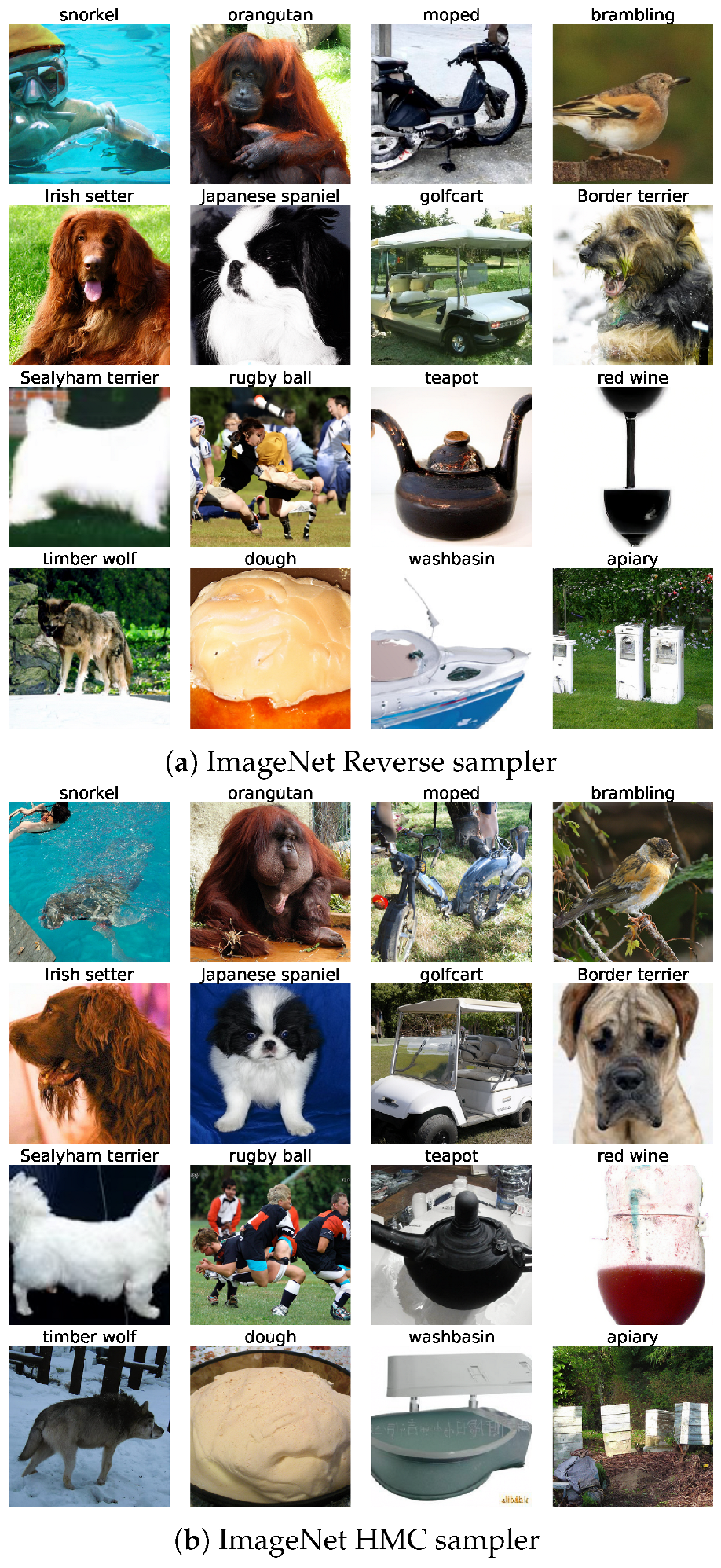
ImageNet: For ImageNet, training diffusion models from scratch requires substantial computational resources, so we relied on widely used pre-trained models. Score-based models are publicly available through the OpenAI GitHub repository (
https://github.com/openai/guided-diffusion, accessed on 4 January 2025), as provided by Dhariwal and Nichol [
10]. However, to our knowledge, there are currently no equivalent publicly available, pre-trained energy-parameterized models at this scale. This limitation highlights the practical value of our approach: by operating directly on pre-trained score models, our method enables MCMC-based refinement even in large-scale settings where explicit energy parameterizations are not readily available. Given the high computational demands of large-scale diffusion models, we focused solely on evaluating HMC and compared it to the reverse process. The HMC sampler adds
MCMC steps per diffusion step
t, with each step consisting of three leapfrog steps, following the setup of the guided diffusion experiment in Du et al. [
18]. For the trapezoidal rule, we used the curve-based integration from Algorithm 3 with
. The step length parameterization and tuning follow the same procedure as in CIFAR-100.
The results can be seen in
Table 4. Accuracy metrics are computed using a pre-trained RegNetX-8.0GF [
40] classifier. The reverse process and HMC perform very similarly in average accuracy, but our method shows a slight improvement in top 5 average accuracy. HMC obtains a significantly better FID score.
4.4. Image Tapestry
We conduct a final, image tapestry experiment, similar to [
18] and based on their code (
https://github.com/yilundu/reduce_reuse_recycle, accessed on 4 January 2025), with only minor modifications to incorporate our MH-like correction. The goal is to generate a coherent image composed of spatially localized content, each region conditioned on different prompts. This task involves both classifier-free guidance and model composition—specifically the combination of multiple overlapping text-to-image diffusion models, each responsible for a portion of the scene.
We use a pre-trained DeepFloyd-IF model (
https://huggingface.co/DeepFloyd/IF-I-XL-v1.0, accessed on 4 January 2025) as the base diffusion model. To refine the generated samples, we apply Langevin dynamics with our MH-like correction. For each diffusion step (
), we include 15 additional Langevin steps. The pseudo-energy difference is approximated via line integration using three additional evaluation points per step. We set the classifier-free guidance scale to
.
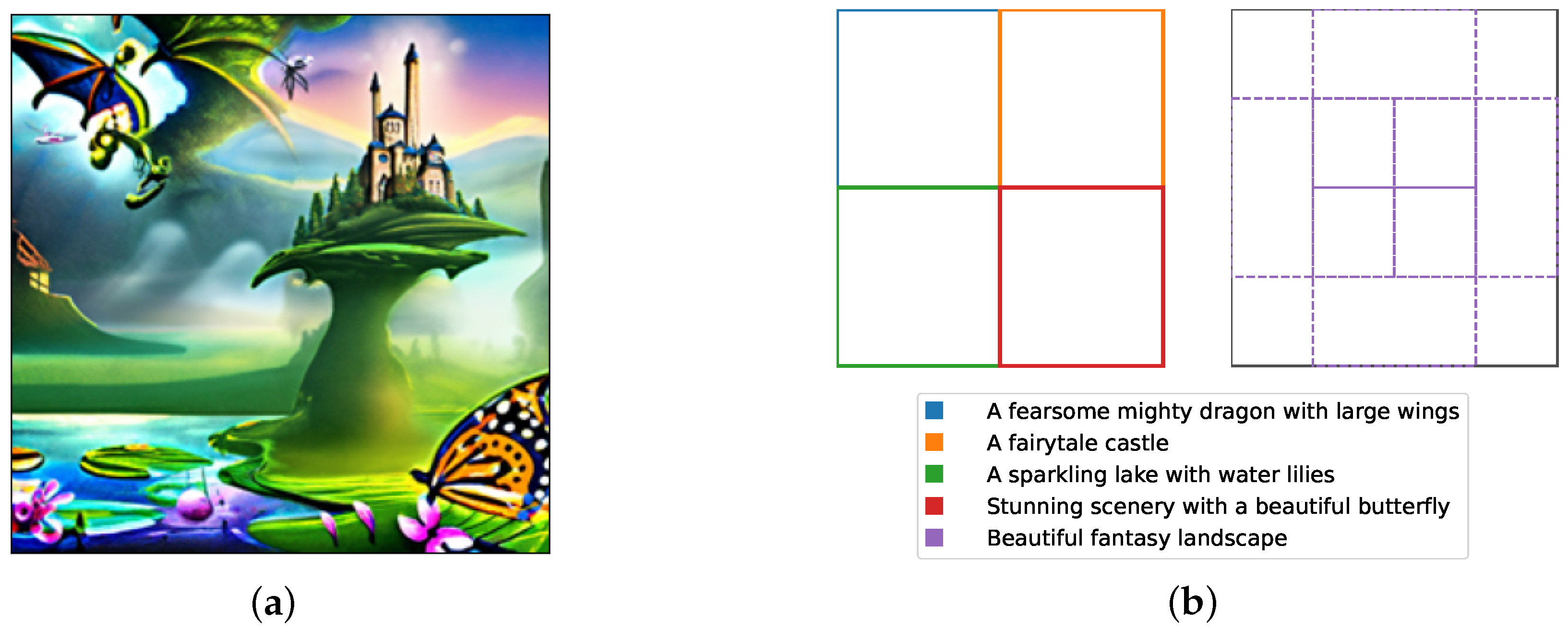
The resulting image is presented in
Figure 2a, which showcases the generated tapestry with different regions displaying distinct visual content.
Figure 2b provides a schematic overview of the used prompts and their spatial layout. In total, nine content regions are specified: four located in the corners of the image, each with unique prompts, and five overlapping in the center, all guided by the same prompt to create a unified visual theme.




 ,
,