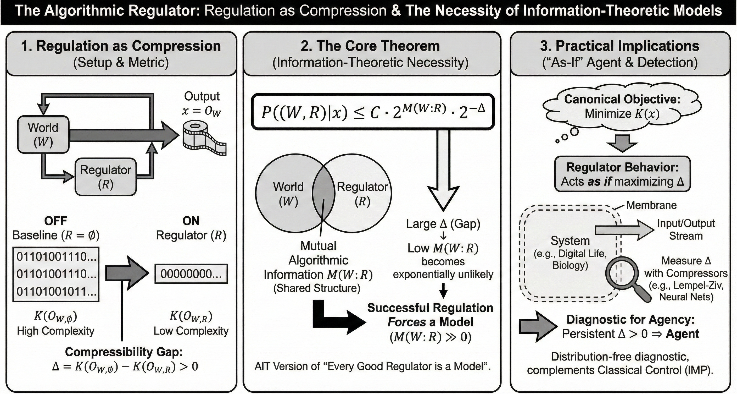
The Algorithmic Regulator

Abstract

The regulator theorem states that, under certain conditions, any optimal controller must embody a model of the system it regulates, grounding the idea that controllers embed, explicitly or implicitly, internal models of the controlled. This principle underpins neuroscience and predictive brain theories like the Free-Energy Principle or Kolmogorov/Algorithmic Agent theory. However, the theorem is only proven in limited settings. Here, we treat the deterministic, closed, coupled world-regulator system (W,R) as a single self-delimiting program p via a constant-size wrapper that produces the world output string x fed to the regulator. We analyze regulation from the viewpoint of the algorithmic complexity of the output, $K\left(x\right)$ (regulation as compression). We define R to be a good algorithmic regulator if it reduces the algorithmic complexity of the readout relative to a null (unregulated) baseline ⌀, i.e., $\Delta =K\left(O_{W,⌀}\right)-K\left(O_{W,R}\right)>0.$ We then prove that the larger $\Delta$ is, the more world-regulator pairs with high mutual algorithmic information are favored. More precisely, a complexity gap $\Delta >0$ yields $Pr((W,R)\mid x)\le C 2^{M(W:R)}{2}^{-\Delta }$, making low $M(W:R)$ exponentially unlikely as $\Delta$ grows. This is an AIT version of the idea that “the regulator contains a model of the world.” The framework is distribution-free, applies to individual sequences, and complements the Internal Model Principle. Beyond this necessity claim, the same coding-theorem calculus singles out a canonical scalar objective and implicates a planner. On the realized episode, a regulator behaves as if it minimized the conditional description length of the readout.

1. Introduction

In the Kolmogorov Theory (KT) of consciousness, an algorithmic agent is a system that maintains (tele)homeostasis (persistence of self or kind) by learning and running succinct generative models of its world coupled to an objective function and a action planner [1,2,3]. Closely related, Active Inference (AIF) models biological agents as minimizing variational free energy under a generative model [4,5]. These frameworks suggest that “agents with world-modeling engines, objective functions, and planners” are natural minimal models of homeostasis (goal-conditioned setpoint control). But for the kinds of homeostatic systems we actually encounter in nature (cells, organisms, engineered servos), how can we tell—operationally—whether they are algorithmic agents in this sense?

Our results are explicitly distribution-free: we do not assume probability densities, and the relevant “model content” can be inferred from a single realized world–regulator instance via algorithmic mutual information. Closest in spirit are algorithmic statistics and MDL (two-part codes/individual-object sufficient statistics), which formalize “model-from-one-object” without an ensemble [6,7,8,9]. In control, “single-trajectory” data-driven methods can identify LTI dynamics from one sufficiently rich trajectory, but only under strong structural assumptions (e.g., LTI, controllability, persistency of excitation) [10]. To our knowledge, there is no analogous distribution-free result that derives a general necessity claim of internal-model content for arbitrary regulators from single-episode data without such structural assumptions; highlighting this gap makes the present AIT results all the more informative.

The classical cybernetics statement that “every good regulator of a system must be a model of that system” originates with Conant and Ashby’s 1970 paper (the Good Regulator Theorem, GRT) [11]. While influential, the GRT has been criticized for the looseness of its definitions of “model” and “goodness”, and for a proof that does not clearly deliver the headline claim [12]. In modern control theory, the rigorous statement that fills a similar conceptual niche is the Internal Model Principle (IMP): under appropriate hypotheses, perfect regulation or disturbance rejection for a given signal class requires that the controller embed a dynamical copy of the signal generator [13,14,15]. The IMP is precise (and falsifiable) within its scope, and is now a standard backbone for robust control; see [16] for a contemporary review across control, bioengineering, and neuroscience. However, the classical IMP is a linear result: for finite-dimensional LTI plants ( linear, time-invariant meaning the system matrices do not change with time) and exogenous signals generated by a finite-dimensional LTI exosystem, robust asymptotic tracking/disturbance rejection requires that the controller embed a copy of the exosystem dynamics [14]. For nonlinear systems, the appropriate generalization is the nonlinear output-regulation framework: if the regulator equations admit smooth solutions and the plant’s zero dynamics on the regulated manifold are (locally) stable, together with suitable immersion/detectability assumptions, then one can construct dynamic output-feedback regulators that embed a (possibly adaptive) internal model and achieve local or semiglobal robust regulation [17,18,19]. However, absent these structural hypotheses, a complete nonlinear analogue of the IMP with the same necessity/robustness guarantees as in the LTI case is not generally available.

Table 1. Side-by-side comparison of the classical Good Regulator Theorem (GRT), the Internal Model Principle (IMP), and an Algorithmic-Information-Theoretic Regulator Theorem (ART). Primary sources: Conant & Ashby (1970) [11], Francis & Wonham (1975) [13], Francis & Wonham (1976) [14], Sontag (2003) [15], and Li & Vitányi (2019) [9].

Aspect	GRT (Conant–Ashby, 1970)	IMP (Francis–Wonham, 1975/76; Sontag, 2003)	ART (Algorithmic, This Work)
Setting/Objects	System S, Regulator R, Disturbances/Inputs D, Outcomes Z. Mapping $\psi :(S,R)\mapsto Z$; compare regulators by entropy of Z.	Plant P in feedback with Controller C; exogenous signals from an exosystem E; regulated output y and error $e=r-y$.	World W and Regulator R are deterministic causal prefix programs (3-tape UTM) that interact over interface tapes for horizon N; readout $x=O_{W,R}^{\left(N\right)}$.
Symbols (explicit)	S (system), R (regulator), D (disturbance/input), Z (outcome), $H(·)$ (Shannon entropy).	P (plant), E (exosystem/signal generator), C (controller), y (regulated output), signal class $\mathcal{U}$ (e.g., steps/sinusoids/polynomials).	W (shortest world program), R (shortest regulator program), $x:=O_{W,R}^{\left(N\right)}$ (ON readout), $y:=O_{W,Ø}^{\left(N\right)}$ (OFF readout), $K(·)$ (prefix complexity), $M(·:·)$ (mutual algorithmic information).
Definition of “model”	Deterministic mapping/homomorphism $h:S\to R$ that preserves task-relevant structure so outcomes have low entropy.	Internal model: a dynamical subsystem embedded in C that reproduces E (controller contains a copy of E’s dynamics; in LTI, matching poles such as integrators/resonators).	Algorithmic model (program): R shares computable structure with W—formally $M(W:R)>0$ (equivalently $K(W\mid R)<K\left(W\right)$); no need for a literal dynamical replica.
Notion of “goodness”	“Maximally successful and simple”: minimize $H\left(Z\right)$ and avoid un-necessary regulator randomness/complexity.	Perfect regulation for a specified class $\mathcal{U}$ (exact asymptotic tracking/disturbance rejection, robustness in class).	Compressibility of realized readout: good if $K\left(x\right)$ is small at the chosen N; use contrastive gap $\Delta :=K\left(O_{W,Ø}^{\left(N\right)}\right)-K\left(O_{W,R}^{\left(N\right)}\right)>0$.
Core Theorem Statement	Among regulators that minimize $H\left(Z\right)$ and are simplest, there is a deterministic $h:S\to R$; informally: “every good regulator is (contains) a model of the system.”	Necessity: perfect regulation for class $\mathcal{U}$ requires C to embed a copy of E (an internal model).	Algorithmic necessity: with ON x and OFF complexity $K\left(O_{W,Ø}^{\left(N\right)}\right)=b$, the universal posterior obeys $Pr((W,R)\mid x,E_b^R)\le C 2^{M(W:R)}{2}^{-\Delta }$. Thus sustained $\Delta >0$ makes low $M(W:R)$ exponentially unlikely; on the realized episode, maximizing ON over OFF likelihood is equivalent (up to $O\left(1\right)$) to minimizing $K\left(x\right)$ (i.e., maximizing $\Delta$).
Assumptions	Z is well-defined from $(S,R)$ and disturbances; regulators compared by $H\left(Z\right)$ and simplicity [11].	Typically finite-dimensional LTI; stabilizable/detectable; E autonomous and neutrally stable; exact asymptotic tracking/rejection for $\mathcal{U}$; robustness in a plant neighborhood [13,14,15].	Deterministic closed coupling; fixed universal prefix machine and horizon N; $W,R$ are minimal self-delimiting programs; constant-overhead wrapper for $(W,R,N)\mapsto O_{W,R}^{\left(N\right)}$; diagnostic readout (contrast usable). In practice, estimate $K(·)$ with fixed MDL codelengths.
Restrictions/Limitations	“Model” notion is weak (mapping); success tied to entropy of Z (can reward trivial predictable outcomes); no explicit stability claims.	Sharpest for LTI; nonlinear/output-regulation extensions add local solvability/detectability/zero-dynamics stability; necessity generally local/structural.	Information-theoretic (not structural) necessity; strength depends on diagnostic $\Delta$; $K(·)$ uncomputable (use fixed compressor/MDL); single-episode statements (with probabilistic tilt).
Scope/Use	Conceptual cybernetics link: regulation ⇒ representation (model-building is compulsory).	Design backbone for robust regulation (integral action, embedded oscillators); concrete synthesis constraints.	Distribution-free, single-episode diagnostics; empirical recipe: fix a lossless compressor, quantize readout, compute ON/OFF code lengths, use $\Delta$ as evidence of model content; complements IMP with universal Occam calculus AIT [9].

provides a comparison of the different regulator theorem statements, which can be compared with the one presented here.

In this paper, we recast the modeling requirement in a setting independent of linearity, probability, exact regulation or specific signal classes, by using algorithmic information theory (AIT). We model a world W and a regulator R as deterministic causal Turing machines that interact over interface tapes. We denote the world output by $x=O_W$ (over some temporal horizon of length N). Our main technical claim is that regulation in the algorithmic sense, i.e., simplicity, forces algorithmic dependence between W and R.

1.1. Definition of Model

A model in the present context is a program capable of compressing (or generating) data. Similarly, “the regulator contains a model of the world” is interpreted in an algorithmic-information sense: the regulator R carries nontrivial information about W, quantified by positive mutual algorithmic information $M(W:R)>0$ (up to the standard $O(log)$ slack). Equivalently, knowing R makes the shortest description of W strictly shorter, $K(W\mid R)<K\left(W\right)$. This notion does not require R to embed a dynamical copy of W; rather, it formalizes “model content” as mutual algorithmic information.

We formalize this with the following definition:

Definition 1

(Algorithmic “internal model”). Given a fixed horizon N (implicitly conditioned), we say that R contains an internal model of W in the algorithmic sense if $M(W:R)>0$ (up to $O(log)$), equivalently $K(W\mid R)<K\left(W\right)$. The magnitude of $M(W:R)$ quantifies the amount of computable structure in W that R carries.

Here, “computable structure” means reusable regularities that admit short descriptions (rules, symmetries, constraints, mechanism parameters). Saying that Rshares computable structure with W means that knowing R makes W cheaper to describe: $K(W\mid R)<K\left(W\right)$, i.e., $M(W:R)>0$. This does not require that the regulator embed a dynamical copy of the exosystem (as in classical IMP); it only requires that the regulator carry algorithmic bits informative about the world’s generative mechanism (e.g., algorithmic elements, time constants, setpoints, disturbance classes, invariances).

The definition grounded on mutual algorithmic information M is further motivated by the following: (i) Machine invariance: M is invariant up to $O\left(1\right)$ under changes of universal machine. (ii) Distribution-free: M is defined for individual objects (programs), not probabilistic models. (iii) Operational meaning:  $M(W:R)$ is precisely the codelength reduction in describing W when R is known, aligning with MDL/Occam reasoning via the Coding Theorem [9,20,21].

This is the appropriate lens for our contrastive results, and it complements the Internal Model Principle, where “model” means a dynamical replica of the Exosystem (a part of the World in our framework) under stated structural hypotheses [14,17,18,19]. Conceptually, our AIT result is complementary to the IMP: whereas the IMP states what structural content must be present in a controller to achieve perfect regulation for a given signal class [13,14,15], our results quantify how much algorithmic information the regulator must carry about the world whenever it succeeds in making the measured outcome compressible.

1.2. Regulation as Compression

We score regulation by how compressible a task-weighted error stream is. Let $x_t$ be the weighted error and $x_{1:T}$ the T-sample string. Fix a prefix-free lossless code (e.g., a universal compressor) and define the per-sample codelength $L_T:=\frac{1}{T}{L}_C\left(x_{1:T}\right)$. A regulator R is better on horizon T when it makes $L_T$ smaller than a null baseline ⌀, i.e., when the contrastive gap $\Delta :=L_T(x;⌀)-L_T(x;R)$ is positive. This choice is natural: for stationary ergodic data, normalized universal codelengths converge almost surely (i.e., with probability one) to the Shannon entropy rate $h\left(x\right)$, and (under standard computability assumptions) $K\left(x_{1:T}\right)/T=h\left(x\right)+o\left(1\right)$ almost surely; thus the Kolmogorov-based criterion reduces to the Shannon criterion when those stochastic assumptions hold—while remaining meaningful outside them [9,22,23].

To see the connection between regulation and compression in more detail, let $h_{x_{1:T}}\left(\alpha \right):={min}_{S\ni x_{1:T}, K\left(S\right)\le \alpha }log\left|S\right|$ denote the Kolmogorov structure function [24]. Regulation amounts to moving down this curve: as the regulator invests model bits (larger $\alpha$), more regularity in $x_{1:T}$ is captured and the residual randomness $h_{x_{1:T}}\left(\alpha \right)$ drops, approaching 0 at perfect regulation. The notion of robability emerges along this path. Replacing set-models by probabilistic models $\left\{P_M\right\}$ turns the two-part description into the standard MDL form

$$L(x_{1:T};M)\approx K\left(M\right)-\sum _{t=1}^{T}log{P}_M\left(x_t\right),$$

where the second term is the ideal codelength under $P_M$ (Shannon coding: $-log{P}_M$) [8,9,23]. If the regulator must hedge over multiple models, the mixture/Bayes code with prior $\pi$ uses $\overline{P}\left(x_{1:T}\right)={\sum }_M\pi \left(M\right)P_M\left(x_{1:T}\right)$ and assigns

$$L_{\mathrm{mix}}\left(x_{1:T}\right)=-log\overline{P}\left(x_{1:T}\right)=-log\sum _M\pi \left(M\right)P_M\left(x_{1:T}\right),$$

a valid prefix code whose regret relative to the best single model $M^{\star }$ is bounded by $-log\pi \left(M^{\star }\right)$; with $\pi \left(M\right)\propto 2^{-K\left(M\right)}$ (Solomonoff/Occam), the penalty matches the model description length [7,8,9,20,25]. Thus, probabilistic/Bayesian regulation is the coding-optimal way to descend $h_{x_{1:T}}\left(\alpha \right)$, aligning with the multi-model argument in [26].

Finally, we can treat the regulator input as an error signal quantized at fixed sensor resolution; the per-sample codelength of $x_{1:T}$ under a universal compressor converges to the entropy rate for stationary sources. For Gaussian processes,

$$h\left(x\right)={\displaystyle \frac{1}{4\pi }}{\int }_{-\pi }^{\pi }log\left(2\pi e{S}_{xx}\left(\omega \right)\right)d\omega ,$$

where $S_{xx}$ is the input power spectral density [22,27] of the error signal x, so attenuating in-band sensitivity (reducing $S_{xx}$ where it matters) reduces codelength [27]. In the scalar white-Gaussian case with variance ${\sigma }^2$, $h=\frac{1}{2}log\left(2\pi e{\sigma }^2\right)$, so smaller-amplitude fluctuations (smaller $\sigma$) mean lower entropy and better compressibility. In short, “compressible error” matches the classical view: good regulation removes variability/uncertainty in the task band and accords with the IMP [14,28].

In the next sections, we first provide an overview of the AIT setting and of the results, followed by the analysis of the single episode scenario. The next section provides a formal definition of the algorithmic regulator and the corresponding theorem.

2. Setting

Unless stated otherwise, U is the standard three–tape universal prefix Turing machine: a read-only input tape holding a self-delimiting program p, a work tape (private scratch memory), and a write-only output tape. When we write $U\left(p\right)=x$ we mean that, upon halting, the contents of the output tape equal x; the work tape is never part of the scored output. The domain of halting programs is prefix-free, so Kraft–McMillan applies and the universal a priori semimeasure $m\left(x\right)={\sum }_{U\left(p\right)=x}{2}^{-\left|p\right|}$ is well defined. By the invariance theorem, replacing U by any other universal prefix machine (single- or multi-tape) changes all complexities only by an additive $O\left(1\right)$; all Coding-Theorem statements we use depend only on prefix-freeness and therefore remain valid up to these constants (see, e.g., [9]). Our use of prefix-free (self-delimiting) programs is a standard coding convention in AIT: it ensures that program lengths satisfy Kraft’s inequality and lets the coding theorem link description length and universal probability cleanly. Any finite description can be made self-delimiting with only $O(logn)$ overhead for length n, so this is not a substantive restriction on real systems; it is a technical requirement of the description language (see Appendix A.3) [9].

The (prefix) Kolmogorov complexity of x is the length of its shortest description,

$$K\left(x\right):=min\left\{\right|p|:U(p)=x\}.$$

Intuitively, $K\left(x\right)$ is the best achievable compressed size of x on U. If $K\left(x\right)\ll \left|x\right|$, then x has a short generative regularity; if $K\left(x\right)\approx \left|x\right|$, x is (algorithmically) random. By the invariance theorem, K is machine-independent up to an additive constant $O\left(1\right)$ [9]. A fundamental limitation is that $K(·)$ is not computable: no algorithm can output $K\left(x\right)$ for all x [9,29]. However, algorithms for upper bounds of $K\left(x\right)$ exist, as we discuss below.

Given auxiliary data y on a read-only auxiliary tape, the conditional complexity

$$K(x\mid y):=min\left\{\right|p|:U(p,y)=x\}$$

is the shortest description of x given y. It operationalizes how much new information is needed to reconstruct x once y is known (e.g., “world given regulator,” or “output given model”).

The mutual algorithmic information (up to the usual $O(log)$ slack) is

$$M(x:y):=K\left(x\right)+K\left(y\right)-K(x,y)=K\left(x\right)-K(x\mid y)=K\left(y\right)-K(y\mid x)\pm O(log).$$

$M(x:y)$ measures the algorithmically shared structure between x and y: how many bits we save when describing one with the help of the other. In our setting, “the regulator contains a model of the world” means $M(W:R)>0$ (information-theoretic dependence); this is a necessary information-theoretic analogue of “model” containment that complements—rather than replaces—the classical IMP notion of a dynamical replica.

Intuitively, strings produced by shorter programs are more likely. Solomonoff–Levin’s universal a priori semimeasure $m\left(x\right)$ and the Coding Theorem link probability and description length,

$$-{log}_{2}m\left(x\right)=K\left(x\right)\pm O\left(1\right),$$

(1)

providing a universal Occam calculus over individual strings [9,20,21,25].

In what follows, a finite temporal horizon N is fixed throughout; unless stated otherwise, we implicitly condition on N (e.g., write $K\left(x\right)$ for $K(x\mid N)$). All $O\left(1\right)$ constants depend only on the choice of U (and the fixed constant-overhead wrapper that decodes $(W,R)$ and simulates their coupling to print the readout), never on particular strings; see Appendix A.2.

The Coupled World-Regulator System

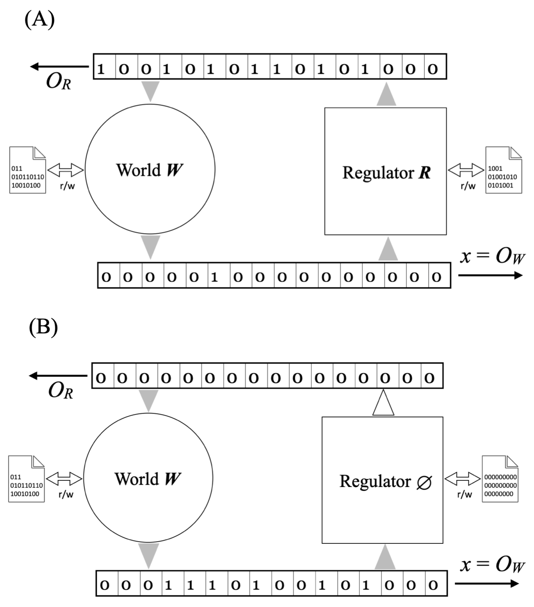
We work with 3-tape Turing machines W and R (see Figure 1 and Appendix A.2). We identify each machine with its minimal self–delimiting program ($\left|W\right|=K\left(W\right)$, $\left|R\right|=K\left(R\right)$) [9]. A horizon $N\in \mathbb{N}$ is fixed and all complexities are conditioned on N unless otherwise stated. W and R interact causally for N steps, producing a deterministic readout $O_{W,R}^{\left(N\right)}\in {\{0,1\}}^N$. The dynamical equations are

$$O_W=W\left(O_R\right),O_R=R\left(O_W\right).$$

(2)

The performance of the regulator is evaluated from the complexity of the output, $K\left(x\right)$. Intuitively, a good regulator produces outputs of lower complexity than the unregulated case. Since $x=O_{W,R}^{\left(N\right)}$ is computable from $(W,R,N)$,

$$K\left(x\right)\le K(W,R)+O\left(1\right)=K\left(W\right)+K\left(R\right)-M(W:R)+O\left(1\right).$$

(3)

To disentangle the role of R from the coarse event “$K\left(O^{\left(N\right)}\right)$ is small,” we fix a null regulator ⌀ (where R’s output is set to zero). We compare the events

$$E_a^R:K\left(O_{W,R}^{\left(N\right)}\right)=a\hspace{1em}\mathrm{vs}\hspace{1em}{E}_b^{⌀}:K\left(O_{W,⌀}^{\left(N\right)}\right)=b,$$

(4)

with $b>a$. Event $E_b^{⌀}$ rules out worlds that produce a simple output without regulation; the intersection $E_a^R\wedge E_b^{⌀}$ isolates R’s contribution.

For notational simplicity, the on–case and off–case readouts are also expressed as

$$x:=O_{W,R}^{\left(N\right)},\hspace{1em}y:=O_{W,⌀}^{\left(N\right)}.$$

For a fixed time horizon, we write $O_W$ for the full output produced by W when coupled to R.

In the next sections, we provide our main results regarding mutual information between the world and regulator, and implications for inferring agent-like behavior in the regulator.

3. Probabilistic Regulator Theorems

3.1. Posterior Form, Given the Observed x

Lemma 1

(Program posterior given x). With prefix prior $P\left(p\right)=2^{-\left|p\right|}$ and deterministic likelihood $P(x\mid p)=\mathbf{1}\left\{U\right(p)=x\}$,

$$P(p\mid x)={\displaystyle \frac{2^{-\left|p\right|}}{m\left(x\right)}}.$$

Consequently, by (5),

$${\displaystyle \frac{1}{c_2}}{2}^{K\left(x\right)-\left|p\right|}\le P(p\mid x)\le {\displaystyle \frac{1}{c_1}}{2}^{K\left(x\right)-\left|p\right|}.$$

Proof. 

For any finite string x,

$$K\left(x\right):=min\left\{\right|p|:U\left(p\right)=x\},\hspace{1em}m\left(x\right):=\sum _{p:U\left(p\right)=x}{2}^{-\left|p\right|}.$$

(recall Equation (1)). The Coding Theorem gives machine-dependent constants $c_1,c_2>0$ with

$$c_1{2}^{-K\left(x\right)}\le m\left(x\right)\le c_2{2}^{-K\left(x\right)}.$$

(5)

Now, briefly, Bayes’ rule yields $Pr\{p\mid x\}=2^{-\left|p\right|}/m\left(x\right)$; apply (5). In more detail, place the prefix prior $P\left(p\right)=2^{-\left|p\right|}$ on programs p and use the deterministic likelihood $P(x\mid p)=\mathbf{1}\left\{U\right(p)=x\}$. Then, the evidence is $P\left(x\right)=m\left(x\right)$ and the posterior is

$$P(p\mid x)={\displaystyle \frac{P(x\mid p)P\left(p\right)}{P\left(x\right)}}=\left\{\begin{array}{cc}{\displaystyle \frac{2^{-\left|p\right|}}{m\left(x\right)},}\hfill & U\left(p\right)=x,\hfill \\ 0,\hfill & \mathrm{otherwise}.\hfill \end{array}\right.$$

Then, for any p with $U\left(p\right)=x$,

$${\displaystyle \frac{1}{c_2}}{2}^{K\left(x\right)-\left|p\right|}\le P(p\mid x)={\displaystyle \frac{2^{-\left|p\right|}}{m\left(x\right)}}\le {\displaystyle \frac{1}{c_1}}{2}^{K\left(x\right)-\left|p\right|}.$$

The relation between $K\left(x\right)$ and $m\left(x\right)$ holds only up to an additive $O\left(1\right)$ term in K, which becomes a multiplicative constant on $m\left(x\right)$. This $O\left(1\right)$ ambiguity is unavoidable and depends on the choice of universal prefix machine U; $c_1,c_2$ absorb exactly this machine-dependent slack. □

Now, in our setting the world W and regulator R are programs that interact for N steps, producing the on-case readout $x:=O_{W,R}^{\left(N\right)}$. A fixed, constant-overhead wrapper decodes a shortest description of $(W,R)$ and simulates the coupling to print x (decode + simulate); if $p_{W,R}$ denotes this canonical code, then

$$|p_{W,R}|=K(W,R)+O\left(1\right),\hspace{1em}P\left((W,R)\mid x\right)\in \left[\frac{1}{{\tilde{c}}_2},\frac{1}{{\tilde{c}}_1}\right]·2^{K\left(x\right)-K(W,R)},$$

(6)

for constants ${\tilde{c}}_i:=2^{O\left(1\right)}{c}_i$.

Now we can use the definition of mutual algorithmic information (up to the usual $O(log)$ slack) to write

$$M(W:R)=K\left(W\right)+K\left(R\right)-K(W,R)$$

and derive our first result:

Theorem 1.

$$P\left((W,R)\mid x\right)\in \left[\frac{1}{{\tilde{c}}_2},\frac{1}{{\tilde{c}}_1}\right]·2^{K\left(x\right)-K\left(W\right)-K\left(R\right)+M(W:R)}<{\displaystyle \frac{1}{\tilde{c}}}{2}^{M(W:R)}$$

(7)

3.2. The Good Algorithmic Regulator and Posterior with Contrast

For our second result, we first define the Good Algorithmic Regulator (GAR).

Definition 2

(Good Algorithmic Regulator, contrastive). Given the on/off complexities and gap

$$a:=K\left(O_{W,R}^{\left(N\right)}\right),\hspace{1em}b:=K\left(O_{W,⌀}^{\left(N\right)}\right),\hspace{1em}\Delta :=b-a.$$

we say that R is a good algorithmic regulator of gap $\Delta$ for W at horizon N if $\Delta >0$.

Lemma 2

(OFF run lower-bounds the world). There exists $c_0=O\left(1\right)$ such that

$$K\left(O_{W,⌀}^{\left(N\right)}\right)\le K\left(W\right)+c_0\hspace{1em}\Rightarrow \hspace{1em}K\left(W\right)\ge b-c_0.$$

Proof. 

Given $(W,⌀,N)$, the wrapper simulates the OFF dynamics and prints $O_{W,⌀}^{\left(N\right)}$ with $O\left(1\right)$ overhead. □

With this definition we can now state and prove our main theorem.

Theorem 2

(Probabilistic regulator theorem). Let $O_{W,R}^{\left(N\right)}$ and ${\mathsf{E}}_b^R$ be observed and let $\Delta :=K\left(O_{W,⌀}^{\left(N\right)}\right)-K\left(O_{W,R}^{\left(N\right)}\right)$. Then, there exists $C>0$ such that

$$P\left((W,R)\mid O_{W,R}^{\left(N\right)},{\mathsf{E}}_b^R\right)\le C·2^{M(W:R)}{2}^{-\Delta }.$$

Equivalently, every bit by which $M(W:R)$ falls short of Δ costs a factor $\approx 2^{-1}$ in posterior support.

Proof. 

(i) Posterior via wrapper. From Equation (6), ${log}_{2}P((W,R)\mid x)\le K\left(x\right)-K(W,R)+O\left(1\right)=a-K(W,R)+O\left(1\right).$

(ii) Decompose $K(W,R)$. We use the exact mutual information $M(W:R):=K\left(W\right)+K\left(R\right)-K(W,R)$, $K(W,R)=K\left(W\right)+K\left(R\right)-M(W:R),$ hence

$$K\left(x\right)-K(W,R)=a-K\left(W\right)-K\left(R\right)+M(W:R).$$

(iii) Insert OFF bound (where b enters). By Lemma 2, $K\left(W\right)\ge b-c_0$, so

$$K\left(x\right)-K(W,R)\le M(W:R)-(b-a)-K\left(R\right)+c_0=M(W:R)-\Delta -K\left(R\right)+c_0.$$

(iv) Exponentiate and absorb constants. Exponentiating and using $2^{-K\left(R\right)}\le 1$ gives $P((W,R)\mid x,{\mathsf{E}}_b^R)\le C 2^{M(W:R)}{2}^{-\Delta }$ for a constant C absorbing $2^{c_0}$ and the wrapper Coding-Theorem constants. □

• Clarifications:

(i) Where does b appear? Only via Lemma 2, which says the OFF run lower-bounds $K\left(W\right)$. We never need to compute b explicitly. (ii) Why can we drop $2^{-K\left(R\right)}$? A slightly sharper bound is $P((W,R)\mid x,{\mathsf{E}}_b^R)\le C 2^{M(W:R)}{2}^{-\Delta }{2}^{-K\left(R\right)}$. Since $K\left(R\right)\ge 0$, dropping $2^{-K\left(R\right)}\le 1$ keeps the focus on the two interpretable scalars M and $\Delta$ without changing the exponential scaling. (iii) Architecture-agnostic. The proof only uses the computable wrapper $(W,R,N)\mapsto x$. Whether R is open- or closed-loop does not affect the posterior algebra. (iv) The posterior on the left of Theorem 2 is conditioned on the on-case observation x only. The off-case run is used solely to supply a numeric lower bound $b:=K\left(O_{W,⌀}^{\left(N\right)}\right)$, which implies $K\left(W\right)\ge b-O\left(1\right)$ by simulation. Formally, we phrase the result as a bound on $Pr((W,R)\mid x,{\mathsf{E}}_b^R)$, where ${\mathsf{E}}_b^R$ is the side-event “$K\left(O_{W,⌀}^{\left(N\right)}\right)=b$”.

As a consequence of Theorem 2, one can bound individual posterior masses by $O\left(2^{K\left(x\right)-K(W,R)}\right)$. This implies an exponential tail: $PrM(W:R)\le \Delta -k=O\left(2^{-k}\right)$. In other words, $M(W:R)$ is concentrated within $O\left(1\right)$ of its maximum $\Delta$. I.e., there exists $C^{\prime }>0$ (machine/wrapper dependent only) such that for all integers $k\ge 0$,

$$Pr\left\{M(W:R)\le \Delta -k | x,{\mathsf{E}}_b^R\right\}\le C^{\prime }{2}^{-k}.$$

How to read (and use) Theorem 2:

• What we measure: compute the on/off complexities $a=K\left(O_{W,R}^{\left(N\right)}\right)$ and $b=K\left(O_{W,⌀}^{\left(N\right)}\right)$ (in practice: fixed MDL code lengths); their difference $\Delta =b-a$ is the compressibility advantage.
• What the bound says: for any explanation $(W,R)$ of the observed x, the universal posterior weight is penalized as $2^{-\Delta }$ unless the pair shares structure: larger $M(W:R)$ compensates the penalty.
• Practical rule of thumb: sustained large $\Delta$ across tasks makes low $M(W:R)$ exponentially unlikely. If off-case b is already small, $\Delta$ will be small—choose a diagnostic readout so the null is not trivially simple.

3.3. Inferring the Objective Function and Planner (As-If Agent)

We next provide a simple theorem regarding the role of complexity as an objective function.

Theorem 3

(On/Off evidence equals unconditioned complexity gap). Under the universal a priori semimeasure,

$${log}_2{\displaystyle \frac{m\left(O_{W,R}^{\left(N\right)}\right)}{m\left(O_{W,⌀}^{\left(N\right)}\right)}}=K\left(O_{W,⌀}^{\left(N\right)}\right)-K\left(O_{W,R}^{\left(N\right)}\right)\pm O\left(1\right).$$

(8)

Equivalently, writing the on/off gap as $\Delta :=K\left(O_{W,⌀}^{\left(N\right)}\right)-K\left(O_{W,R}^{\left(N\right)}\right),$ we have $m\left(O_{W,R}^{\left(N\right)}\right)/m\left(O_{W,⌀}^{\left(N\right)}\right)=\mathrm{\Theta }\left(2^{\Delta }\right).$ Hence, on the realized pair $(O_{W,R}^{\left(N\right)},O_{W,⌀}^{\left(N\right)})$, maximizing the likelihood of “ON over OFF” is equivalent (up to a constant factor) to minimizing $K\left(O_{W,R}^{\left(N\right)}\right)$ or, equivalently, maximizing the gap Δ.

Proof. 

By the Coding Theorem there exist machine-dependent constants $c_1,c_2>0$ such that $c_1{2}^{-K\left(z\right)}\le m\left(z\right)\le c_2{2}^{-K\left(z\right)}$ for any string z. Apply this to x and $O_{W,⌀}^{\left(N\right)}$, take base-2 logs, and subtract:

$$-{log}_{2}m\left(O_{W,R}^{\left(N\right)}\right)=K\left(O_{W,R}^{\left(N\right)}\right)\pm O\left(1\right),\hspace{1em}-{log}_{2}m\left(O_{W,⌀}^{\left(N\right)}\right)=K\left(O_{W,⌀}^{\left(N\right)}\right)\pm O\left(1\right),$$

so ${log}_2\frac{m\left(O_{W,R}^{\left(N\right)}\right)}{m\left(O_{W,⌀}^{\left(N\right)}\right)}=K\left(y\right)-K\left(O_{W,R}^{\left(N\right)}\right)\pm O\left(1\right).$ □

This statement compares two different strings (the realized ON and OFF outputs) and aligns with the contrastive quantities used elsewhere. The log universal Bayes factor for “ON vs. OFF” is seen to equal the complexity gap $\Delta \pm O\left(1\right).$ Thus, on each episode, a regulator behaves as if it were maximizing the scalar $\Delta ,$ equivalently minimizing $K\left(O_{W,R}^{\left(N\right)}\right)$.

Thus, given a regulator R that persistently reduces the readout’s complexity relative to a null baseline ⌀ (the GAR setting of Definition 2), we can justify—on purely observational grounds—that R behaves as if it were minimizing a scalar objective. The objective should be canonical (not post hoc) and usable across episodes/tasks.

4. Discussion

Classical control theory—especially in the LTI case—provides powerful constructive synthesis methods yielding transparent regulator architectures under explicit model classes. Our results are different in scope: they give a distribution-free, single-instance necessity/diagnostic statement. If regulation induces a nontrivial contrastive compressibility gap, then the regulator R must carry algorithmic information about the world W.

However, this theoretical necessity does not by itself provide a controller design algorithm, and its practical application relies on computable surrogates for Kolmogorov complexity, such as Lempel-Ziv compression [22] or neural autoencoders [30,31]. Furthermore, to detect agency in a biological or social system, or in digital life systems—such as Conway’s Game of Life [32] or continuous cellular automata like Lenia [33,34]—one must first tentatively define a “membrane” (Markov blanket [5,35,36]) that separates the putative agent R from its environment W. By inspecting the input-output stream across various candidate boundaries, we can identify agents as those subsystems that maximize the compressibility gap $\Delta$. In this sense, while probabilistic and model-class-based approaches remain indispensable for constructive designs and performance guarantees, our AIT framework acts as an “outer layer” diagnostic that characterizes when “having a model” (in the information-theoretic sense) is unavoidable.

We summarize now our results:

• First regulator result: posterior form, given the observed x (Theorem 1).

By Solomonoff induction and the Coding Theorem [20,21,25,37,38], we showed that

$$Pr\left((W,R)\mid x\right)={\displaystyle \frac{2^{-K(W,R)+O\left(1\right)}}{m\left(x\right)}}\sim 2^{K\left(x\right)-K(W,R)}<{\displaystyle \frac{1}{\tilde{c}}}{2}^{M(W:R)}$$

(9)

Thus shorter joint generators are exponentially preferred; every extra bit in $K(W,R)$ halves the posterior weight. Decomposing

$$K(W,R)=K\left(W\right)+K\left(R\right)-M(W:R)\pm O(log)$$

(10)

shows that, at fixed marginals $K\left(W\right),K\left(R\right)$, the posterior is exponentially tilted in the algorithmic mutual information $M(W:R)$: each extra bit of $M(W:R)$ multiplies posterior odds by $\approx 2$.

• Second regulator result: posterior with contrast (Theorem 2).

Without contrast, the story is pure Occam: (9) anchors the posterior near $K(W,R)\approx K\left(x\right)$ with a geometric excess-length tail; for fixed $K\left(W\right),K\left(R\right)$, this yields a high-probability lower bound on $M(W:R)$ roughly $K\left(W\right)+K\left(R\right)-K\left(x\right)$. With contrast, if turning the regulator on yields $K\left(O_{W,R}^{\left(N\right)}\right)=a$ while the off case has $K\left(O_{W,⌀}^{\left(N\right)}\right)=b$ with $b>a$, then any explaining $(W,R)$ obeys

$$Pr((W,R)\mid x)\le C{2}^{M(W:R)}{2}^{-\Delta },$$

so low mutual information is exponentially disfavored as the gap $\Delta =b-a$ grows. In both regimes, the operational slogan holds: see a simple string ($K\left(x\right)$ small), suspect a simple generator ($K(W,R)$ small), and at fixed marginals, this means suspect larger $M(W:R)$.

The intuition behind these results is that seeing a simple string suggests its generation by a simple program. Formally, for the coupled hypothesis $P=(W,R)$ (wrapped as a single self-delimiting program), observing $x=O_W^{\left(N\right)}$ yields the Solomonoff posterior $Pr(P\mid x)\sim 2^{K\left(x\right)-K\left(P\right)},$ by the Coding Theorem [20,21,25,37,38]. Every extra bit of joint description $K\left(P\right)=K(W,R)$ halves posterior weight. This is the quantitative Occam tilt that operationalizes the slogan above.

The posterior mass of joint programs longer than $K\left(x\right)+k$ decays geometrically:

$$Pr\{K(W,R)\ge K\left(x\right)+k\mid x\}\le 2C 2^{-k}.$$

Hence, the typical joint length is near $K\left(x\right)$. If $K\left(W\right)$ and $K\left(R\right)$ are externally constrained (e.g., by design or prior knowledge), this tail translates directly into a lower posterior bound on $M(W:R)$ of the form $M(W:R)\gtrsim K\left(W\right)+K\left(R\right)-K\left(x\right)-O(log(1/\delta \left)\right)$ with posterior confidence $1-\delta$.

Our results are most informative when the observed readout $O_W^{\left(N\right)}$ is simple. If $K\left(O_W^{\left(N\right)}\right)$ is large, the posterior constraints on joint complexity and on mutual information are inherently weak. From the geometric tail, for any $\delta \in (0,1)$ there exists $k=\lceil {log}_2(2C/\delta )\rceil$ such that, with posterior probability at least $1-\delta$,

$$K(W,R)\le K\left(O_W^{\left(N\right)}\right)+k.$$

At fixed marginals $K\left(W\right)$ and $K\left(R\right)$ this yields

$$M(W:R)\ge K\left(W\right)+K\left(R\right)-K\left(O_W^{\left(N\right)}\right)-k-O(log)\hspace{1em}\mathrm{with}\mathrm{probability}\ge 1-\delta .$$

Hence, if $K\left(O_W^{\left(N\right)}\right)$ is large (comparable to $K\left(W\right)+K\left(R\right)$), the lower bound on $M(W:R)$ may be trivial (near 0 up to logs). Intuitively, a complex output does not force shared structure. It is compatible with a complex joint generator even when W and R share little algorithmic information.

On the other hand, the strength of the conclusion depends on the gap $\Delta =b-a$:

$$Pr\left((W,R)\mid O_W^{\left(N\right)},{\mathsf{E}}_b^R\right)\le C 2^{M(W:R)}{2}^{-\Delta },\hspace{1em}Pr\left\{M(W:R)\le \Delta -k|O_W^{\left(N\right)},{\mathsf{E}}_b^R\right\}\le C^{\prime }{2}^{-k}.$$

Thus even if $a=K\left(O_{W,R}^{\left(N\right)}\right)$ is not very small, a large off/on gap still enforces a large posterior $M(W:R)$. In other words, contrast rescues identifiability of shared structure: the evidence scales exponentially in $\Delta$.

In the same universal calculus, regulation carries a canonical scalar interpretation: runtime behavior is as if minimizing $K\left(O_W^{\left(N\right)}\right)$ (i.e., maximizing the on/off gap $\Delta$), and design-time comparison across explanations favors larger $M(W:R)-\Delta$ via the GAR posterior tilt. This supplies an MDL/Occam objective grounded in the coding theorem (not an ad hoc utility) and complements the IMP’s structural requirements.

We note that a low $K\left(O_W^{\left(N\right)}\right)$ alone does not prove high $M(W:R)$; it concentrates posterior mass on short joint generators P. High $M(W:R)$ follows (i) when $K\left(W\right)$ and $K\left(R\right)$ are fixed/known, or (ii) when contrast pins $K\left(W\right)$ high via the off case. Without such constraints, short P could also arise from individually simple W and R.

• Third regulator result: as-if Objective-function minimization (Theorem 3).

On the realized $O_W^{\left(N\right)}$, the conditional Coding Theorem gives ${log}_2\left(m\left(O_W^{\left(N\right)}\right)/m\left(O_{W,⌀}^{\left(N\right)}\right)\right)=K\left(O_{W,⌀}^{\left(N\right)}\right)-K\left(O_W^{\left(N\right)}\right)$. Thus, the runtime scalar to minimize is $K\left(O_W^{\left(N\right)}\right)$. Together with the above, this implies that the regulator is acting (as-if) like an algorithmic agent (with a model of the world, objective function and planner).

Theorem 3 is a representation statement—not a mechanism: R need not compute K, but persistent large $\Delta$ is exactly what maximizes universal evidence for “ON”, and it simultaneously makes low $M(W:R)$ exponentially unlikely. For a mechanistic objective beyond the Minimum Description Length (MDL) evidence, three constructive routes are standard and complementary. First, in Linear Time-Invariant (LTI) plants the Internal Model Principle makes a structural claim—perfect robust regulation for a specified signal class requires embedding a dynamical copy of the exosystem in the controller—and optimal stabilizing designs arise from explicit quadratic/convex costs (e.g., the Linear Quadratic Regulator, LQR); in the nonlinear case, output-regulation theory yields constructive regulators under solvable regulator equations together with immersion/detectability and (local) zero-dynamics stability [13,14,15,17,18,19,39]. Second, in inverse optimal control and inverse reinforcement learning (IRL), trajectories that satisfy Karush–Kuhn–Tucker (KKT) regularity allow identification of a cost J (up to equivalences) whose minimizers reproduce the behavior; in discrete settings, IRL recovers reward functions consistent with observed policies [40,41,42]. Third, in revealed-preference analysis, if cross-episode choices satisfy the Generalized Axiom of Revealed Preference (GARP), Afriat and Varian guarantee the existence of a strictly increasing, concave utility that rationalizes the data, while Debreu’s representation and the Savage/Karni–Schmeidler frameworks provide (state-dependent) expected-utility forms under their axioms [43,44,45,46,47].

• Planner/policy representation (as-if agent).

Any deterministic causal regulator R induces a computable policy ${\pi }_R:{\mathcal{H}}_t\to \mathcal{A}$ mapping the coupled history $h_t$ (past interface I/O up to time t) to the next actuator symbol. This is simply the operational semantics of R viewed as a function of histories.

The coding-theorem Bayes-factor identity (Theorem 3) supplies a canonical scalar such that, on the realized episode, the sequence of actions produced by ${\pi }_R$ is as if chosen to maximize J subject to the world dynamics. Together with the algorithmic “internal model” conclusion $M(W:R)>0$ (i.e., $K(W\mid R)<K\left(W\right)$), this yields the standard agent triad:

$$\left(\mathrm{model}\right)M(W:R)>0,\hspace{1em}\left(\mathrm{objective}\right)J\left(x\right)=K\left(y\right)-K\left(x\right),\hspace{1em}(\mathrm{policy}/\mathrm{planner}){\pi }_R.$$

Interpretation. This is a representation statement, not a claim that R explicitly solves an optimization problem or contains a modular planner. The existence of ${\pi }_R$ is tautological for any deterministic R; the “as-if” objective follows from the universal evidence identity above. Across tasks/episodes, if the induced choices satisfy standard consistency axioms (e.g., GARP), classical revealed-preference theorems guarantee the existence of a (monotone, concave) utility that rationalizes the behavior [43,44]; and in dynamical settings, inverse optimal control/inverse RL constructs a cost for which the observed policy is (near-)optimal [40,41]. Thus, given (i) algorithmic model content $M(W:R)>0$ and (ii) the canonical scalar J from the coding-theorem calculus, interpreting the regulator as carrying a policy/planner is both natural and technically justified.

4.1. Why AIT Is Needed

Our results are single-episode and distribution-free: they make statements about an individual realized readout x and about the pair $(W,R)$ as concrete programs, without positing a stochastic source. Classical (Shannon) information theory quantifies expected code lengths and mutual information with respect to a specified probability law; entropy $H\left(X\right)$ and mutual information $I(X;Y)$ are undefined without a distribution, and asymptotic statements (AEP/typical sets) further require ergodicity/mixing assumptions [23]. In our setting, there is no given probabilistic model over worlds, regulators, or outputs—indeed, the point is to infer model content from a single realized x.

AIT supplies exactly the missing calculus. First, it provides a canonical, machine-invariant complexity for individual strings, $K\left(x\right)$, and a universal a priori semi measure $m\left(x\right)$ (Solomonoff– Levin), connected by the Coding Theorem: $-logm\left(x\right)=K\left(x\right)\pm O\left(1\right)$ [20,21,25]. This yields a universal Occam posterior over programs, $Pr\left(p\mid x\right)\asymp 2^{K\left(x\right)-\left|p\right|},$ from which (i) the geometric excess-length tail and (ii) our contrastive tilt bounds follow. No analogue exists in Shannon’s framework without positing an external prior over programs; there is no “canonical” $Pr\left(p\right)$ or $Pr\left(x\right)$ in Shannon theory.

Second, AIT lets us formalize “the regulator contains a model of the world” as algorithmic dependence, i.e., positive mutual algorithmic information $M(W:R)>0$ (equivalently $K(W\mid R)<K\left(W\right)$), a notion defined for individual objects and invariant up to $O\left(1\right)$ [9]. By contrast, Shannon’s $I(W;R)$ requires a joint distribution over $(W,R)$, which is neither given nor natural here.

Third, our key inequalities explicitly use $m(·)$ and prefix complexity: the posterior tilt $2^{K\left(x\right)-K(W,R)}$, the OFF-run lower bound on $K\left(W\right)$ by simulation, and the contrastive penalty $2^{-\Delta }$ all rely on the Coding Theorem and Kraft–McMillan properties of prefix programs—again, objects absent from Shannon’s ensemble-level calculus.

Finally, while one can approximate $K(·)$ with MDL/codelengths in practice, MDL’s justification itself rests on the AIT view that shorter descriptions are better and on the coding-theorem linkage between description length and (universal) probability [8]. In short: AIT provides the universal prior (m), object-level complexities (K), and mutual algorithmic information (M) needed to turn the informal slogan “see a simple string, suspect a simple generator” into posterior and contrastive theorems—none of which can be stated in Shannon’s framework without ad hoc model classes and priors.

4.1.1. Relation to the Internal Model Principle (IMP)

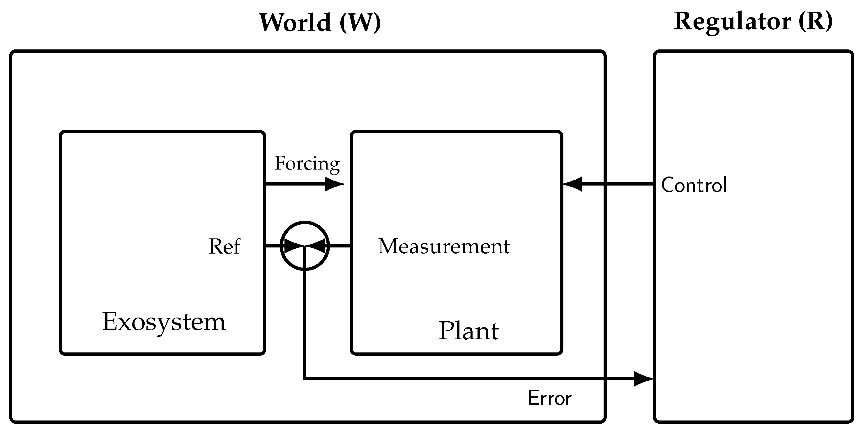
In the IMP, the closed loop is $(E,C,P)$: an autonomous exosystem E (no inputs and no explicit time dependence, e.g., $\dot{w}=Sw$), a controller C (the regulator), and a plant P. The regulated error is $e=r-y$, where the reference r and disturbances are generated by E and y is measured from P [13,14]. In our notation, we group the World as $W=(E,P)$ and take the Regulator as $R\equiv C$ (see Figure 2 and

Table 2. Mapping the IMP triple $(E,C,P)$ and the AIT $(W,R)$ view to a simple thermostat. IMP emphasizes an internal model of the exosystem E for exact regulation over a signal class; AIT treats $W=(P,E)$ jointly and assesses regulation by a compressibility advantage $\Delta$.

Role	IMP Language	AIT Language (This Work)	Thermostat Instantiation
Exogenous generator	Exosystem E: autonomous generator of references/disturbances (no feedback from C); exact regulation is defined w.r.t. a signal class $\mathcal{U}$.	Fold into the World W; no architectural split is required (but may still conceptually identify this subpart).	Reference$r\left(t\right)$: setpoint schedule (often clock-driven). Disturbances: outdoor temperature, solar load, occupancy heat gains.
Plant	Plant P: room thermal dynamics + actuator/sensor; used for stabilization/shaping.	Also inside World W.	R–C (thermal) model, heater actuation, heat losses, sensor dynamics/delay.
Controller/ Regulator	Controller C (the regulator in IMP).	Regulator R.	Thermostat logic: bang-bang with hysteresis, PI/TPI, or scheduled control.
Measured output	y.	World readout x extracted from the transcript (often $x=y$ or the error string $e_{1:T}$).	Indoor temperature $T_{\mathrm{in}}$ (or a weighted error signal).
Error/ objective	$e=r-y$; IMP concerns asymptotic $e\to 0$ for all $r,d$ in the class $\mathcal{U}$ (internal model must match E).	Score regulation by compressibility of the chosen readout x with R ON vs. an OFF baseline ($R=⌀$). Define the gap $\Delta =K\left(x_{\mathrm{off}}\right)-K\left(x_{\mathrm{on}}\right)$ (practically, use a fixed MDL code $L_C$ in place of K).	Good thermostat ⇒ $x_{\mathrm{on}}$ (e.g., temperature or error) stays near a regular deadband pattern ⇒ shorter code than the null/open-loop case (heater OFF or fixed duty).

for the comparison of the two frameworks in the case of a thermostat).

The assumptions in the IMP theorems are: (i) Classical necessity is sharpest for finite-dimensional LTI plants (linear, time-invariant) with exogenous signals generated by a finite-dimensional, neutrally stable LTI E; stabilizability/detectability and robustness (one fixed C works for a plant neighborhood) are standard [13,14]. (ii) The structural conclusion is internal-model necessity: perfect robust regulation for the specified signal class requires that C embed a dynamical copy of E (e.g., integrators for steps, oscillators for sinusoids); in MIMO, a p-copy is needed. (iii) Nonlinear generalizations (output regulation) require solvability of the regulator equations, suitable immersion/detectability, and (local) stability of the zero dynamics; guarantees are typically local/semiglobal, and necessity is not universal [17,18,19]. (iv) Infinite-dimensional/distributed settings and periodic signals may require infinite-dimensional internal models; technicalities arise with unbounded I/O operators [16].

In the AIT formulation (here), we assume: (i) Architecture-agnostic: no required split into E vs. P, and no specified place where R enters the causal path; we only assume a computable wrapper mapping $(W,R,N)\mapsto O_W$ for a fixed horizon N. (ii) Deterministic, closed coupling of world and regulator (no stochastic noise sources into W); statements are distribution-free and about the realized sequence. (iii) “Model” means algorithmic dependence: $M(W:R)>0$ (equivalently $K\left(W\right|R)<K(W)$), not a literal dynamical replica. (iv) The main necessity is probabilistic: a positive on/off complexity gap $\Delta =K\left(O_{W,Ø}\right)-K\left(O_{W,R}\right)$ exponentially tilts the universal posterior against explanations with small $M(W:R)$; no linearity, smoothness, or regulator-equation conditions are imposed. See Section 2, Section 3, Section 4 and Section 5 and Appendix A of this work.

IMP yields a structural necessity (internal model in C of E) under explicit dynamical hypotheses; the AIT formulation yields an information-theoretic necessity (positive $M(W:R)$ favored by the data) without assuming linearity, an $E/P$ split, or a particular causal insertion point for R. The two are complementary: IMP is the backbone for constructive regulation in structured classes; the AIT view covers unstructured architectures and single episodes with a universal Occam calculus [13,14,15,16,17,18].

• The home thermostat.

As an example, consider a home thermostat as a regulator/controller. Let P be the living room + heater dynamics (thermal capacitance, heat loss, delays) and E the exogenous processes (setpoint schedule, outdoor weather/solar, occupancy). The Internal Model Principle (IMP) states that exact output regulation for a specified signal class is possible only if the controller embeds a copy of the exosystem E that generates those signals (e.g., an integrator for steps, an oscillator for a fixed sinusoid); plant knowledge is used for stabilization/shaping, but the IMP necessity targets E itself [14,17]. In our AIT view, a regulator R is “good” when it makes the realized readout more compressible than a null baseline; a sustained compressibility gap implies that R shares computable structure with the whole world $W=(P,E)$:

$$M(W:R)=M\left((P,E):R\right)=M(P:R)+M(E:R\mid P)\pm O(log).$$

A simple on/off thermostat with a deadband tuned to the room time constant typically yields a bounded limit cycle (not zero steady-state error); under IMP, it lacks the needed internal model of constants (no embedded integrator), hence it does not achieve exact regulation of the “constant” class [14,28]. Nevertheless, in the AIT sense, it still qualifies as a regulator: its policy encodes a very compressed model spanning P (heating raises T, room inertia) and weak regularities in E (quasi-constant setpoint, slowly varying weather), giving $M(W:R)>0$ [11]. PI/PID or predictive thermostats remedy the IMP shortfall by embedding the appropriate internal model (and often explicit models of P and aspects of E) [28].

The AIT regulator framework (as well as the original GRT) is therefore more general than IMP: the regulator must carry a model of the world $W=E\cup P$, where P is the plant (house/HVAC thermodynamics) and E the exogenous processes (setpoint schedule, weather/solar/occupancy), and IMP is recovered as a special case when the performance target is exact output regulation over a specified signal class. Under IMP, a controller qualifies for exact regulation only if it embeds a dynamical copy of the exosystem that generates the reference/disturbances (e.g., an integrator for steps, oscillators for sinusoids)—no model of P is required beyond stabilizability/detectability [14]; nonlinear output regulation extends this under additional immersion/detectability and regulator-equation solvability assumptions [17].

Our statements are thus complementary and distinct: in AIT, we work in a distribution-free, program-level setting and make no linearity or smoothness assumptions. We remain agnostic about what the regulator needs to model and do not demand exact regulation. We do not assert the existence of a dynamical replica inside R. Instead, we show that sustained contrastive compressibility ($\Delta >0$) tilts the universal posterior toward pairs $(W,R)$ with larger mutual algorithmic information $M(W:R)$, i.e., R carries algorithmic structure about W. Thus, “the regulator contains a model” is made precise as $M(W:R)>0$ (information-theoretic dependence), not as an embedded exosystem. The IMP supplies structural necessity for perfect regulation within specified signal classes; our AIT results supply information-theoretic necessity for observed compressibility advantages, beyond linearity or probabilistic assumptions [15].

4.1.2. Practical Estimation of K and the Gap $\Delta$

Our theorems are stated in terms of prefix Kolmogorov complexity, which is not computable. In practice, one can fix a reference prefix code C and estimate upper bounds,

$$\widehat{a}:=L_C\left(O_{W,R}^{\left(N\right)}\right),\hspace{1em}\widehat{b}:=L_C\left(O_{W,⌀}^{\left(N\right)}\right),\hspace{1em}\widehat{\Delta }=\widehat{b}-\widehat{a},$$

with the same compressor C used across all conditions. Persistent $\widehat{\Delta }>0$ across tasks is cumulative evidence that explanations with low $M(W:R)$ are exponentially unlikely; maximizing $\widehat{\Delta }$ is the natural scalar objective, the regulator appears to optimize on the observed data.

Some standard choices for providing upper bounds to Kolmogorov complexity are Lempel-Ziv compressors (LZ77/LZ78/LZW). LZ-type compressors are universal in a weak sense for stationary ergodic sources and are widely available. Implementations (gzip, lz4, etc.) are practical proxies for $L_C(·)$ [22,48]. If both ON and OFF strings are available and a scale-free sanity check of contrast is needed, we can compute

$$\mathrm{NCD}(x,y):={\displaystyle \frac{C\left(xy\right)-min\left\{C\right(x),C(y\left)\right\}}{max\left\{C\right(x),C(y\left)\right\}}},$$

where $C(·)$ is the chosen code length and $xy$ is concatenation [49,50]. NCD is heuristic but can reveal whether x is “closer” to trivial baselines than y.

The Block Decomposition Method (BDM) estimates K by tiling a string (or array) into small blocks whose complexities are looked up from Coding-Theorem-Method (CTM) tables (exhaustive output frequency statistics of small machines), plus a logarithmic penalty for multiplicities, ${\widehat{K}}_{\mathrm{BDM}}\left(x\right)\approx {\sum }_i{K}_{\mathrm{CTM}}\left(b_i\right)+log{m}_i,$ where $b_i$ are distinct blocks and $m_i$ their multiplicities (see [51,52]). This is sensitive to small-scale algorithmic regularities beyond LZ’s parse statistics; it works on 1D/2D data (but depends on the chosen CTM table—size and machine model—and it suffers from boundary/tiling effects and additive constants that can be sizable for short N).

Finally, alternatives include learned compressors based on neural networks. Autoencoder/ variational–autoencoder codecs optimize a rate–distortion (thus MDL) objective, with an explicit codelength view via ELBO and practical lossless coding through bits-back [8,30,53,54,55]. In images and video, end-to-end trained autoencoders, hyperpriors, and autoregressive priors are now standard [31,56,57]. More recently, diffusion models have emerged as a powerful paradigm for high-fidelity perceptual compression, outperforming GANs and VAEs in realism at low bitrates [58,59]. Transformer-based compressors are also rapidly improving—both for images via hybrid Transformer–CNN codecs [60,61] and for general lossless compression using language-model predictors [62,63]. For a comprehensive benchmark of neural lossless compressors, see [64]. See also cross-modal results reported with large models [65] and neural codecs for audio, which now leverage foundation model representations [66,67]. From an MDL perspective, these models implement universal codes whose lengths upper-bound the negative log-likelihood under the learned generative model.

To improve discrimination, we can (i) use paired ON/OFF measurements on the same horizon N; report $\widehat{\Delta }$ and its sampling variability across repeats/seeds; (ii) include trivial controls (e.g., all-zero regulator and randomized regulator) to sanity-check that $\widehat{\Delta }$ responds in the expected direction; (iii) for finite N, complement point estimates with nonparametric tests (paired permutations on $\widehat{\Delta }$ across episodes); (iv) when outputs are multivariate/real-valued, discretize with a fixed, reported quantization and alphabet before compression.

5. Conclusions

We developed a contrastive, algorithmic formulation of regulation: a regulator R is good for a world W at horizon N when it yields a compressible readout that is strictly more compressible than under a null baseline ⌀. This places the GRT claim (“good regulators are models”) on an AIT footing.

If switching a regulator on makes a system’s measured output much simpler to describe (i.e., more compressible) than when the regulator is off, then the regulator is very likely to carry non-trivial information about the world it controls—in the precise Algorithmic Information Theory sense of positive mutual algorithmic information between world and regulator. The strength of this evidence grows exponentially with the compressibility gap: large $\Delta$ makes explanations with little shared structure vanishingly likely. Practically, this turns the old cybernetics slogan “every good regulator is a model of the system” into a quantitative, testable claim that does not assume linearity, stochastic models, or specific architectures. On each run, the theorem also singles out a canonical scalar objective: the regulator behaves as if it were minimizing the description length of the realized readout (equivalently, maximizing $\Delta$).

Probabilistically, if W and R are independently sampled minimal programs (no mutual information), then low readout complexity—and especially the contrastive event “low under R, high under ⌀”—is exponentially unlikely in $\left|W\right|$ and $\left|R\right|$. Thus, sustained compressibility relative to baseline is strong evidence that R shares non-trivial algorithmic structure with W ($M(W:R)>0$). This is the AIT face of the Good Regulator idea and complements the Internal Model Principle’s structural necessity results for classical regulation: the IMP identifies structural necessities for perfect/robust regulation in classical settings, whereas our AIT view applies beyond linearity and probability and turns regulation into a statement about description length. This bridge clarifies in what limited (yet precise) sense the cybernetics aphorism “good regulators must model” can be made rigorous [11,12]: successful regulation implies positive mutual algorithmic information between world and regulator.

The result supplies: (i) a distribution-free, single-episode diagnostic for “does the controller contain a model?”, (ii) a complement to the IMP (which requires embedding a copy of the signal generator under more restrictive and structured assumptions), and (iii) a simple experimental recipe—fix a lossless compressor, quantize the readout, compute two code lengths (ON vs. OFF), and use their difference $\Delta$ as evidence of model content in the controller.

Finally, the coding-theorem view identifies a canonical scalar and implicates a planner: runtime minimization of $K\left(x\right)$ (equivalently, maximization of $\Delta$).

All together, these results provide the grounds to justify that if a system is seen to regulate another in the algorithmic sense (reducing the complexity of an output of the regulated system compared to no regulation), we can reasonably infer it is likely that the regulator uses a model of the regulated system and an associated scalar objective function.

References

- Ruffini, G. An Algorithmic Information Theory of Consciousness. Neurosci. Conscious. 2017, 2017, nix019. [Google Scholar] [CrossRef]
- Ruffini, G.; Lopez-Sola, E. AIT Foundations of Structured Experience. J. Artif. Intell. Conscious. 2022, 9, 153–191. [Google Scholar] [CrossRef]
- Ruffini, G.; Castaldo, F.; Vohryzek, J. Structured Dynamics in the Algorithmic Agent. Entropy 2025, 27, 90. [Google Scholar] [CrossRef]
- Friston, K. A Free Energy Principle for Biological Systems. Entropy 2012, 14, 2100–2121. [Google Scholar] [CrossRef] [PubMed]
- Parr, T. Active Inference: The Free Energy Principle in Mind, Brain, and Behavior; The MIT Press: Cambridge, MA, USA, 2022. [Google Scholar]
- Gács, P.; Tromp, J.; Vitányi, P.M.B. Algorithmic Statistics. IEEE Trans. Inf. Theory 2001, 47, 2443–2463. [Google Scholar] [CrossRef]
- Barron, A.R.; Rissanen, J.; Yu, B. The Minimum Description Length Principle in Coding and Modeling. IEEE Trans. Inf. Theory 1998, 44, 2743–2760. [Google Scholar] [CrossRef]
- Grünwald, P.D. The Minimum Description Length Principle; MIT Press: Cambridge, MA, USA, 2007. [Google Scholar] [CrossRef]
- Li, M.; Vitányi, P.M.B. An Introduction to Kolmogorov Complexity and Its Applications, 4th ed.; Texts in Computer Science; Springer: Cham, Switzerland, 2019. [Google Scholar] [CrossRef]
- Willems, J.C.; Rapisarda, P.; Markovsky, I.; De Moor, B.L.R. A Note on Persistency of Excitation. Syst. Control Lett. 2005, 54, 325–338. [Google Scholar] [CrossRef]
- Conant, R.C.; Ashby, W.R. Every good regulator of a system must be a model of that system. Int. J. Syst. Sci. 1970, 1, 89–97. [Google Scholar] [CrossRef]
- Baez, J. The Internal Model Principle. Azimuth 2016. Available online: https://johncarlosbaez.wordpress.com/2016/01/27/the-good-regulator-theorem/ (accessed on 15 February 2026).
- Francis, B.A.; Wonham, W.M. The internal model principle for linear multivariable regulators. Appl. Math. Optim. 1975, 2, 170–194. [Google Scholar] [CrossRef]
- Francis, B.A.; Wonham, W.M. The internal model principle of control theory. Automatica 1976, 12, 457–465. [Google Scholar] [CrossRef]
- Sontag, E.D. Adaptation and regulation with signal detection implies internal model. Syst. Control Lett. 2003, 50, 119–126. [Google Scholar] [CrossRef]
- Bin, M.; Huang, J.; Isidori, A.; Marconi, L.; Mischiati, M.; Sontag, E.D. Internal Models in Control, Bioengineering, and Neuroscience. Annu. Rev. Control Robot. Auton. Syst. 2022, 5, 55–79. [Google Scholar] [CrossRef]
- Isidori, A.; Byrnes, C. Output regulation of nonlinear systems. IEEE Trans. Autom. Control 1990, 35, 131–140. [Google Scholar] [CrossRef]
- Huang, J. Nonlinear Output Regulation: Theory and Applications; Number 8 in Advances in Design and Control; Society for Industrial and Applied Mathematics: Philadelphia, PA, USA, 2004. [Google Scholar] [CrossRef]
- Priscoli, F.D.; Marconi, L.; Isidori, A. Adaptive Observers as Nonlinear Internal Models. Syst. Control Lett. 2006, 55, 640–649. [Google Scholar] [CrossRef]
- Solomonoff, R.J. A Formal Theory of Inductive Inference. Part I. Inf. Control 1964, 7, 1–22. [Google Scholar] [CrossRef]
- Zvonkin, A.K.; Levin, L.A. The Complexity of Finite Objects and the Development of the Concepts of Information and Randomness by Means of the Theory of Algorithms. Russ. Math. Surv. 1970, 25, 83–124. [Google Scholar] [CrossRef]
- Ziv, J.; Lempel, A. A Universal Algorithm for Sequential Data Compression. IEEE Trans. Inf. Theory 1977, 23, 337–343. [Google Scholar] [CrossRef]
- Cover, T.M.; Thomas, J.A. Elements of Information Theory, 2nd ed.; Wiley-Interscience: Hoboken, NJ, USA, 2006. [Google Scholar] [CrossRef]
- Vereshchagin, N.; Vitányi, P.M.B. Kolmogorov’s Structure Functions and Model Selection. IEEE Trans. Inf. Theory 2004, 50, 3265–3290. [Google Scholar] [CrossRef]
- Solomonoff, R.J. A Formal Theory of Inductive Inference. Part II. Inf. Control 1964, 7, 224–254. [Google Scholar] [CrossRef]
- Ruffini, G. Navigating Complexity: How Resource-Limited Agents Derive Probability and Generate Emergence. OSF Preprints 2024. [Google Scholar] [CrossRef]
- Gray, R.M. Entropy and Information Theory, 2nd ed.; Springer: New York, NY, USA, 2011. [Google Scholar] [CrossRef]
- Åström, K.J.; Murray, R.M. Feedback Systems: An Introduction for Scientists and Engineers; Princeton University Press: Princeton, NJ, USA, 2008. [Google Scholar]
- Chaitin, G.J. A Theory of Program Size Formally Identical to Information Theory. J. ACM 1975, 22, 329–340. [Google Scholar] [CrossRef]
- Hinton, G.E.; Zemel, R.S. Autoencoders, minimum description length and Helmholtz free energy. In Proceedings of the Advances in Neural Information Processing Systems; Neural Information Processing Systems Foundation, Inc. (NeurIPS): La Jolla, CA, USA, 1993; Volume 6, pp. 3–10. [Google Scholar]
- Ballé, J.; Minnen, D.; Singh, S.; Hwang, S.J.; Johnston, N. Variational image compression with a scale hyperprior. In Proceedings of the International Conference on Learning Representations, Vancouver, BC, Canada, 30 April–3 May 2018. [Google Scholar]
- Gardner, M. Mathematical Games: The fantastic combinations of John Conway’s new solitaire game “Life”. Sci. Am. 1970, 223, 120–123. [Google Scholar]
- Chan, B.W.C. Lenia: Biology of artificial life. Complex Syst. 2019, 28, 251–286. [Google Scholar] [CrossRef]
- Plantec, E.; Hamon, G.; Etcheverry, M.; Oudeyer, P.Y.; Moulin-Frier, C.; Chan, B.W.C. Flow Lenia: Mass conservation for the study of virtual creatures in continuous cellular automata. arXiv 2023, arXiv:2212.07906. [Google Scholar]
- Pearl, J. Probabilistic Reasoning in Intelligent Systems: Networks of Plausible Inference; Morgan Kaufmann: San Mateo, CA, USA, 1988. [Google Scholar]
- Kirchhoff, M.; Parr, T.; Palacios, E.; Friston, K.; Kiverstein, J. The Markov blankets of life: Autonomy, active inference and the free energy principle. J. R. Soc. Interface 2018, 15, 20170792. [Google Scholar] [CrossRef]
- Vitányi, P.M.B. Conditional Kolmogorov Complexity and Universal Probability. Theor. Comput. Sci. 2013, 501, 93–100. [Google Scholar] [CrossRef]
- Hutter, M. On Universal Prediction and Bayesian Confirmation. Theor. Comput. Sci. 2007, 384, 33–48. [Google Scholar] [CrossRef]
- Anderson, B.D.O.; Moore, J.B. Optimal Control: Linear Quadratic Methods; Prentice Hall: Englewood Cliffs, NJ, USA, 1990. [Google Scholar]
- Ng, A.Y.; Russell, S.J. Algorithms for Inverse Reinforcement Learning. In Proceedings of the 17th International Conference on Machine Learning (ICML); Morgan Kaufmann Publishers Inc.: San Francisco, CA, USA, 2000; pp. 663–670. [Google Scholar]
- Abbeel, P.; Ng, A.Y. Apprenticeship Learning via Inverse Reinforcement Learning. In Proceedings of the 21st International Conference on Machine Learning (ICML); Association for Computing Machinery: New York, NY, USA, 2004; pp. 1–8. [Google Scholar] [CrossRef]
- Ziebart, B.D.; Maas, A.; Bagnell, J.A.; Dey, A.K. Maximum Entropy Inverse Reinforcement Learning. In Proceedings of the 23rd AAAI Conference on Artificial Intelligence; AAAI Press: Washington, DC, USA, 2008; pp. 1433–1438. [Google Scholar]
- Afriat, S.N. The Construction of Utility Functions from Expenditure Data. Int. Econ. Rev. 1967, 8, 67–77. [Google Scholar] [CrossRef]
- Varian, H.R. The Nonparametric Approach to Demand Analysis. Econometrica 1982, 50, 945–973. [Google Scholar] [CrossRef]
- Debreu, G. Representation of a Preference Ordering by a Numerical Function. In Decision Processes; Thrall, R.M., Coombs, C.H., Davis, R.L., Eds.; John Wiley & Sons: New York, NY, USA, 1954; pp. 159–165. [Google Scholar]
- Savage, L.J. The Foundations of Statistics; John Wiley & Sons: New York, NY, USA, 1954. [Google Scholar]
- Karni, E.; Schmeidler, D. An Expected Utility Theory for State-Dependent Preferences. Theory Decis. 2016, 81, 467–478. [Google Scholar] [CrossRef]
- Ruffini, G. Lempel-Zip Complexity Reference. arXiv 2017, arXiv:1707.09848. [Google Scholar] [CrossRef]
- Li, M.; Chen, X.; Li, X.; Ma, B.; Vitanyi, P. The Similarity Metric. arXiv 2004, arXiv:cs/0111054. [Google Scholar] [CrossRef]
- Cilibrasi, R.; Vitanyi, P. Clustering by Compression. arXiv 2004, arXiv:cs/0312044. [Google Scholar] [CrossRef]
- Soler-Toscano, F.; Zenil, H.; Delahaye, J.P.; Gauvrit, N. Calculating Kolmogorov Complexity from the Output Frequency Distributions of Small Turing Machines. PLoS ONE 2014, 9, e96223. [Google Scholar] [CrossRef]
- Zenil, H.; Hernández-Orozco, S.; Kiani, N.A.; Soler-Toscano, F.; Rueda-Toicen, A. A Decomposition Method for Global Evaluation of Shannon Entropy and Local Estimations of Algorithmic Complexity. arXiv 2016, arXiv:1609.00110. [Google Scholar] [CrossRef]
- Kingma, D.P.; Welling, M. An Introduction to Variational Autoencoders. Found. Trends Mach. Learn. 2019, 12, 307–392. [Google Scholar] [CrossRef]
- Townsend, J.; Bird, T.; Barber, D. Practical Lossless Compression with Latent Variables using Bits Back Coding. arXiv 2019, arXiv:1901.04866. [Google Scholar] [CrossRef]
- Ho, J.; Lohn, E.; Abbeel, P. Compression with Flows via Local Bits-Back Coding. In Proceedings of the Advances in Neural Information Processing Systems 32 (NeurIPS 2019); Neural Information Processing Systems Foundation, Inc. (NeurIPS): La Jolla, CA, USA, 2019; Available online: https://arxiv.org/abs/1905.08500.
- Minnen, D.; Ballé, J.; Toderici, G. Joint Autoregressive and Hierarchical Priors for Learned Image Compression. In Proceedings of the Advances in Neural Information Processing Systems 31 (NeurIPS 2018); Neural Information Processing Systems Foundation, Inc. (NeurIPS): La Jolla, CA, USA, 2018. [Google Scholar]
- Habibian, A.; van Rozendaal, T.; Tomczak, J.M.; Cohen, T.S. Video Compression With Rate-Distortion Autoencoders. In Proceedings of the IEEE/CVF International Conference on Computer Vision (ICCV), Seoul, Republi of Korea, 27 October 2019–2 November 2019; pp. 7032–7041. [Google Scholar] [CrossRef]
- Relic, L.; Azevedo, R.; Gross, M.; Schroers, C. Lossy Image Compression with Foundation Diffusion Models. In Proceedings of the European Conference on Computer Vision (ECCV), Milan, Italy, 29 September 2024–4 October 2024. [Google Scholar]
- Yang, R.; Mandt, S. High-Fidelity Image Compression with Score-Based Generative Models. arXiv 2023, arXiv:2305.18231. [Google Scholar]
- Lu, M.; Guo, P.; Shi, H.; Cao, C.; Ma, Z. Transformer-based Image Compression. arXiv 2021, arXiv:2111.06707. [Google Scholar] [CrossRef]
- Liu, J.; Sun, H.; Katto, J. Learned Image Compression with Mixed Transformer-CNN Architectures. In Proceedings of the IEEE/CVF Conference on Computer Vision and Pattern Recognition (CVPR), Vancouver, BC, Canada, 17–24 June 2023; pp. 14388–14397. [Google Scholar]
- Delétang, G.; Ruoss, A.; Duquenne, P.A.; Catt, E.; Genewein, T.; Mattern, C.; Grau-Moya, J.; Wenliang, L.K.; Aitchison, M.; Orseau, L.; et al. Language Modeling Is Compression. In Proceedings of the Twelfth International Conference on Learning Representations (ICLR 2024), Vienna, Austria, 7–11 May 2024. [Google Scholar]
- Valmeekam, C.S.K.; Narayanan, K.; Kalathil, D.; Chamberland, J.F.; Shakkottai, S. LLMZip: Lossless Text Compression Using Large Language Models. arXiv 2023, arXiv:2306.04050. [Google Scholar] [CrossRef]
- Sun, H.; Ma, H.; Ling, F.; Xie, H.; Sun, Y.; Yi, L.; Yan, M.; Zhong, C.; Liu, X.; Wang, G. A survey and benchmark evaluation for neural-network-based lossless universal compressors toward multi-source data. Front. Comput. Sci. 2025, 19, 197360. [Google Scholar]
- Li, Z.; Huang, C.; Wang, X.; Hu, H.; Wyeth, C.; Bu, D.; Yu, Q.; Gao, W.; Liu, X.; Li, M. Lossless Data Compression by Large Models. Nat. Mach. Intell. 2025, 7, 794–799. [Google Scholar] [CrossRef]
- Zeghidour, N.; Luebs, A.; Omran, A.; Skoglund, J.; Tagliasacchi, M. SoundStream: An End-to-End Neural Audio Codec. IEEE/ACM Trans. Audio Speech Lang. Process. 2022, 30, 495–507. [Google Scholar] [CrossRef]
- Ma, Y.; Øland, A.; Ragni, A.; Sette, B.M.D.; Saitis, C.; Donahue, C.; Lin, C.; Plachouras, C.; Benetos, E.; Shatri, E.; et al. Foundation Models for Music: A Survey. arXiv 2024, arXiv:2408.14340. [Google Scholar] [CrossRef]
- Tadaki, K. A Statistical Mechanical Interpretation of Algorithmic Information Theory. J. Phys. Conf. Ser. 2010, 201, 012006. [Google Scholar] [CrossRef]
- Fortnow, L. Kolmogorov Complexity. In Aspects of Complexity: Minicourses in Algorithmics, Complexity and Computational Algebra; Downey, R., Hirschfeldt, D., Eds.; de Gruyter Series in Logic and Its Applications; de Gruyter: Berlin, Germany; New York, NY, USA, 2001; Volume 4, pp. 73–86. [Google Scholar] [CrossRef]
- Xie, Y. Source Coding and Kraft Inequality. Lecture Notes, ECE 587. 2012. Available online: https://www2.isye.gatech.edu/~yxie77/ece587/Lecture7.pdf (accessed on 15 February 2026).
- Singh, A. Lecture 7: Prefix Codes, Kraft–McMillan Inequality. Course Notes, 10-704 Machine Learning. 2016. Available online: https://www.cs.cmu.edu/~aarti/Class/10704/lec7-kraft.pdf (accessed on 15 February 2026).
- Sterkenburg, T.F. Solomonoff Prediction and Occam’s Razor. Philos. Sci. 2017, 84, 459–479. [Google Scholar] [CrossRef]
- Hutter, M.; Legg, S.; Vitányi, P.M.B. Algorithmic Probability. Scholarpedia 2007, 2, 2572. [Google Scholar] [CrossRef]
- Williams, P.L.; Beer, R.D. Nonnegative Decomposition of Multivariate Information. arXiv 2010, arXiv:1004.2515. [Google Scholar] [CrossRef]
- Bennett, C.H.; Gács, P.; Li, M.; Vitányi, P.M.B.; Zurek, W.H. Information Distance. IEEE Trans. Inf. Theory 1998, 44, 1407–1423. [Google Scholar] [CrossRef]
Figure 1.
Regulation scenario. (A) A good regulator R interacts with the world W so that the readout of the world’s output is clamped to a simple, highly compressible sequence (e.g., almost all zeros). (B) When the regulator is turned off, the output is more complex.
Figure 2.
To connect the IMP and the AIT formulation used here, we view the World W as a box containing E and P; the Regulator/Controller R (or C) is a separate box. Arrows depict Forcing (), Ref ( sum), the Error path (sum ↓ to the world boundary and ), and Control ().