1. Introduction
Iterated digit transforms provide simple yet surprisingly rich examples of finite dynamical systems. Among them, Kaprekar’s routine occupies a special place: starting from a
D-digit integer with at least two distinct digits, its digits are sorted into descending and ascending order, interpreted as integers, and subtracted. Formally, for a
D-digit state
x with digits
, define
The Kaprekar map is then given by
iterated on the finite state space of
D-digit integers (with leading zeros allowed). For
, this process famously converges to the attractor 6174 for almost all initial conditions, while 495 plays an analogous role for
[
1,
2,
3]. These facts are well known in recreational mathematics, and classical work has established existence, uniqueness, and basic properties of Kaprekar attractors in various bases and digit lengths [
4,
5,
6,
7,
8,
9]. Beyond these combinatorial results, however, relatively little is known about the
global organisation of Kaprekar dynamics, its information-theoretic signatures, or how these properties depend on the digit length
D. Seen as a finite dynamical system, Kaprekar’s routine raises a few concrete questions: (1) How are basins of attraction distributed as
D increases, and how dominant is the largest basin? (2) How quickly does uncertainty about the eventual attractor collapse under iteration, when starting from a uniform prior over states? (3) Are there simple low-dimensional features of the digits that control whether a state is “easy” or “hard” to reach? (4) Can the dynamics be captured, at least approximately, by a stochastic process on a coarse-grained state space? Recent mathematical work has addressed structural and asymptotic properties of Kaprekar-type maps in a variety of settings, including
b-adic generalisations, bounds on Kaprekar constants, and detailed analyses of two- and three-digit routines [
10,
11,
12,
13]. These studies highlight the richness of the underlying number-theoretic structure, but they do not aim to characterise the induced dynamics in information-theoretic or probabilistic terms. The present analysis focuses on base-10 Kaprekar maps with digit lengths
. This range is small enough that the full state spaces can be enumerated exactly and all attractors and basins can be characterised without approximation, while still exhibiting clear changes in dynamical structure with increasing
D. No asymptotic analysis in the limit of large digit length is attempted. Instead, the small-
D regime is treated as a fully tractable model system on which information-theoretic and coarse-graining tools can be tested. Supplementary robustness checks in
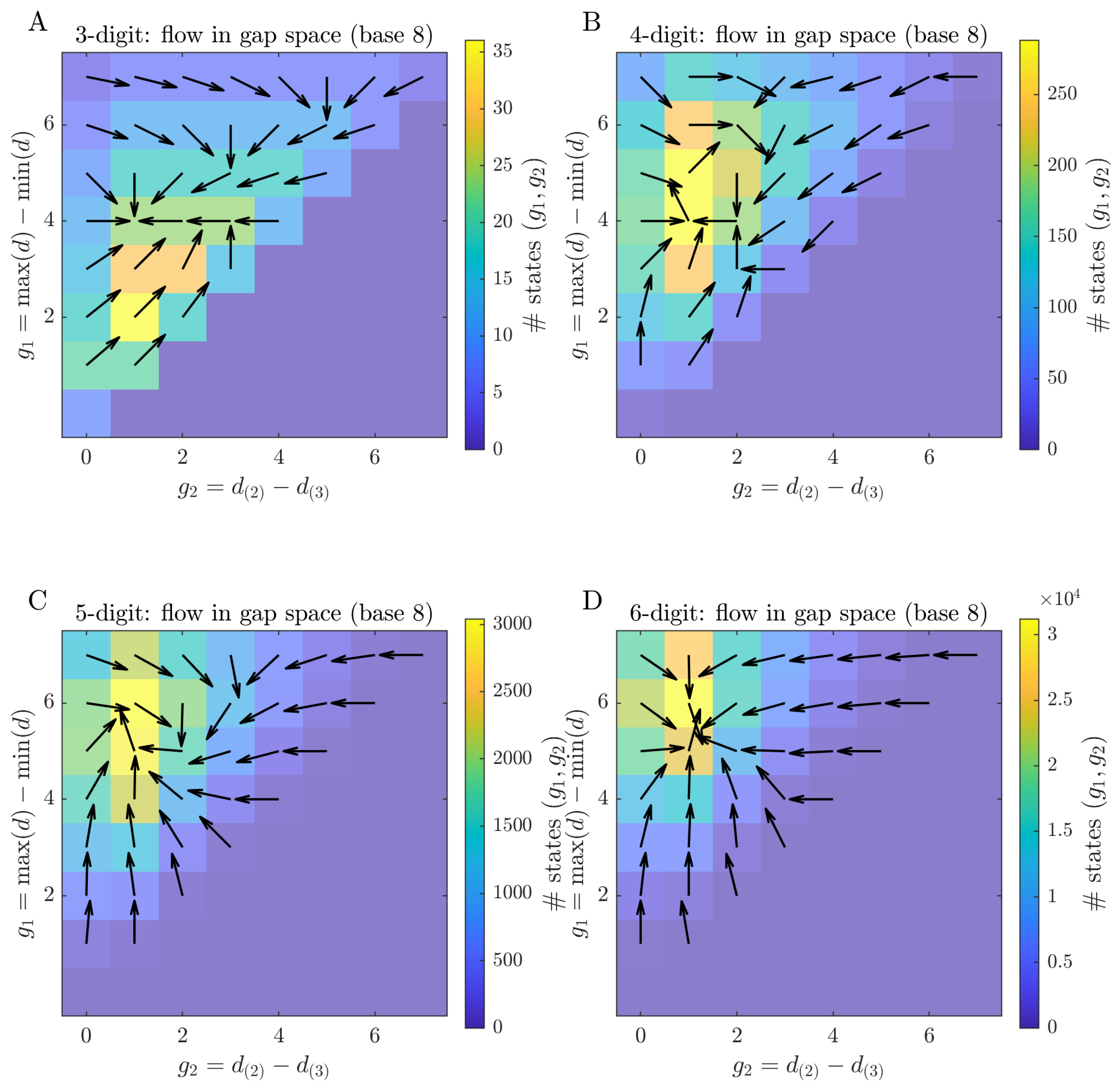
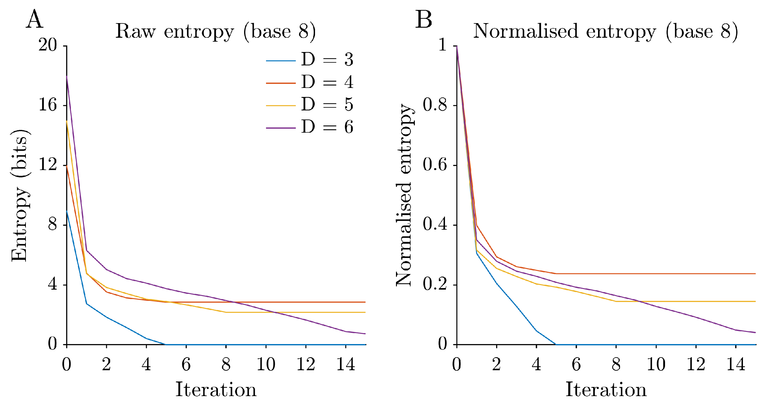
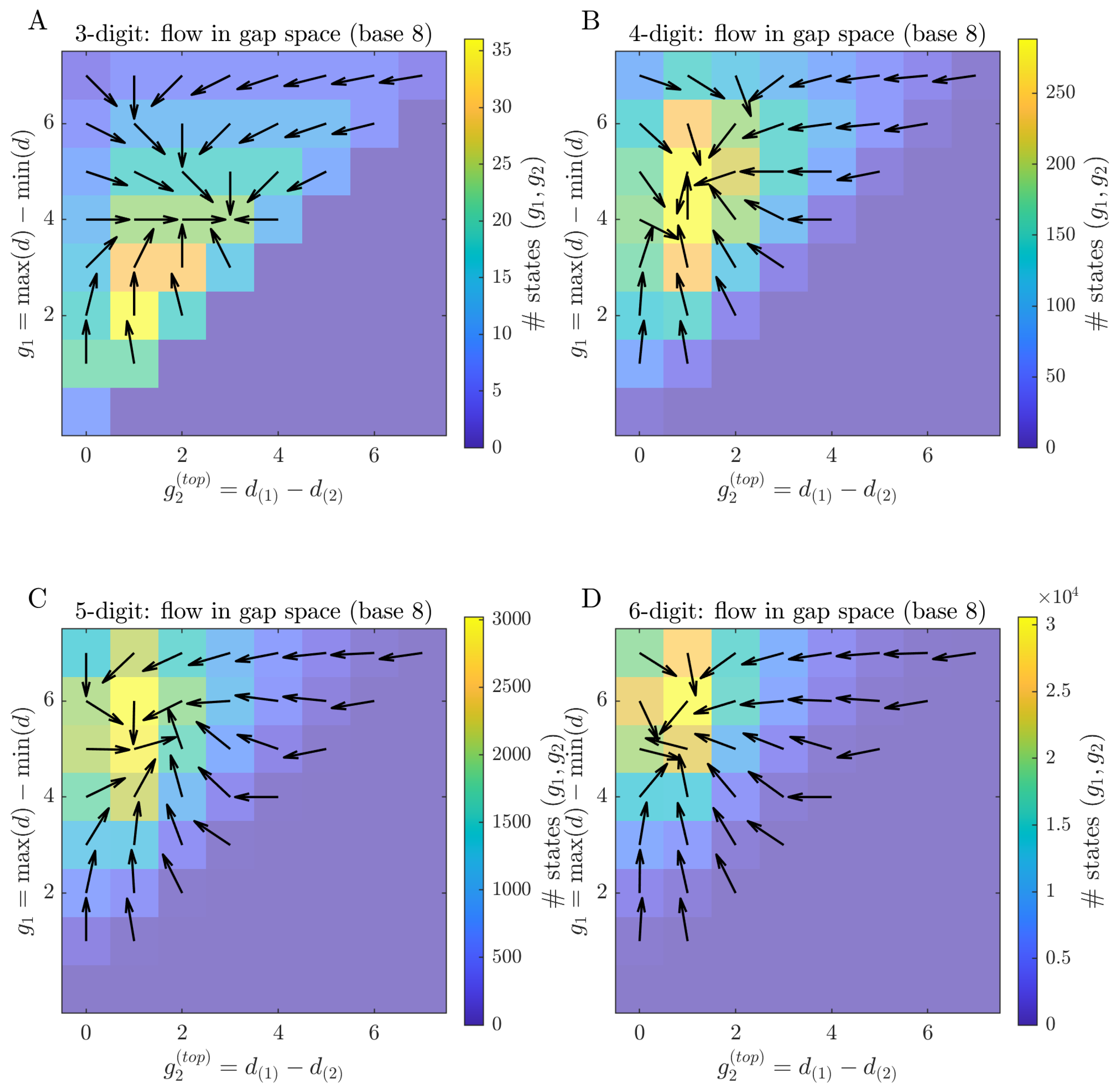
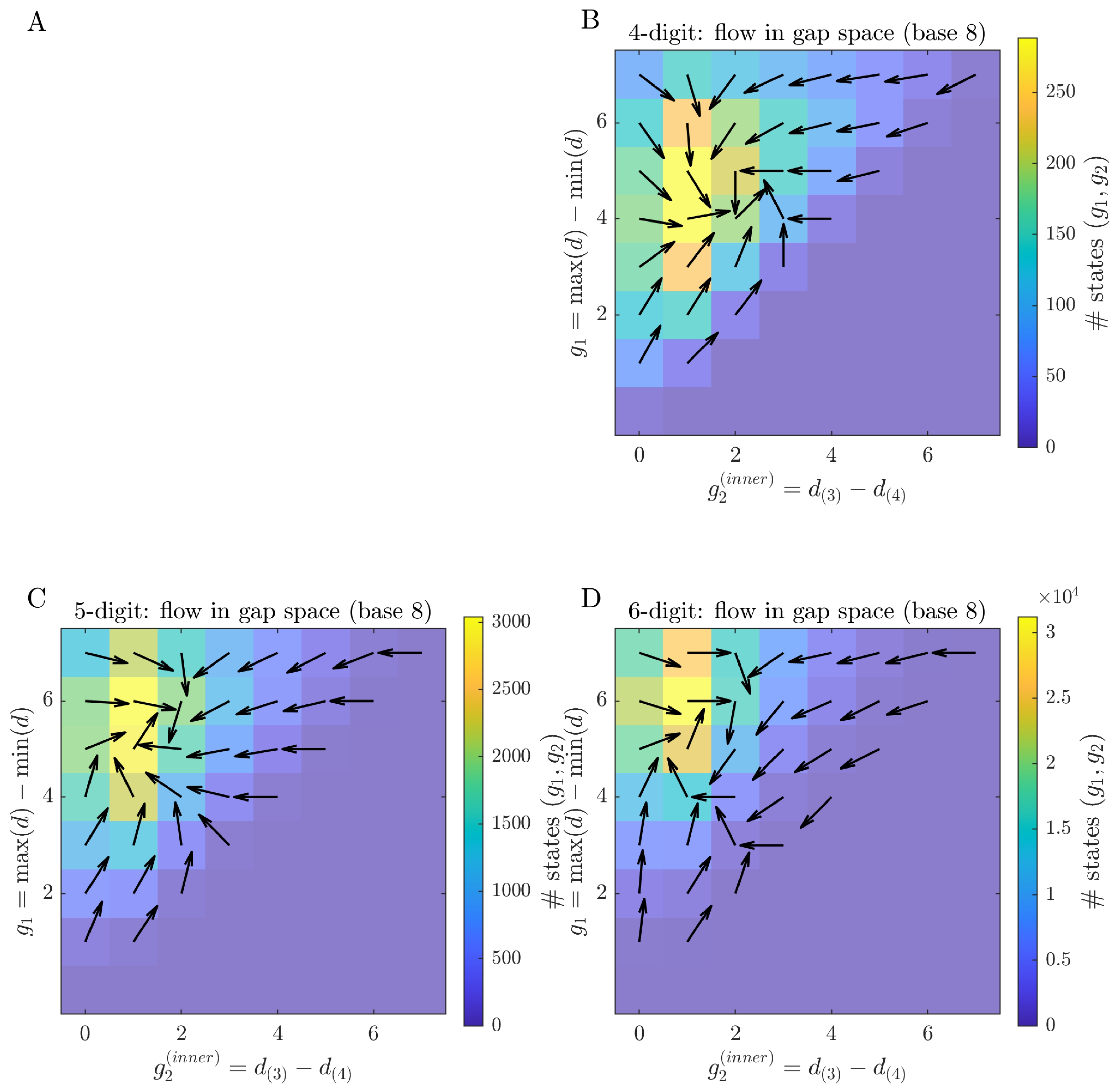
Appendix A.2 repeat selected analyses in base 8 to assess which qualitative conclusions are stable across bases.
Here a different angle is taken; instead of trying to obtain closed-form expressions for constants or loops, the Kaprekar map is treated as a finite directed graph, and questions are posed about its global statistics and coarse-grained descriptions: how entropy contracts, how permutation symmetries can be exploited, and how far simple ‘gap’ features go in explaining the dynamics. Standard tools from information theory and Markov-chain analysis [
14,
15,
16] are used. In the present work these questions are addressed for
by combining exhaustive enumeration with information-theoretic and statistical tools. The map
K in (
2) is treated as a deterministic update on a finite directed graph, and its structure is analysed at three complementary levels. First, at the level of individual states and attractors, all
D-digit states with at least two distinct digits are enumerated, their attractors and distances (numbers of iterations) to convergence are obtained, and basin sizes are quantified. This representation makes it possible to construct
entropy funnels: starting from a uniform distribution over states, the evolving distribution over attractors among the trajectories that have already converged is followed across iterations and the corresponding Shannon entropy is measured, providing a quantitative notion of uncertainty reduction under the dynamics. Second, the permutation symmetry of digit strings is exploited by grouping states into equivalence classes with identical digit multisets. This reduction yields a more compact representation that still respects the combinatorial constraints of the map. Multiset-level statistics are used to characterise how class sizes are distributed, how far typical classes lie from their attractors, and how different attractors are assembled from contributions of many small versus a few large classes. Third, a low-dimensional description is introduced in terms of simple digit-gap features. From the exact deterministic dynamics, empirical one-step transition frequencies between gap states can be estimated, yielding a first-order Markov approximation on this coarse-grained space. On this gap space, transition probabilities, stationary distributions, flow fields, and drift statistics are computed, and the resulting structure is related back to the basins and distances in the original state space. In addition, a simple linear regression framework is used to probe how far gap-based and aggregate digit features can account for the distance to attractor, viewed here as a notion of “difficulty” of reaching an attractor. All transition and stationary quantities reported for the gap-space chain are computed numerically from exhaustive enumeration; no closed-form derivation is claimed.
These three levels of description (states, multisets, and gap space) give a multiscale view of Kaprekar’s routine: from individual trajectories and basins to symmetry-reduced classes and finally to a very low-dimensional Markov approximation. The same approach should extend to other digit-based transforms and, more generally, to deterministic maps where one cares about coarse-grained information flow.
2. Materials and Methods
2.1. State Space, Attractors, and Distances
Fix a digit length
and work in base 10. Let
denote the set of
D-digit states with at least two distinct digits, allowing leading zeros. Throughout, states are represented as length-
D digit strings (in base 10) with
leading zeros allowed. Equivalently, each integer is padded to
D digits before applying the Kaprekar step (e.g., for
, 100 is treated as 0100). All digit sorting operations are performed on these
D digits, including any zeros. This convention, commonly adopted in the Kaprekar literature, ensures that
is closed under the map
. For each
D considered, restricting the initial ensemble to states without leading zeros does not change the attractor cycles reached or the entry times
for those states; it only changes the induced basin weights under a uniform prior, because the prior mass over
is altered. Write
as a
D-tuple of digits
. The descending and ascending orderings
and
are defined as in (
1), and the Kaprekar map is given by (
2). When restricted to digit length
D it is written as
.
Because is finite and is deterministic, every trajectory is eventually periodic: for each there exist integers and such that for all . Accordingly, an attractor is defined as a periodic orbit (cycle) of ; fixed points are the special case .
Lemma 1 (Eventual periodicity on a finite state space)
. Let be a function on a finite set S. Then for any the sequence is eventually periodic: there exist and such that for all .
Proof. Since S is finite, the sequence must repeat a value: there exist with . Let and . Determinism implies that for all . □
A periodic orbit (cycle) is an attractor if it is a directed cycle of : there exist and distinct states such that and for all i. Fixed points are the special case (then with ).
Given an attractor cycle
C, its (forward)
basin is
For
the
distance to attractor (cycle entry time) is defined as
It is convenient to write
for the attractor cycle reached from
x and
for the corresponding convergence time. The observed cycle structure for each
(including whether
occurs) is reported in
Section 2.2 and
Appendix A.3. For each
the set
is enumerated, all attractor cycles are identified, basin sizes
are computed, and
is recorded for all states.
2.2. Attractor Detection and Cycle Structure
For each digit length
D, the map
was iterated from every state
until the trajectory first revisited a previously visited state. From this first repeat, the resulting periodic orbit (cycle)
and its length
were extracted and recorded. For
and
, all attracting cycles had length one (fixed points). For
, all attractors were genuine cycles with
(one 2-cycle and two 4-cycles). For
, both fixed points (
) and a dominant 7-cycle (
) were observed. The full cycle lists, lengths, and basin weights are provided in
Appendix A.3.
2.3. Entropy Funnels
To quantify information funnels an initial distribution that is uniform over all non-trivial states for a given
D is considered. For each iteration
define the subset of states that have already reached an attractor by time
t,
Among these converged states, the empirical distribution over attractors at time
t is
where the sum over
a runs over all attractors for the given
D. The Shannon entropy
is then computed as a function of iteration
t. For small
t the distribution
is dominated by attractors that are reached quickly; as
t increases and more trajectories converge,
approaches the basin size distribution. Plotting
yields a raw entropy funnel. To compare decay profiles across
D, the normalised entropy is plotted,
where
denotes the basin size entropy, i.e., the entropy of the attractor distribution obtained once all states have converged (
, so that
and
), and in practice
is set to
with
in the computations. Thus
and
as
.
2.4. Multiset Representation
Because permuting the digits of x does not affect the outcome of a Kaprekar step, many states form equivalence classes with identical digit multisets. Formally, an equivalence relation is defined on by if their digits coincide as multisets. The equivalence classes are in bijection with digit multisets and are referred to as multiset classes. Each class has a size (number of distinct permutations) and a well-defined mean distance to attractor obtained by averaging over the states in the class. For each D all digit multisets, their class sizes, and their mean distances are enumerated. It is also recorded, for each attractor, how many states in its basin arise from each multiset class.
2.5. Gap Features and Markov Chain in Gap Space
To obtain a low-dimensional, permutation-invariant description of digit structure, two simple “gap” features are used (defined formally in Equation (
9)). The first captures overall digit spread, while the second captures an internal separation that distinguishes configurations in which one or two extreme digits are separated from a more homogeneous bulk. In preliminary exploratory work, additional quantities such as further internal gaps, digit sum, and digit variance were inspected. Digit sum and digit variance are later included as predictors in the regression analysis, but
are adopted for the Markov-chain description because they already generate a compact and interpretable gap space.
Appendix A.2 further compares induced occupancy and mean drift fields under alternative definitions of
, quantifying agreement via cellwise correlations and the mean cosine similarity of drift vectors.
For each state
simple digit features are computed. For notational convenience, let
denote the digits of
x sorted in non-increasing order (including leading zeros). The gap features used for the gap-space projection are defined as
Here
denotes the
k-th largest digit of
x.
The choice
is intended to capture an
internal break between the leading digits and the remaining digits. In particular, many digit configurations share the same overall spread
but differ in whether there are two extreme digits separated from a more homogeneous bulk; this distinction is directly reflected in
. By contrast, the alternative
primarily detects a single extreme digit and is therefore often partly redundant with
. To assess the robustness of the coarse-grained description,
Appendix A.2 compares the induced flow fields obtained from several alternative definitions of
and reports which qualitative conclusions are stable across choices.
These define a discrete set
of possible gap pairs
.
Because the projection is many-to-one, the induced dynamics on is generally non-deterministic: distinct digit strings sharing the same gap state g can transition to different successor gap states under the deterministic Kaprekar map . An empirical first-order Markov approximation on this discrete grid is therefore defined by counting one-step transitions across the exhaustively enumerated map.
For each gap state
, consider the collection of underlying states
One Kaprekar step is applied to each
, the successor gap state
is recorded, and empirical transition frequencies
are estimated.
Equivalently, letting , one has . The matrix is row-stochastic and summarises the average one-step behaviour of the full deterministic map after projection to the gap space.
A stationary distribution of the Markov approximation is any distribution on satisfying . In practice, the stationary distribution reported is obtained numerically by iterating until convergence from the initial gap distribution induced by the uniform prior on ; when the chain is ergodic, this is equivalent to computing the normalised left eigenvector of associated with eigenvalue 1.
For visualisation of gap-space flow fields, a drift vector is associated with each occupied gap state
. Writing
and
, the empirical mean one-step drift at
g is
Because
is exhaustively enumerated for each
, this average includes
all states
x consistent with the gap pair
g.
To quantify within-cell heterogeneity (i.e., how much
varies across different states
x sharing the same gap pair
g), the empirical covariance of increments is also computed,
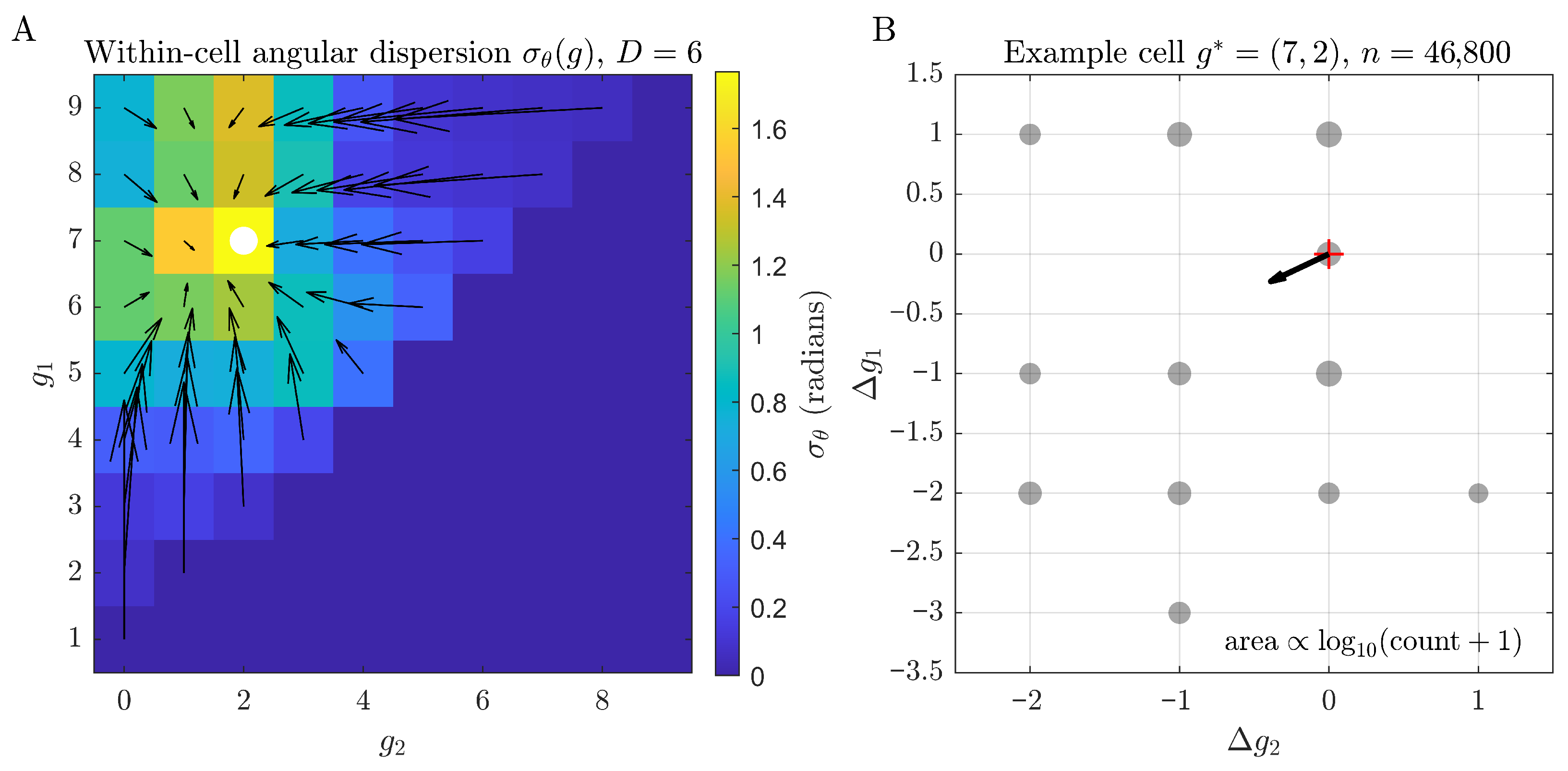
Appendix A.1 reports representative examples and summary dispersion statistics, providing a direct visualisation of variability around the mean drift arrows.
These empirical probabilities define a first-order Markov chain on with transition matrix , which provides a coarse-grained approximation to the projected dynamics on the gap space (the true projected process need not be strictly Markov). It should be emphasised that is used here as a descriptive first-order approximation to the projected dynamics on the gap space. Quantifying the approximation error (e.g., by comparing against higher-order models) is an important direction but is beyond the scope of the present work. The chain is therefore treated primarily as a compact summary of average flow patterns rather than an exact probabilistic model of the projected dynamics. The following quantities are computed: (1) the stationary distribution satisfying (computed numerically, e.g., as the normalised left eigenvector of or by power iteration); (2) the empirical distribution of gap states under the uniform prior on ; and (3) average changes and per step for each gap state.
2.6. Predicting Distance to Attractor from Digit Features
To link local digit structure to distance to attractor, a simple regression analysis is performed. For each
D, up to
N = 50,000 states (or all states when fewer are available) are drawn uniformly without replacement from
. For
this corresponds to a random sample of approximately
of all admissible states, which keeps computation manageable while still covering a wide range of digit configurations. For each sampled state,
and
as defined above, the mean digit
, and the variance of digits
are computed. All reported goodness-of-fit metrics are computed on held-out test data: for each
D, the sampled states were split into
training and
test sets, the model in (
15) was fit on the training set, and
and RMSE were evaluated on the test set. All features are standardised (zero mean and unit variance). The mean digit
is used instead of the raw digit sum to remove trivial scaling with
D. A linear model
is then fit by least squares, and, for each
D, the coefficient of determination
, the root mean squared error (RMSE), and the learned weights
are reported. For the comparisons between “easy” and “hard” states in
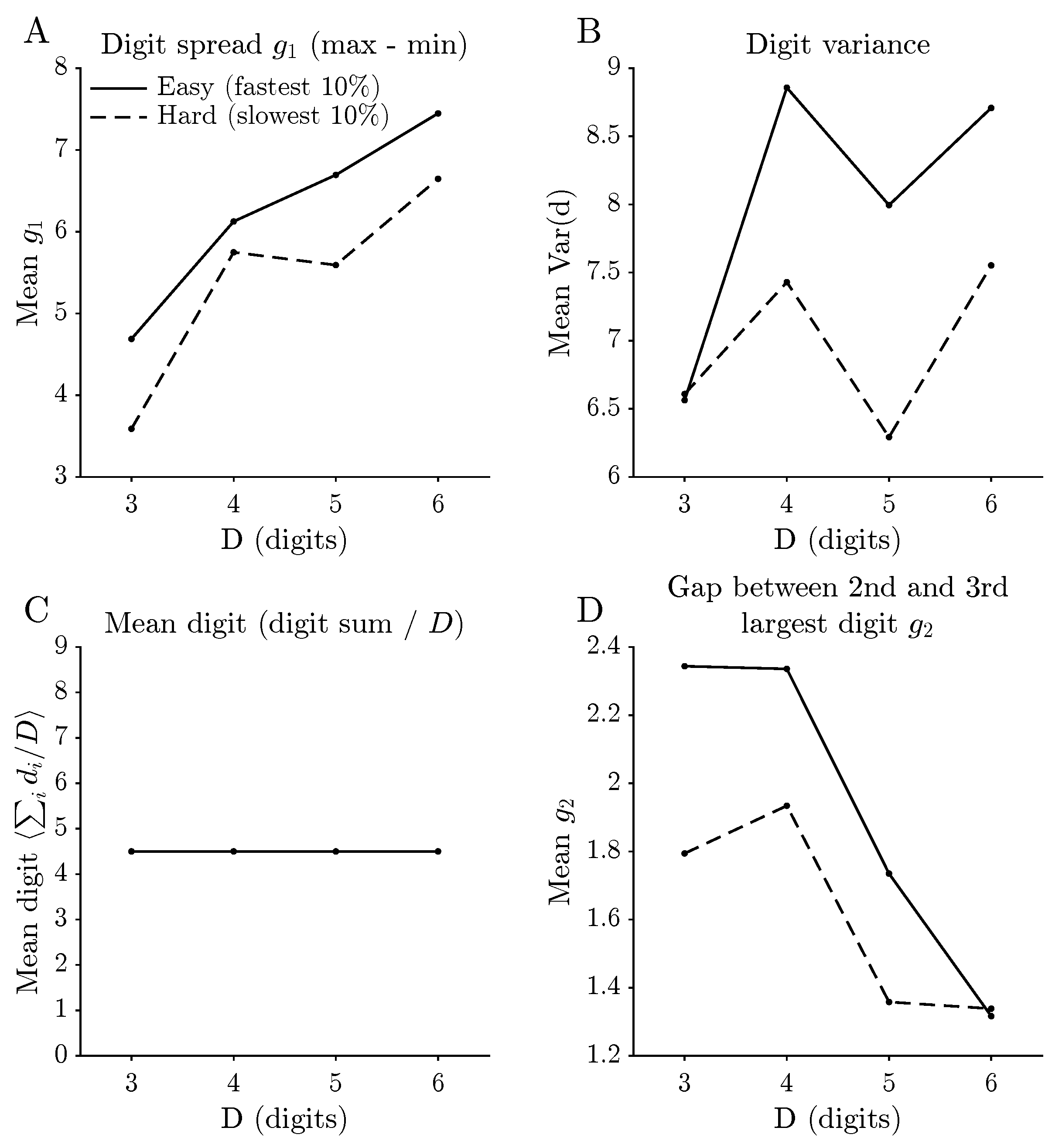
Figure 1, states are ranked by
and the fastest and slowest deciles (smallest and largest
of distances) are selected. Digit features are then averaged separately for these two groups. Throughout this subsection, linear regression is used deliberately as a simple and interpretable baseline. The model links distance to attractor to low-dimensional digit summaries in a way that allows direct inspection of feature weights and effect directions, at the cost of restricting attention to linear relationships. More flexible nonlinear models (e.g., decision trees or kernel-based methods) could in principle capture additional structure in the data but would make it harder to relate predictive performance back to specific digit features. For this reason, the present analysis treats the linear model as a reference point rather than an attempt to optimise predictive accuracy.
2.7. Numerical Setup
All computations were performed in MATLAB (R2024b, Mathworks®, Natick, MA, USA), using integer-valued operations for the Kaprekar map that are exactly represented in double-precision arithmetic for the ranges of D considered and double-precision arithmetic for derived quantities such as entropies. Enumeration of and construction of the gap-space Markov chain are exact for each . Where sampling is used (in the regression analysis), the corresponding sample size is stated.
4. Discussion
The results above describe Kaprekar’s routine, for
–6, as a finite dynamical system seen through several information-theoretic lenses. A very simple digit transform already produces a surprisingly layered structure: shallow typical transients but long tails, a shift from one dominant basin to many smaller ones, and a useful, but ultimately limited, low-dimensional gap description. At the coarsest level, the global summaries in
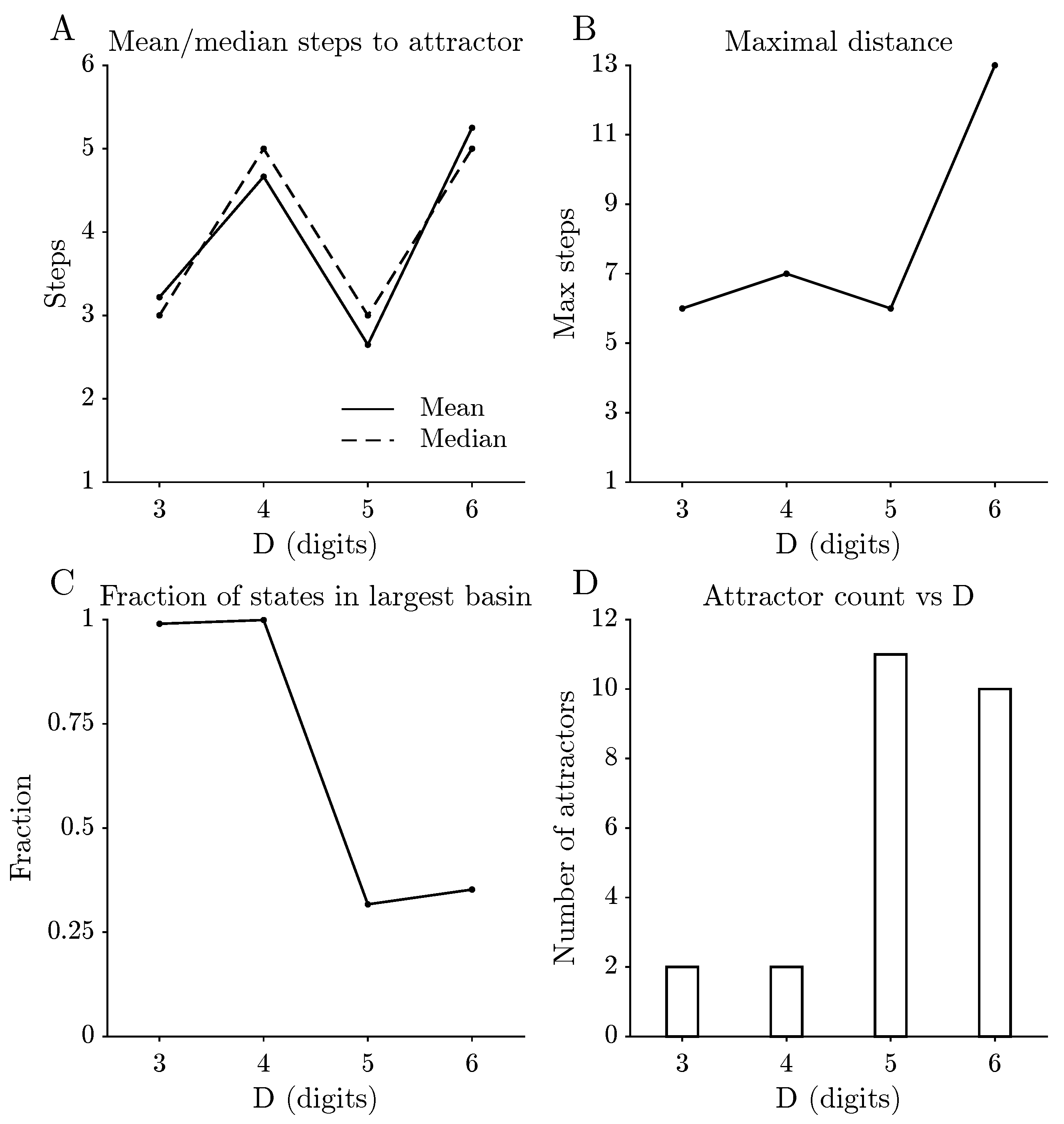
Figure 3 indicate that the Kaprekar dynamics remains shallow on average across all digit lengths considered: typical trajectories reach an attractor in only a few iterations, despite the combinatorial growth of the state space. This shallow behaviour coexists with marked changes in extremal and structural quantities. The maximal distance to attractor increases with
D, the dominance of the largest basin decreases, and the number of distinct attractors rises. For three and four digits, the dynamics are effectively governed by a single large basin, whereas for five and six digits the state space splits into many smaller basins with more heterogeneous sizes. This transition from “one big funnel” to a more fragmented landscape is a first indication that, within the range
–6 examined here, the global organisation of the map shifts from dominance by a single large basin to a heterogeneous collection of smaller basins. The entropy funnels in
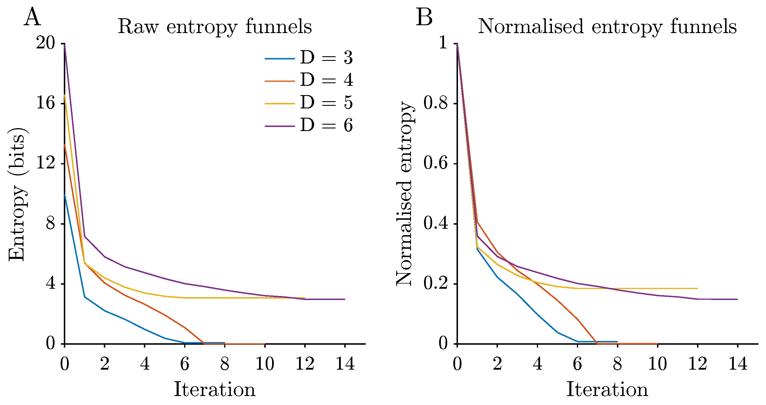
Figure 4 provide a complementary information-theoretic view. Starting from a uniform prior over states, the induced distribution over attractors among the trajectories that have converged exhibits a rapid initial entropy drop, followed by a slower tail. In more concrete terms, most uncertainty about the eventual attractor is resolved within a handful of iterations, but a small residual uncertainty can persist for many steps, especially when many attractors of comparable basin size are present. For
and
, the normalised entropy curves fall close to zero, in line with the near-monopolisation of the state space by a single attractor. For
and
, the residual entropy remains appreciable, reflecting the proliferation of attractors and a more even spread of basin sizes. Thus, entropy funnels capture, in a single scalar time series, both the fast collapse of uncertainty and the dependence of long-term behaviour on basin geometry.
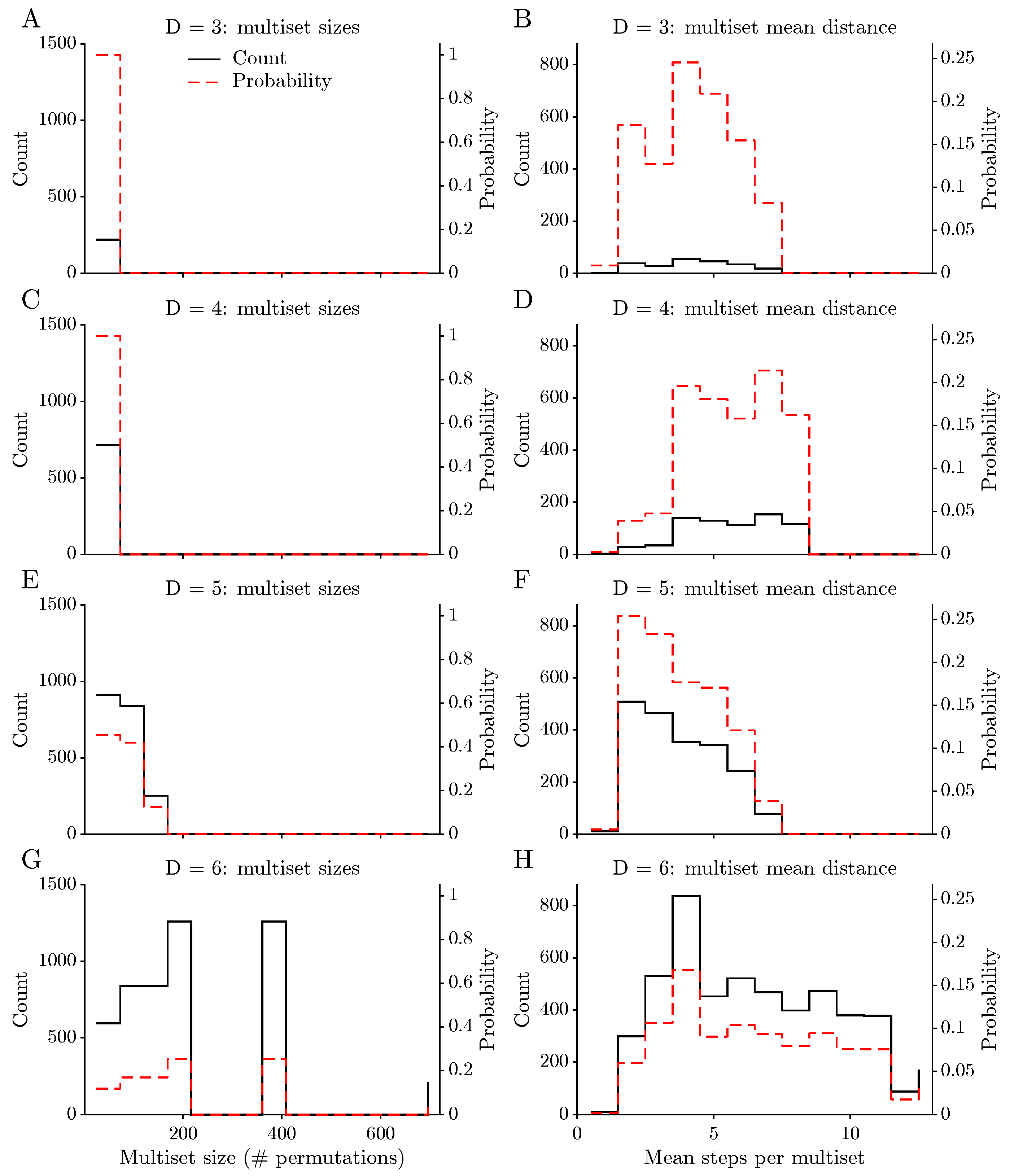
Factoring states into digit multisets yields a first level of symmetry reduction that separates combinatorial and dynamical effects (
Figure 5). On the combinatorial side, both the number of multiset classes and their typical sizes grow quickly with
D, and the size distributions develop heavier upper tails. This indicates the appearance of rare digit patterns that admit many distinct permutations. On the dynamical side, the distributions of mean distance to attractor per multiset remain concentrated on short distances but develop longer tails for
and
. A small subset of multisets is therefore systematically associated with longer transients. In other words, as
D increases the basin structure is distributed more unevenly across multisets: a few digit patterns dominate large basins, while many others sit in small, long-tailed classes. The analysis of “easy” and “hard” states in
Figure 1 moves one step closer to the digit level. By contrasting the fastest and slowest deciles of distance to attractor, simple patterns emerge: easy states tend to have a larger overall digit spread
and, for some digit lengths, higher digit variance. Configurations whose digits are widely dispersed therefore tend, on average, to reach an attractor more quickly. In contrast, the total digit sum carries much less interpretable dynamical information once trivial scaling with
D is taken into account. These observations suggest that certain aspects of “difficulty” are already visible in low-level digit statistics, even before more refined features are introduced.
Gap space provides a coarser, but highly structured, view of the dynamics. By tracking only the overall spread
and the internal gap
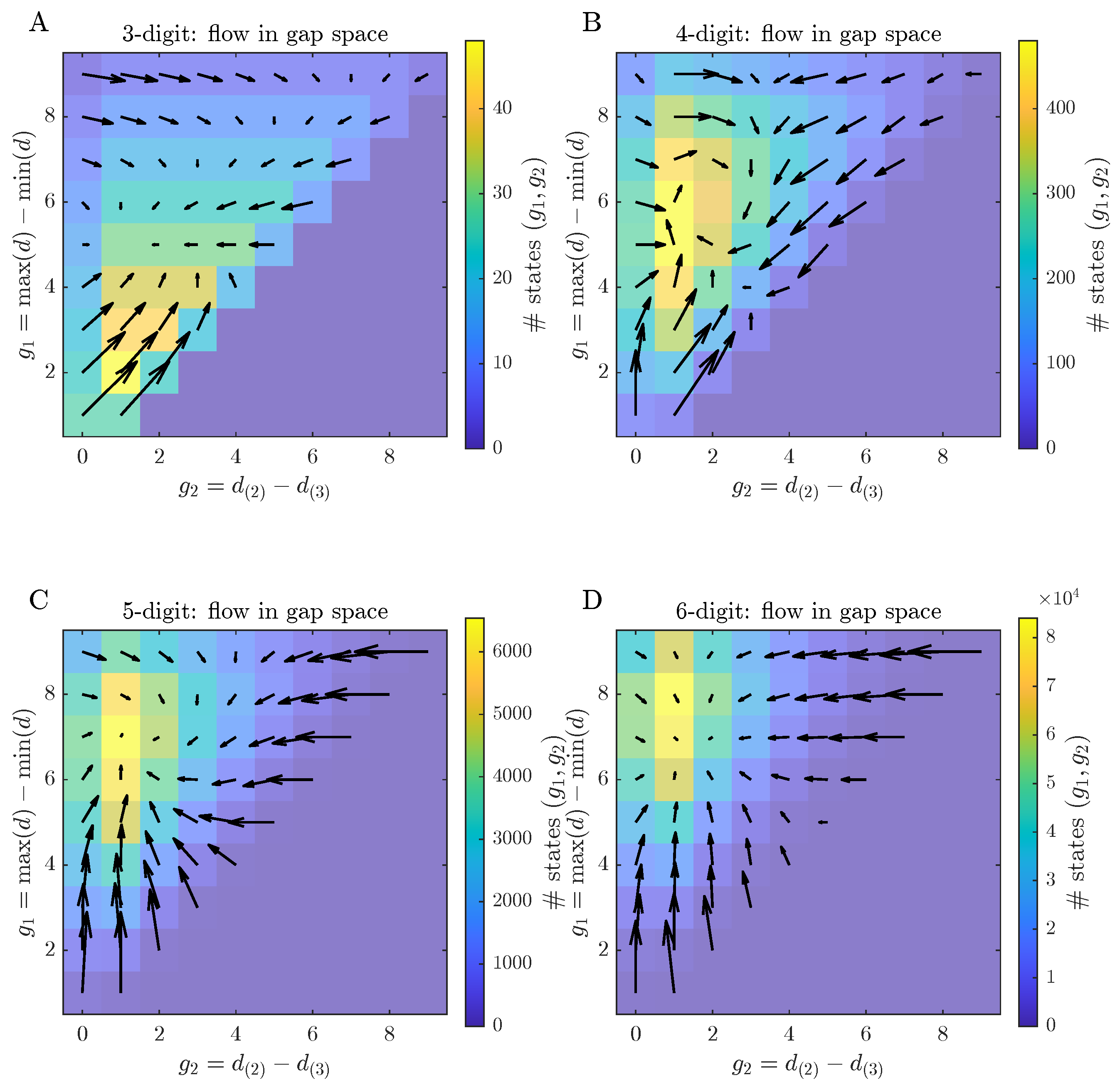
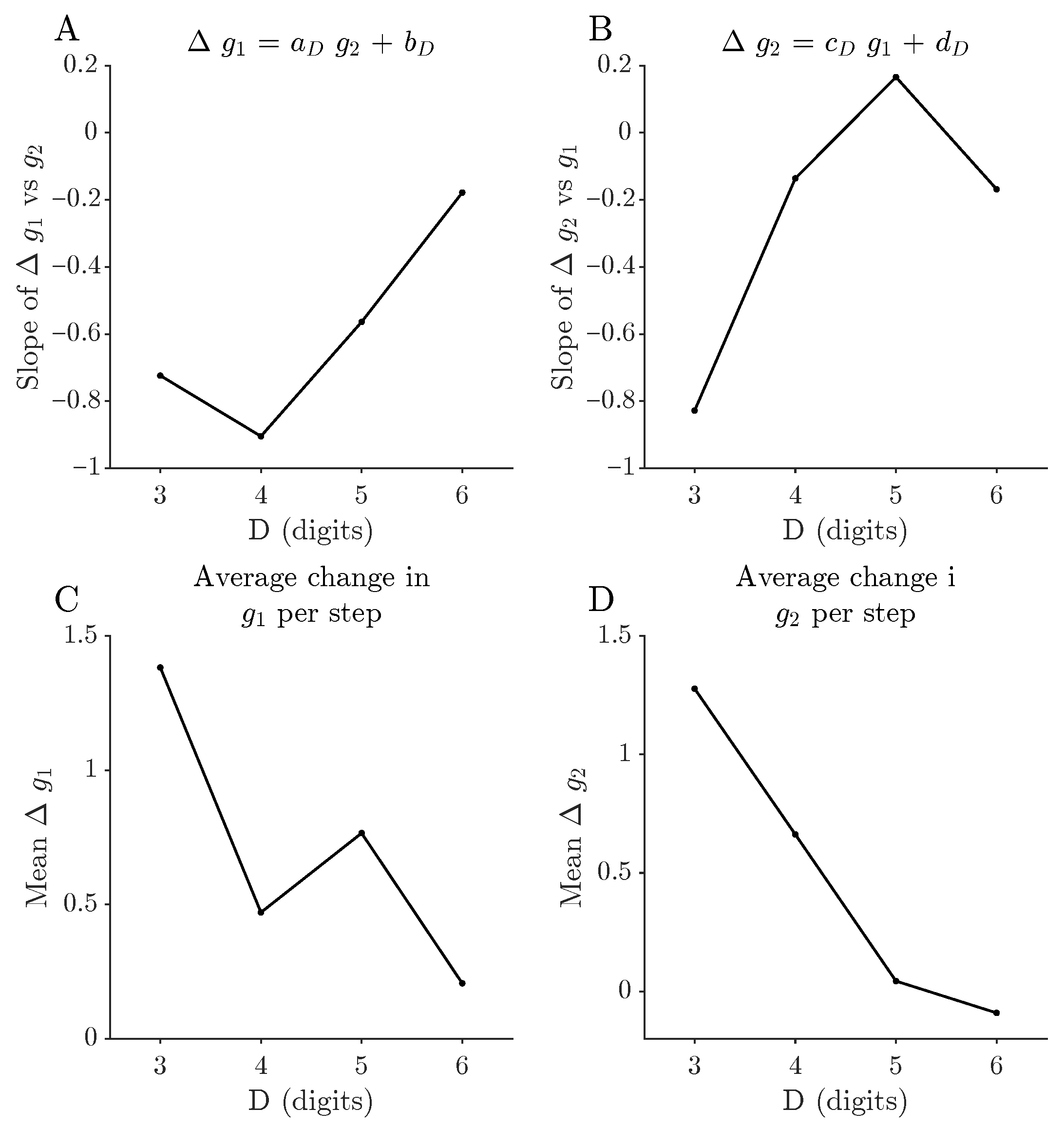
between the second and third largest digits, Kaprekar’s routine induces an empirical first-order Markov chain on a relatively small grid. The resulting flow fields and drift statistics reveal a consistent directional bias: on average, one Kaprekar step tends to increase
and decrease
, pushing states towards regions with a wide overall digit range but a more balanced configuration among the middle digits (
Figure 6). For three digits, successor states concentrate near the diagonal
, and the coupling between
and
is strong. As
D increases, the stationary distributions shift and the linear relations between
and
, and between
and
, weaken in slope. This weakening suggests that, in higher-digit systems, the two gap coordinates no longer suffice to capture the dominant directions of flow and that additional degrees of freedom in the digit space become dynamically relevant. The gap-space Markov chain is therefore best viewed as a first-order coarse-grained description: it captures the main flow patterns in
but is not intended as an exact probabilistic model of the projected dynamics. The regression analysis in
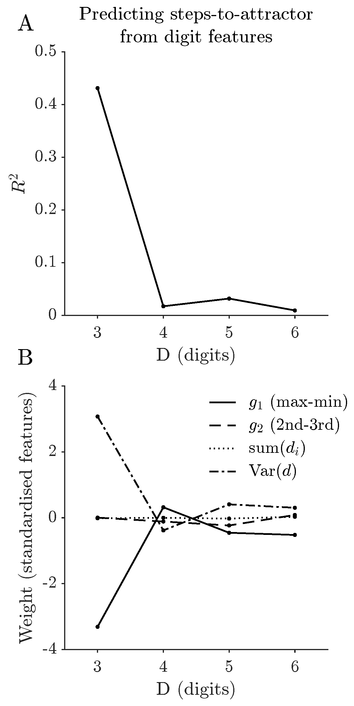
Figure 7 makes this limitation explicit. For
, a simple linear model based on
explains a substantial fraction of the variance in distance to attractor, with errors on the order of one step. In this regime, low-dimensional digit summaries provide a reasonably informative proxy for dynamical difficulty. For
, however, the coefficient of determination
drops to a few percent and the learned feature weights shrink and fluctuate in sign. Beyond three digits, the relationship between local digit structure and global convergence time becomes increasingly high-dimensional and entangled, so that linear combinations of a small number of simple features capture only a small part of the behaviour. This breakdown of low-dimensional predictability within the present feature set is consistent with the more fragmented basin geometry and more heterogeneous multiset patterns observed at larger
D.
Several limitations and extensions follow naturally from these findings. The present study is numerical and restricted to base 10 and digit lengths up to six. From a mathematical perspective, one natural direction is to seek analytic bounds on entropy decay, basin sizes, or gap-space drift as D grows, perhaps by exploiting known structural results on Kaprekar constants and loops in higher bases. Another direction is to refine the coarse-graining schemes: alternative feature sets, nonlinear mappings into the gap space, or higher-order Markov projections could be explored to recover part of the predictive power lost at larger D. The regression framework could also be extended beyond linear models, for example by investigating whether low-depth decision trees or other simple classifiers find more informative digit combinations without sacrificing interpretability.
More broadly, the picture that emerges is that of a finite information-processing system that rapidly funnels a large set of inputs into a much smaller set of outputs while retaining enough internal structure to defeat simple low-dimensional representations of the dynamics once the state space becomes sufficiently large. Kaprekar dynamics therefore offer a useful model system for studying information funnels and coarse-grained Markov structure in deterministic maps on finite spaces. Similar patterns occur in other settings: in statistical physics, many microscopic configurations are summarised by a few macroscopic variables, such as temperature or magnetisation [
17,
18]; in machine learning, deep networks and information bottleneck methods restrict information flow through low-dimensional latent or bottleneck layers, yielding compact internal codes that still support accurate predictions [
19,
20]; and in decision neuroscience, multiple streams of evidence are modelled as being accumulated into a single decision variable that governs choice [
21,
22,
23]. Against this background, the Kaprekar map provides a fully tractable model system: the entire state space and all attractors are known explicitly, yet the induced information funnels and coarse-grained dynamics remain non-trivial. This makes the Kaprekar map a natural model system for testing methods that search for informative coarse-grainings or low-dimensional summaries and for exploring how such techniques might carry over to more biologically motivated dynamical models.