
Harmonic Aggregation Entropy: A Highly Discriminative Harmonic Feature Estimator for Time Series


Abstract
1. Introduction
- (1)
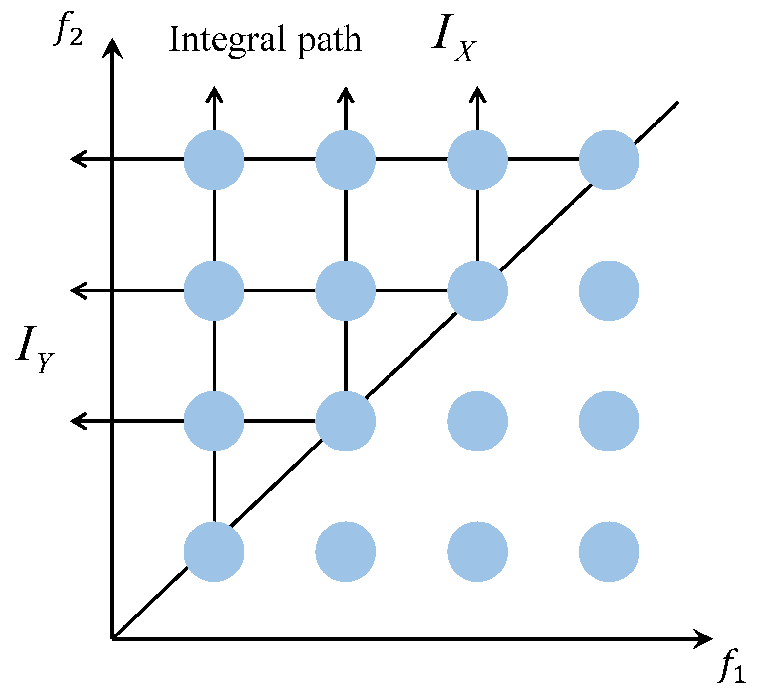
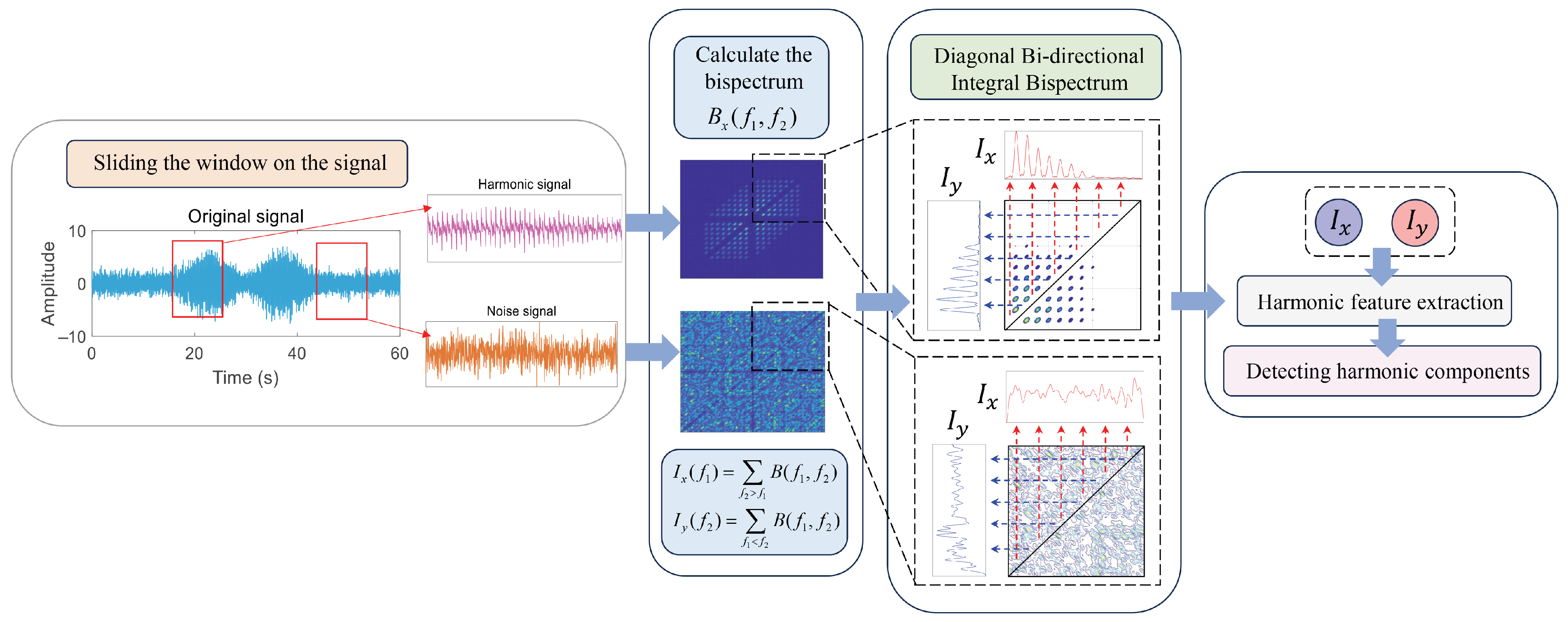
- A new bispectral integration method is proposed that utilizes the frequency coherence of harmonics to project features onto different frequency axes and addresses the issues of complex computation and feature redundancy in directly extracting features from the bispectrum matrix.
- (2)
- Based on DBIB, a new entropy theory is proposed to evaluate the consistency of integration results across two frequency axes by calculating their cross-entropy. The stronger the consistency, the smaller the entropy value, making the harmonics more prominent. Compared with other entropy measures, this method demonstrates greater discrimination and sensitivity to harmonics.
- (3)
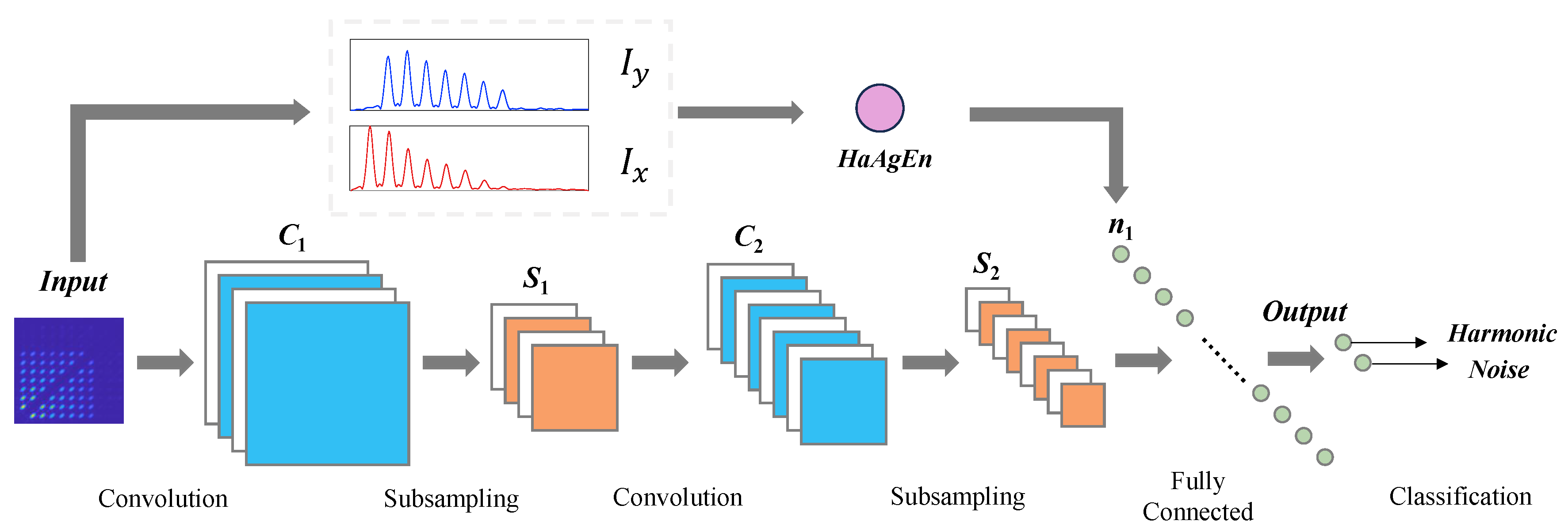
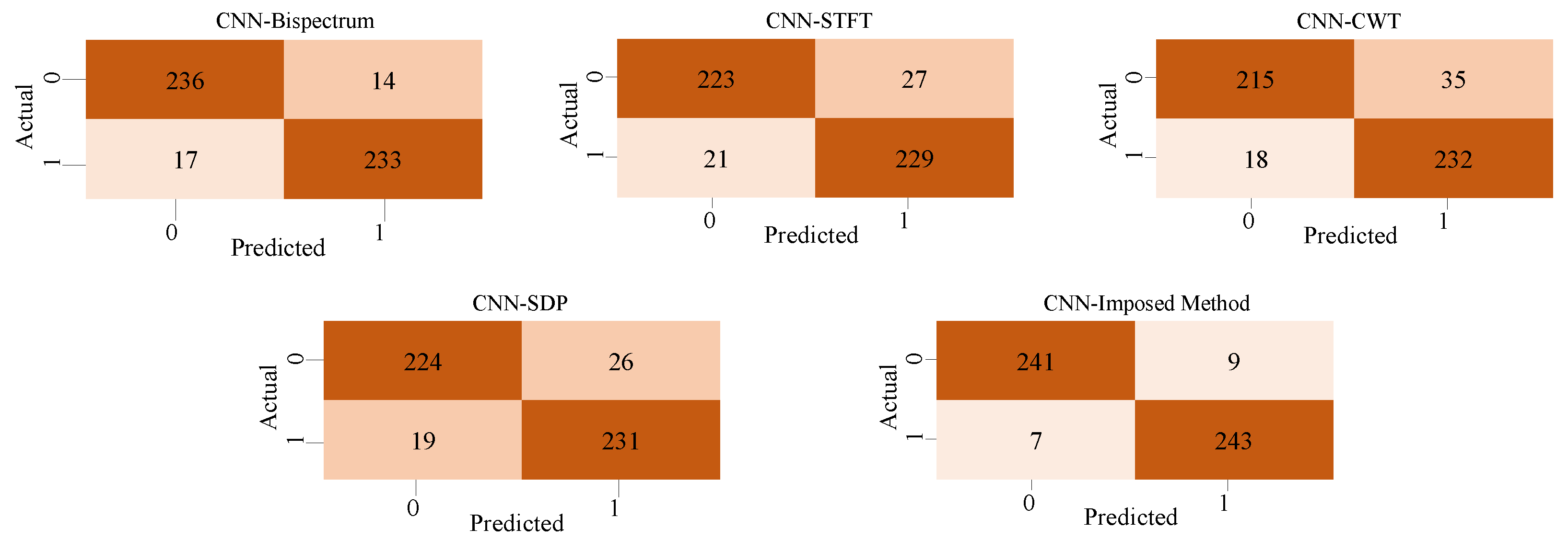
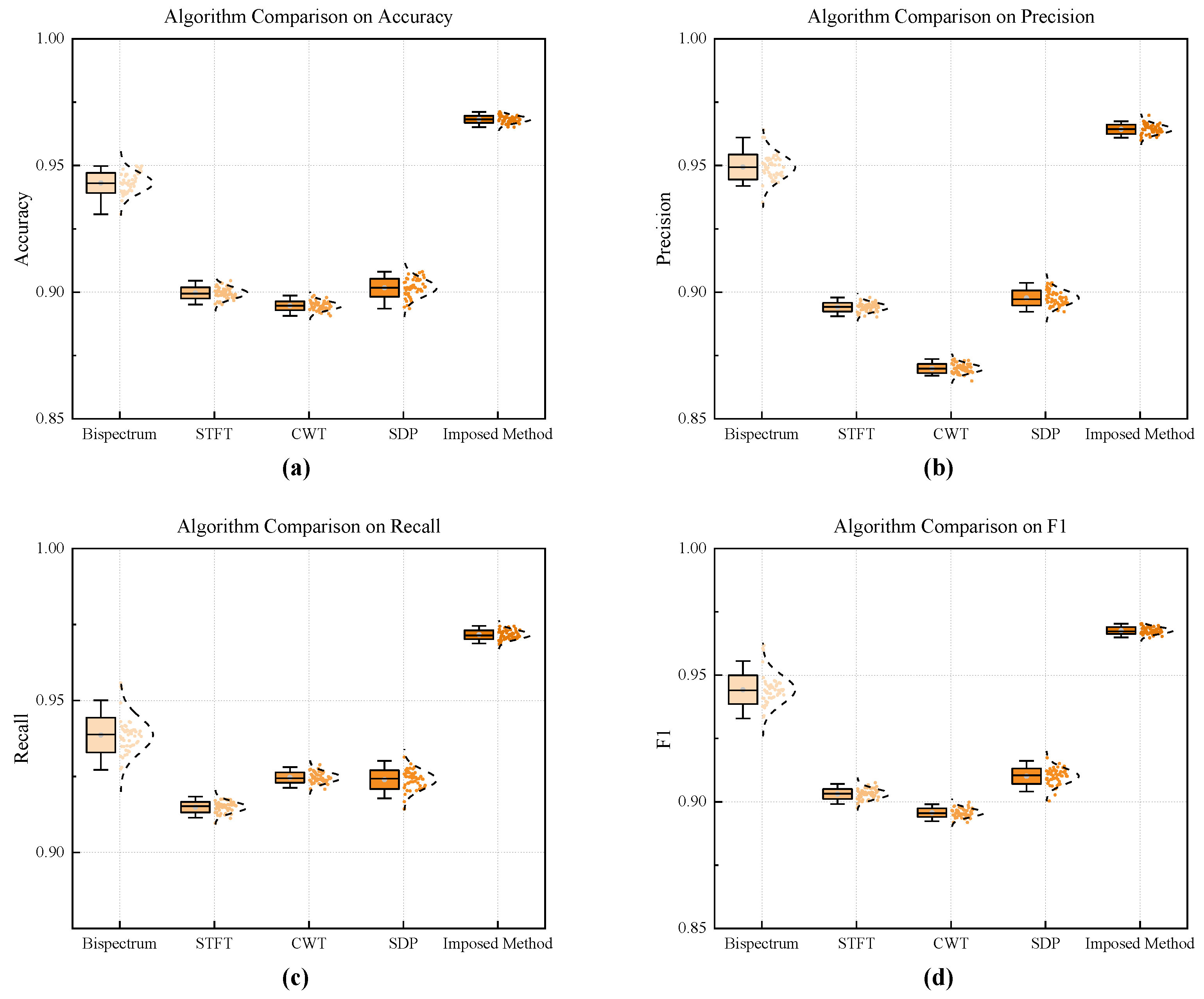
- HaAgEn is combined with a convolutional neural network to verify its effectiveness in the harmonic signal measured in the sea trial. Compared with other harmonic detection methods, the detection accuracy of the proposed method is significantly improved, reaching 96.8%.
2. Methodology
2.1. Bispectrum Analysis
- Represents the mathematical expectation, which is typically replaced by time averaging or segment averaging in practical applications.
- Represents the conjugate of X.
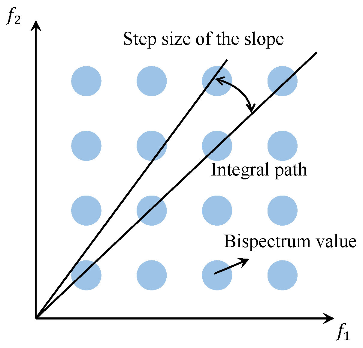
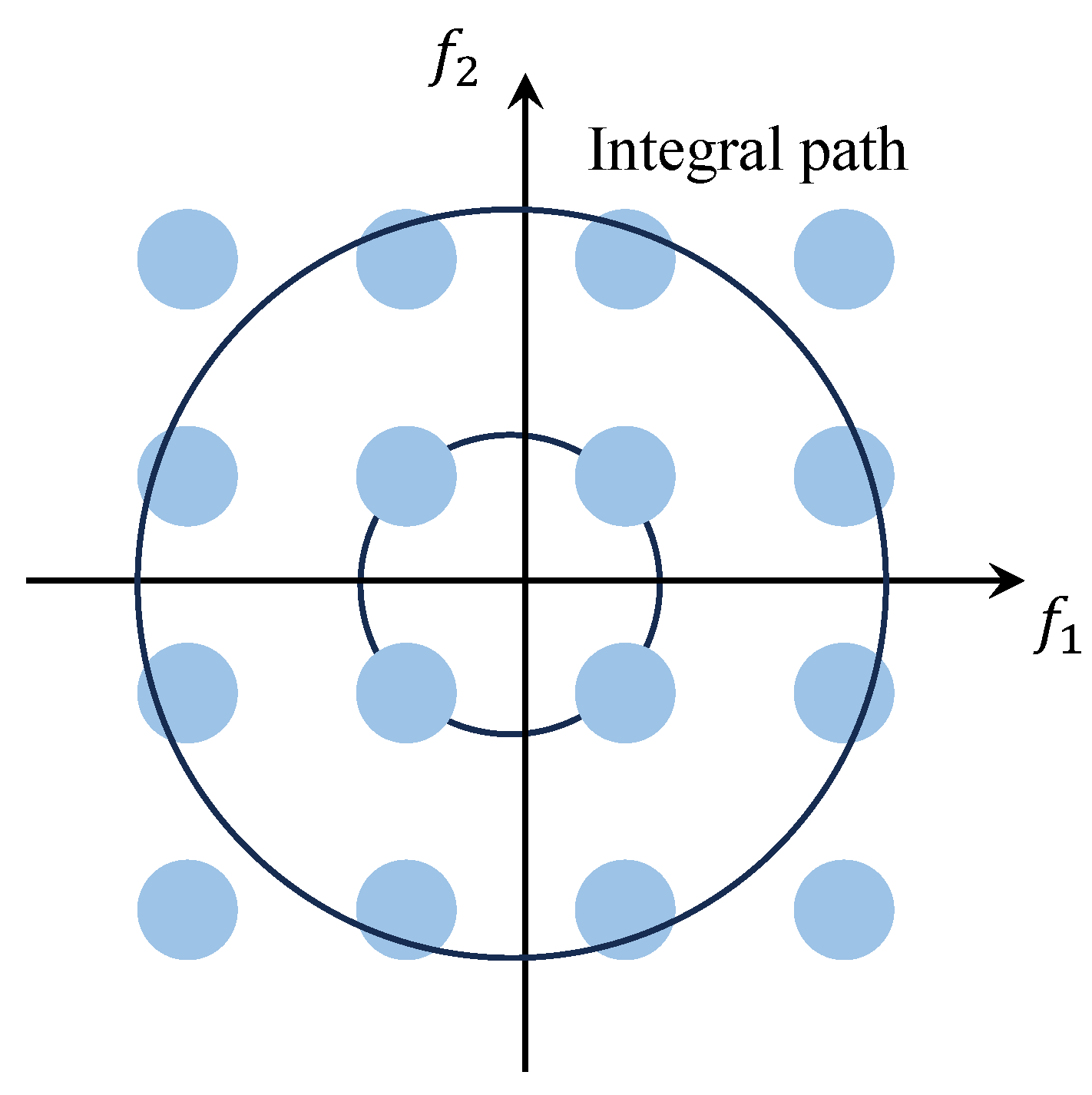
2.2. Integrated Bispectrum
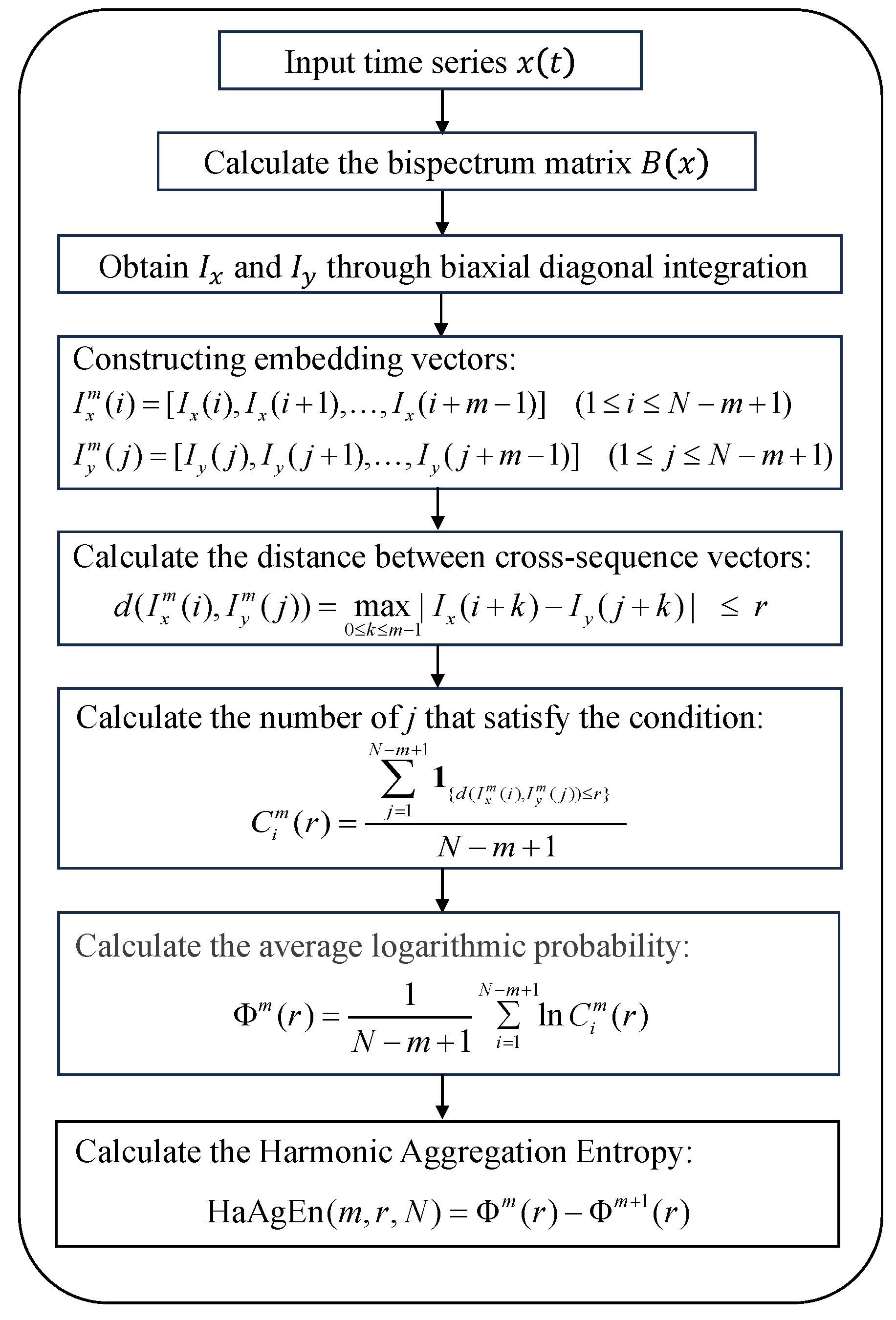
2.3. Harmonic Aggregation Entropy
3. Simulation Analysis
4. Sea Trial Data Validation
5. Conclusions
- (1)
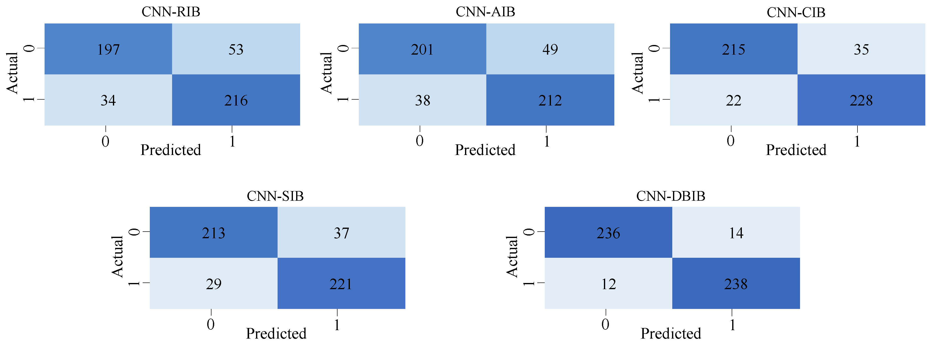
- To address the issue where existing bispectral integration methods cannot effectively extract harmonic features from time series, an innovative use of the frequency coupling characteristics of harmonic signals in the bispectral matrix was employed, leading to the proposal of the DBIB integration method. This method significantly outperformed other integration methods in comparative experiments and served as a foundation for further developing HaAgEn.
- (2)
- To address the situation where various types of entropy values cannot effectively characterize harmonic features in signals, further calculations were performed on the bispectral integration results based on DBIB, resulting in the HaAgEn of the time series. This was compared with various other types of entropy in experiments, demonstrating that its sensitivity to harmonics is significantly superior to other methods.
- (3)
- By integrating HaAgEn with convolutional neural networks, the method proposed in this paper significantly outperforms traditional methods of detecting harmonics using time–frequency feature inputs, such as STFT and CWT, especially within real maritime measurement datasets, achieving a detection accuracy of 96.8%.
Author Contributions
Funding
Institutional Review Board Statement
Data Availability Statement
Conflicts of Interest
References
- Queiroz, A.; Coelho, R. Harmonic Detection from Noisy Speech with Auditory Frame Gain for Intelligibility Enhancement. IEEE/ACM Trans. Audio Speech Lang. Process. 2024, 32, 2522–2531. [Google Scholar] [CrossRef]
- Birsan, M. Measurement of the extremely low frequency (ELF) magnetic field emission from a ship. Meas. Sci. Technol. 2011, 22, 085709. [Google Scholar] [CrossRef]
- Kim, Y.; Lee, S.; Kim, J. Influence of anode location and quantity for the reduction of underwater electric fields under cathodic protection. Ocean Eng. 2018, 163, 476–482. [Google Scholar] [CrossRef]
- Wang, D.; Yang, L.; Ni, L. Performance and harmonic detection algorithm of phase locked Loop for parallel APF. Energy Inform. 2024, 7, 25. [Google Scholar] [CrossRef]
- Xu, M.; Sang, Z.; Li, X.; You, Y.; Dai, D. An Observer-Based Harmonic Extraction Method with Front SOGI. Machines 2022, 10, 95. [Google Scholar] [CrossRef]
- Selvajyothi, K.; Janakiraman, P.A. Extraction of Harmonics Using Composite Observers. IEEE Trans. Power Deliv. 2008, 23, 31–40. [Google Scholar] [CrossRef]
- Yang, J.; Yu, C.; Liu, C. A New Method for Power Signal Harmonic Analysis. IEEE Trans. Power Deliv. 2005, 20, 1235–1239. [Google Scholar] [CrossRef]
- He, W.; Zhang, J.; Yao, W.; Tang, L. FFT-based Amplitude Estimation of Power Distribution Systems Signal Distorted by Harmonics and Noise. IEEE Trans. Ind. Inform. 2017, 10, 95. [Google Scholar]
- Daniel, K.; Kütt, L.; Iqbal, M.N.; Shabbir, N.; Raja, H.A.; Sardar, M.U. A Review of Harmonic Detection, Suppression, Aggregation, and Estimation Techniques. Appl. Sci. 2024, 14, 10966. [Google Scholar] [CrossRef]
- Wang, X.; Wang, B.; Wang, W.; Yu, M.; Wang, Z.; Chang, Y. Harmonic signal extraction from chaotic interference based on synchrosqueezed wavelet transform. Acta Phys. Sin. 2015, 64, 100201. [Google Scholar]
- Liu, L.; Zhi, Z.; Yang, Y.; Shirmohammadi, S.; Liu, D. Harmonic reducer fault detection with acoustic emission. IEEE Trans. Instrum. Meas. 2023, 72, 3522812. [Google Scholar] [CrossRef]
- Kumaraswamy, B. An Improved Sub-Harmonic to Harmonic Ratio Method for Pitch Estimation and Shadja Detection. Concurr. Comput. Pract. Exp. 2023, 35, 7604. [Google Scholar] [CrossRef]
- Hu, Y.; Zhu, Z.; Liu, K. Current Control for Dual Three-Phase Permanent Magnet Synchronous Motors Accounting for Current Unbalance and Harmonics. IEEE J. Emerg. Sel. Top. Power Electron. 2014, 2, 272–282. [Google Scholar]
- Zhu, Z.; Xu, M.; Li, P.; Wang, Q.S. Rapid Harmonic Detection Scheme Based on Expanded Input Observer. Electronics 2022, 11, 2860. [Google Scholar] [CrossRef]
- Zhang, J.; Wang, K.; Yang, D.; Yuan, Y.; Yang, S. Nonlinear Vibro-Acoustic Modulation for Microcrack Detection of Steel Strands Based on S-Transform Bispectrum. Appl. Acoust. 2025, 227, 110237. [Google Scholar] [CrossRef]
- Wilkinson, W.A.; Cox, M.D. Discrete Wavelet Analysis of Power System Transients. IEEE Trans. Power Syst. 1996, 11, 2038–2044. [Google Scholar] [CrossRef]
- Lu, Y.; Li, B.; Teng, G.; Zhang, Z.; Xu, X. A harmonic current detection algorithm for aviation active power filter based on generalized delayed signal superposition. Sci. Rep. 2025, 15, 10435. [Google Scholar] [CrossRef]
- Cichocki, A.; Lobos, T. Artificial neural networks for real-time estimation of basic waveforms of voltages and currents. IEEE Trans. Power Syst. 1994, 9, 612–618. [Google Scholar] [CrossRef]
- Sun, H.; Wang, L.; Qi, L.; Yan, J.; Jiang, M. Composite Harmonic Source Detection with Multi-Label Approach Using Advanced Fusion Method. Electronics 2024, 13, 1275. [Google Scholar] [CrossRef]
- Gao, X.; Liao, L. A New One-Layer Neural Network for Linear and Quadratic Programming. IEEE Trans. Neural Netw. Learn. Syst. 2010, 21, 918–929. [Google Scholar]
- Bhattacharjee, M.; Prasanna, S.R.; Guha, P. Overlapped Speech-Music Detection Using Harmonic-Percussive Features and Multi-Task Learning. IEEE/ACM Trans. Audio Speech Lang. Process. 2023, 31, 1–10. [Google Scholar] [CrossRef]
- Mohebbi, M.; Ghassemian, H. Prediction of paroxysmal atrial fibrillation based on non-linear analysis and spectrum and bispectrum features of the heart rate variability signal. Comput. Methods Programs Biomed. 2012, 105, 40–49. [Google Scholar] [CrossRef] [PubMed]
- Saidi, L. The deterministic bispectrum of coupled harmonic random signals and its application to rotor faults diagnosis considering noise immunity. Appl. Acoust. 2017, 122, 72–87. [Google Scholar] [CrossRef]
- Newman, J.; Pidde, A.; Stefanovska, A. Defining the wavelet bispectrum. Appl. Comput. Harmon. Anal. 2021, 51, 171–224. [Google Scholar] [CrossRef]
- Cui, L.; Xu, H.; Ge, J.; Cao, M.; Xu, Y.; Xu, W.; Sumarac, D. Use of Bispectrum Analysis to Inspect the Non-Linear Dynamic Characteristics of Beam-Type Structures Containing a Breathing Crack. Sensors 2021, 21, 1177. [Google Scholar] [CrossRef]
- Astola, J.T.; Egiazarian, K.O.; Khlopov, G.I.; Khomenko, S.I.; Kurbatov, I.V.; Morozov, V.E.; Totsky, A.V. Application of Bispectrum Estimation for Time-Frequency Analysis of Ground Surveillance Doppler Radar Echo Signals. IEEE Trans. Instrum. Meas. J. 2008, 57, 1949–1957. [Google Scholar] [CrossRef]
- Tassiopoulou, S.; Koukiou, G.; Anastassopoulos, V. Revealing Coupled Periodicities in Sunspot Time Series Using Bispectrum—An Inverse Problem. Appl. Sci. 2024, 14, 1318. [Google Scholar] [CrossRef]
- Tan, K.; Yan, W.; Zhang, L.; Ling, Q.; Xu, C. Semi-Supervised Specific Emitter Identification Based on Bispectrum Feature Extraction CGAN in Multiple Communication Scenarios. IEEE Trans. Aerosp. Electron. Syst. 2023, 57, 292–310. [Google Scholar] [CrossRef]
- Wan, T.; Ji, H.; Xiong, W.; Tang, B.; Fang, X.; Zhang, L. Deep learning-based specific emitter identification using integral bispectrum and the slice of ambiguity function. Signal Image Video Process. 2022, 16, 2009–2017. [Google Scholar] [CrossRef]
- Ying, W.; Tong, J.; Dong, Z.; Pan, H.; Liu, Q.; Zheng, J. Composite multivariate multi-scale permutation entropy and Laplacian score based fault diagnosis of rolling bearing. Entropy 2022, 24, 160. [Google Scholar] [CrossRef]
- Hashempour, Z.; Agahi, H.; Mahmoodzadeh, A. A novel method for fault diagnosis in rolling bearings based on bispectrum signals and combined feature extraction algorithms. Signal Image Video Process. 2022, 16, 1043–1051. [Google Scholar] [CrossRef]
- Wang, Q.; Jia, X.; Luo, T.; Yu, J.; Xia, S. Deep learning algorithm using bispectrum analysis energy feature maps based on ultrasound radio frequency signals to detect breast cancer. Front. Oncol. 2023, 13, 272427. [Google Scholar] [CrossRef] [PubMed]
- Sharma, A.; Patra, G.K.; Naidu, V.P.S. Bispectral analysis and information fusion technique for bearing fault classification. Meas. Sci. Technol. 2024, 35, 015124. [Google Scholar] [CrossRef]
- Guo, J.; He, Q.; Yang, Y.; Zhen, D.; Gu, F.; Ball, A.D. A local modulation signal bispectrum for multiple amplitude and frequency modulation demodulation in gearbox fault diagnosis. Struct. Health Monit. 2023, 22, 3189–3205. [Google Scholar] [CrossRef]
- Xu, Y.; Tang, X.; Sun, X.; Gu, F.; Ball, A.D. A Squeezed Modulation Signal Bispectrum Method for Motor Current Signals Based Gear Fault Diagnosis. IEEE Trans. Instrum. Meas. 2022, 71, 3521508. [Google Scholar] [CrossRef]
- Wang, X.; Si, S.; Li, Y. Multiscale Diversity Entropy: A Novel Dynamical Measure for Fault Diagnosis of Rotating Machinery. IEEE Trans. Ind. Inf. 2021, 17, 5419–5429. [Google Scholar] [CrossRef]
- Koukiou, G. Identifying System Non-Linearities by Fusing Signal Bispectral Signatures. Electronics 2024, 13, 1287. [Google Scholar] [CrossRef]
- Li, Y.; Wang, S.; Yang, Y.; Deng, Z. Multiscale symbolic fuzzy entropy: An entropy denoising method for weak feature extraction of rotating machinery. Mech. Syst. Signal Process. 2022, 162, 108052. [Google Scholar] [CrossRef]
- Liu, X.; Jiang, A.; Xu, N.; Xue, J. Increment Entropy as a Measure of Complexity for Time Series. Entropy 2016, 18, 22. [Google Scholar] [CrossRef]
- Espinosa, R.; Bailón, R.; Laguna, P. Two-Dimensional EspEn: A New Approach to Analyze Image Texture by Irregularity. Entropy 2021, 23, 1261. [Google Scholar] [CrossRef]


| Entropy | Entropy | ||
|---|---|---|---|
| ApEn | 0.37 | PermEn | 0.28 |
| ApEn | 0.21 | SampEn | 0.35 |
| DivEn | 0.37 | SlopeEn | 0.18 |
| EnofEn | 0.36 | CoSiEn | 0.36 |
| K2En | 0.38 | HaAgEn | 0.43 |
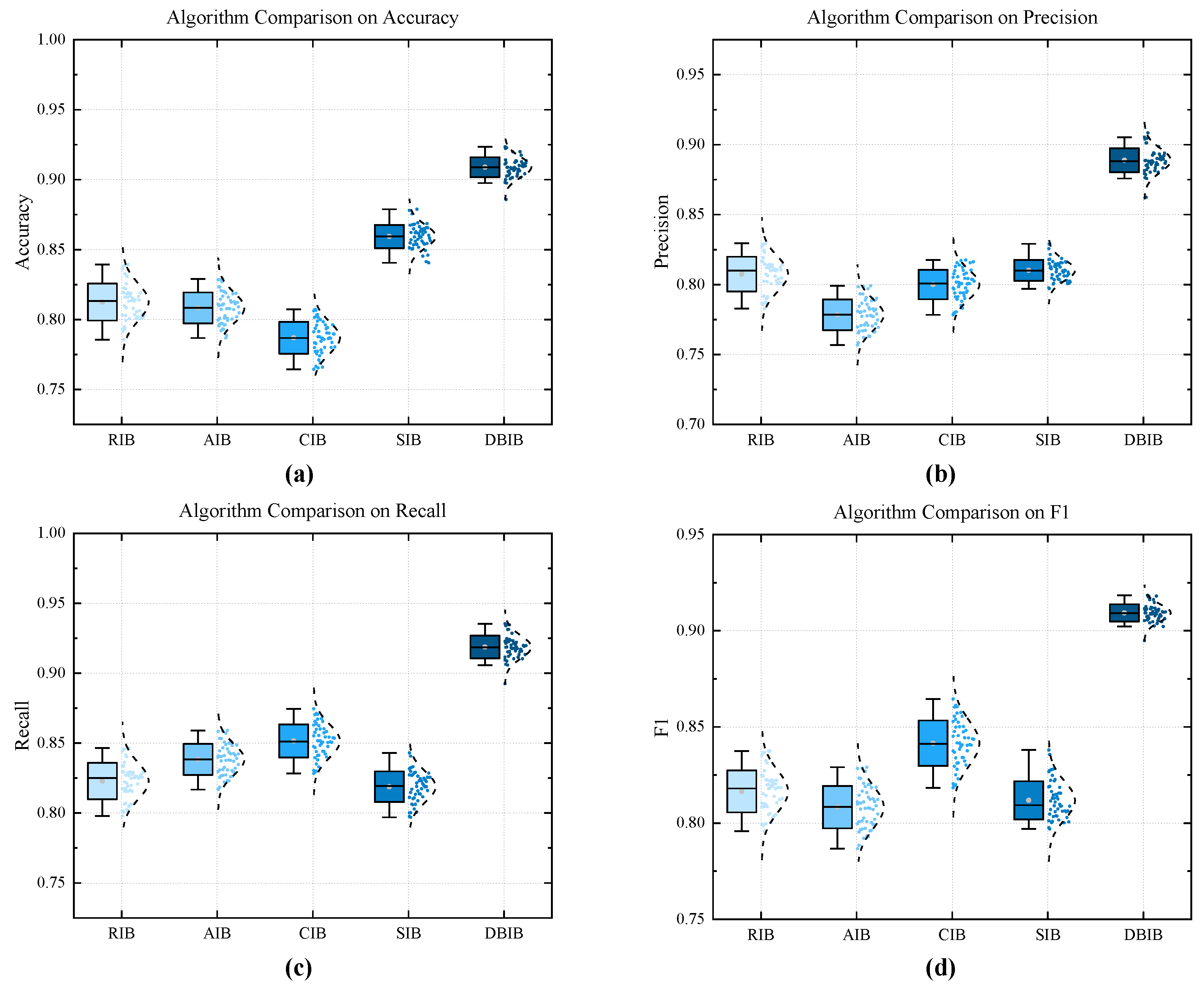
| Method | Accuracy | Precision | Recall | F1 |
|---|---|---|---|---|
| CNN-Bispectrum | 0.938 | 0.943 | 0.932 | 0.938 |
| CNN-STFT | 0.904 | 0.895 | 0.916 | 0.905 |
| CNN-CWT | 0.894 | 0.869 | 0.928 | 0.897 |
| CNN-SDP | 0.91 | 0.90 | 0.924 | 0.911 |
| CNN-Imposed Method | 0.968 | 0.964 | 0.972 | 0.968 |
Disclaimer/Publisher’s Note: The statements, opinions and data contained in all publications are solely those of the individual author(s) and contributor(s) and not of MDPI and/or the editor(s). MDPI and/or the editor(s) disclaim responsibility for any injury to people or property resulting from any ideas, methods, instructions or products referred to in the content. |
© 2025 by the authors. Licensee MDPI, Basel, Switzerland. This article is an open access article distributed under the terms and conditions of the Creative Commons Attribution (CC BY) license (https://creativecommons.org/licenses/by/4.0/).
Share and Cite
Wang, Y.; Yu, Z.; Chi, C.; Lei, B.; Pei, J.; Wang, D. Harmonic Aggregation Entropy: A Highly Discriminative Harmonic Feature Estimator for Time Series. Entropy 2025, 27, 738. https://doi.org/10.3390/e27070738
Wang Y, Yu Z, Chi C, Lei B, Pei J, Wang D. Harmonic Aggregation Entropy: A Highly Discriminative Harmonic Feature Estimator for Time Series. Entropy. 2025; 27(7):738. https://doi.org/10.3390/e27070738
Chicago/Turabian StyleWang, Ye, Zhentao Yu, Cheng Chi, Bozhong Lei, Jianxin Pei, and Dan Wang. 2025. "Harmonic Aggregation Entropy: A Highly Discriminative Harmonic Feature Estimator for Time Series" Entropy 27, no. 7: 738. https://doi.org/10.3390/e27070738
APA StyleWang, Y., Yu, Z., Chi, C., Lei, B., Pei, J., & Wang, D. (2025). Harmonic Aggregation Entropy: A Highly Discriminative Harmonic Feature Estimator for Time Series. Entropy, 27(7), 738. https://doi.org/10.3390/e27070738