Author Contributions
Conceptualization, R.S., K.Y., H.T. and M.T.; Formal Analysis, R.S.; Methodology, R.S., K.Y., H.T. and M.T.; Validation, R.S., K.Y., H.T. and M.T.; Investigation, R.S., K.Y., H.T. and M.T.; Data Curation, R.S.; Writing Original Draft Preparation, R.S.; Writing Review & Editing, R.S., K.Y., H.T. and M.T.; Visualization, R.S.; Supervision, M.T.; Project Administration, M.T.; Funding Acquisition, K.Y. and M.T. All authors have read and agreed to the published version of the manuscript.
Figure 1.
Time series of the dependent variable after pretreatment. Mean values (blue dotted line) and 1-crisis sigma (blue bandwidth) are illustrated for each period of each infected wave.
Figure 1.
Time series of the dependent variable after pretreatment. Mean values (blue dotted line) and 1-crisis sigma (blue bandwidth) are illustrated for each period of each infected wave.
Figure 2.
Behavioural pattern time series with normalization (Equation (
2)) and moving average for the last 7 days in the context of the Greater Tokyo Area (including the prefectures of Tokyo, Saitama, Chiba, Kanagawa, Ibaraki, Tochigi, Gunma, and Yamanashi).
Figure 2.
Behavioural pattern time series with normalization (Equation (
2)) and moving average for the last 7 days in the context of the Greater Tokyo Area (including the prefectures of Tokyo, Saitama, Chiba, Kanagawa, Ibaraki, Tochigi, Gunma, and Yamanashi).
Figure 3.
Flowchart of the variable selection process. The central grey area illustrates the sequential steps from raw data to preprocessing, correlation extraction, redundancy elimination, and regression accuracy evaluation. The left side indicates the corresponding sections of the paper for each step, while the right side presents the number of remaining candidate variables resulting from the variable selection process, as described in
Section 4.1 (fixed-period model).
Figure 4.
Top: Trend decomposition results () of the dependent variable time series. Bottom: One-dimensional projection of trend decomposition, where red shows an up trend, and blue shows a down trend.
Figure 4.
Top: Trend decomposition results () of the dependent variable time series. Bottom: One-dimensional projection of trend decomposition, where red shows an up trend, and blue shows a down trend.
Figure 5.
An example of applying Otsu’s method to the distribution of the absolute values of Pearson product-moment correlation coefficients for the trend time series analysed from 1 June 2020 to 31 May 2021. This figure illustrates the thresholding process (green line) that maximizes the between-class variance and the distribution (blue histogram) for data points within the range [0, 1]. The optimal threshold point (red) is identified and, as shown, tends to take a value close to the mean of the distribution (yellow line) in the absence of a clear bimodal distribution.
Figure 6.
An illustrative graph showing the relationship between the number of independent variables (horizontal axis) and the adjusted coefficient of determination (vertical axis) for the original time series of independent variables (green) and the top 1% (red), 5% (blue), and 10% (yellow) of the random walk time series.
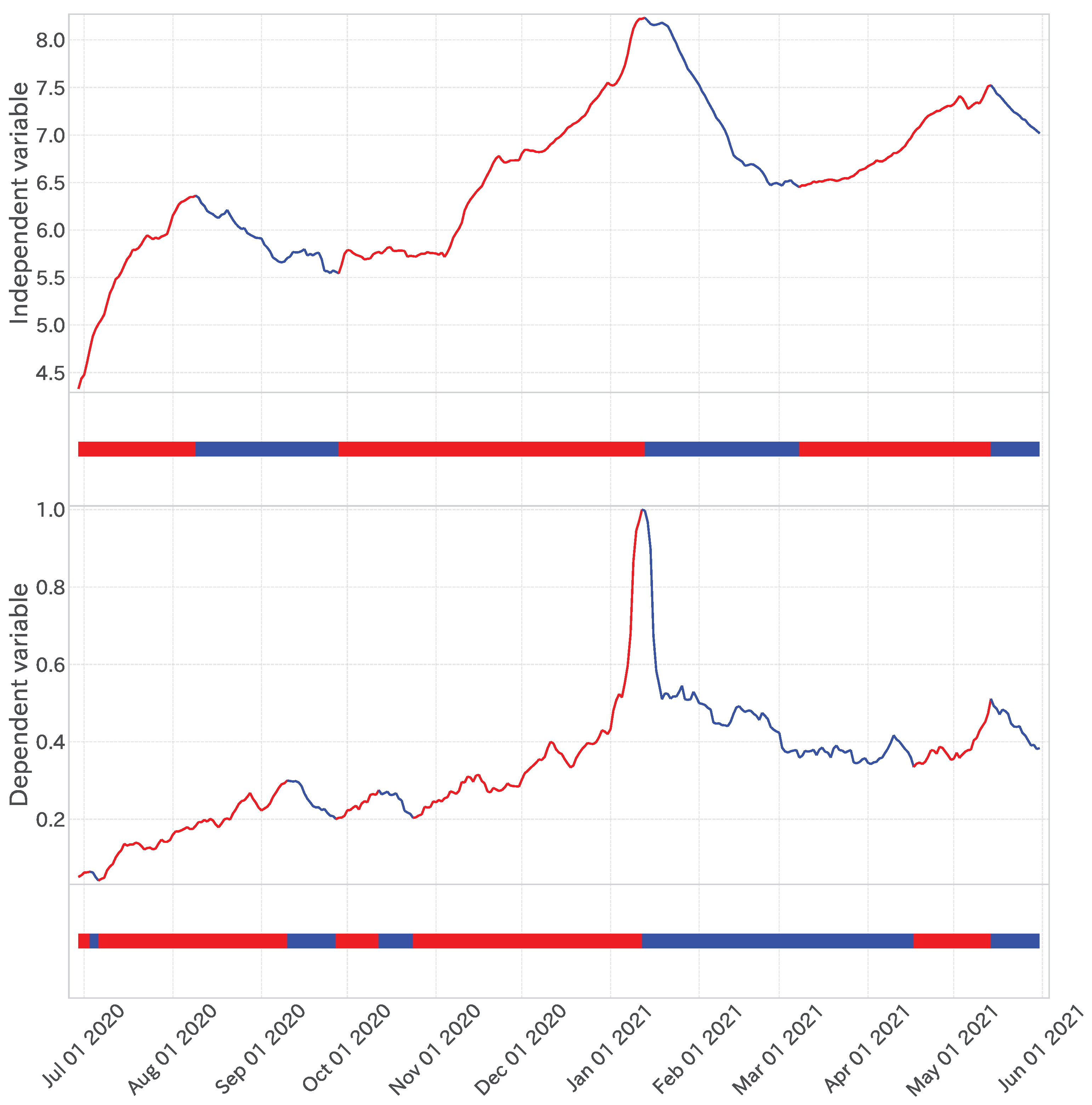
Figure 7.
The first panel depicts the time series of the dependent variable after trend decomposition; red indicates an up trend, while blue indicates a down trend. The second panel shows the result of projecting the first panel onto one dimension. The third and fourth panels similarly illustrate the time series for the explanatory variable “禍” (disaster).
Figure 8.
The blue time series represents “入院” (hospitalization), and the yellow time series represents “患者” (patients). These two series were grouped as they exhibited a Spearman’s rank correlation coefficient of 0.857. “入院” (Hospitalization) was correlated more strongly with the dependent variable, leading to the exclusion of “患者” (patients).
Figure 9.
A part of the variable selection process in the fixed-period model is depicted in this figure. It shows the relationships between the final selected variables (red nodes) and those excluded through grouping and spurious correlations (blue nodes). The numbers in the diagram represent the best lag values determined during the correlation extraction phase. Blue arrows indicate that the variable at the arrow’s base is included in the variable group pointed to by the arrow’s head. In contrast, green arrows signify that the variable at the arrow’s base was determined to have a spurious correlation with the dependent variable due to the variable at the arrow’s head.
Figure 10.
Results of the linear regression analysis for the fixed-period model. Observed values (yellow), model’s estimated values (green), and forecast interval (green band). The blue vertical lines distinguish between the learning and test periods.
Figure 10.
Results of the linear regression analysis for the fixed-period model. Observed values (yellow), model’s estimated values (green), and forecast interval (green band). The blue vertical lines distinguish between the learning and test periods.
Figure 11.
Comparison of the value obtained by multiplying the regression coefficient by the 7-day lag time series of “蔓延” (spread) (blue, right axis) with the observed values (yellow, left axis).
Figure 11.
Comparison of the value obtained by multiplying the regression coefficient by the 7-day lag time series of “蔓延” (spread) (blue, right axis) with the observed values (yellow, left axis).
Figure 12.
Histogram of errors (differences between observed and predicted values) for the fixed-period model during the test period. The upper section shows the entire test period, and the lower section shows each wave of infection.
Figure 12.
Histogram of errors (differences between observed and predicted values) for the fixed-period model during the test period. The upper section shows the entire test period, and the lower section shows each wave of infection.
Figure 13.
Results of decomposing the estimated values (top) and observed values (bottom) from the fixed-period model’s linear regression analysis into trend series. The red band represents the upward trend, and the blue band represents the downward trend. The blue vertical lines distinguish between the learning and test periods.
Figure 14.
Results of linear regression analysis for the sequential adaptive model. Observational values (yellow) and the model’s forecasting values for each infection wave (green), with forecast intervals (green band). The blue vertical lines in the figure distinguish the infection waves determined by trend decomposition.
Figure 15.
Results of the trend decomposition of the estimated values (top) and observed values (bottom) from the linear regression analysis of the sequential adaptive model. The red band represents an upward trend, and the blue band represents a downward trend. The blue vertical lines in the figure distinguish between the waves of infection determined by trend decomposition.
Figure 16.
Histogram of errors (differences between observed and predicted values) for the sequential adaptive model during the test period. The upper section shows the entire test period, the lower section shows each wave of infection.
Figure 16.
Histogram of errors (differences between observed and predicted values) for the sequential adaptive model during the test period. The upper section shows the entire test period, the lower section shows each wave of infection.
Table 1.
The p-value for the Spearman rank correlation coefficient, calculated between the dependent variable and other factors, was obtained from a sample spanning 337 days.
Table 1.
The p-value for the Spearman rank correlation coefficient, calculated between the dependent variable and other factors, was obtained from a sample spanning 337 days.
| Variable | p-Value of Spearman’s r | Lag Days | Sign of Correlation Coefficient |
|---|
| “禍” (Disaster) | | 9 | Positive |
| “株” (Strain) | | 10 | Positive |
| “蔓延” (Spread) | | 7 | Positive |
| “入院” (Hospitalization) | | 7 | Positive |
| “影響” (Impact) | | 12 | Negative |
| Move * | | 8 | Negative |
| “解消” (Cancellation) | | 28 | Negative |
Table 2.
Regression coefficients for the fixed-period model, arranged in descending order of the absolute value of Spearman’s rank correlation with the dependent variable.
Table 2.
Regression coefficients for the fixed-period model, arranged in descending order of the absolute value of Spearman’s rank correlation with the dependent variable.
| Variable | Regression Coefficient | Lag Days |
|---|
| “禍” (Disaster) | 2.48 | 9 |
| “株” (strain) | −0.09 | 10 |
| “蔓延” (Spread) | 0.95 | 7 |
| “入院” (Hospitalization) | 1.18 | 7 |
| “影響” (Impact) | −0.63 | 12 |
| Move * | 0.15 | 8 |
| “解消” (Cancellation) | −0.60 | 28 |
| Constant | 5.43 | |
Table 3.
This table compares the regression performance and trend time series classification performance of the fixed-period model and the sequential adaptive model during the test period. The observed and predicted values are broken down into trend time series. The upward trend is considered as negative results (upward) and the downward trend is considered as positive results (downward). The accuracy and Pearson Correlation remain consistent irrespective of class definition.
| Evaluation | Training Period | Test Period |
|---|
| MAE | 2.360 | 2.012 |
| Accuracy | 0.766 | 0.774 |
| Pearson Correlation | 0.499 | 0.507 |
| F1-score (Up) | 0.813 | 0.663 |
| F1-score (Down) | 0.623 | 0.830 |
Table 4.
Proportion of observed upward versus downward trends between the train and test periods.
Table 4.
Proportion of observed upward versus downward trends between the train and test periods.
| Periods | Upward | Downward |
|---|
| 2nd Wave | 42.5% | 57.5% |
| 3rd Wave | 33.4% | 66.6% |
| 4th Wave | 35.0% | 65.0% |
| 5th Wave | 60.5% | 39.5% |
| 6th Wave | 63.1% | 36.9% |
| 7th Wave | 56.3% | 43.7% |
Table 5.
This table compares the regression performance and trend time series classification performance of the fixed-period model and the sequential adaptive model during the test period. The observed and predicted values are broken down into trend time series. The upward trend is considered as negative results (upward) and the downward trend is considered as positive results (downward). The accuracy and Pearson Correlation remain consistent irrespective of class definition.
| Evaluation | Fixed-Periodmodel (Test Periods) | Sequential Adaptive Model (Test Periods) |
|---|
| MAE | 2.360 | 2.012 |
| Accuracy | 0.774 | 0.890 |
| Pearson Correlation | 0.507 | 0.775 |
| F1-score (Upward) | 0.663 | 0.864 |
| F1-score (Downward) | 0.830 | 0.908 |
Table 6.
Results of forecasting the variables of each infection wave. The parentheses show the number of lag days, and the second line in each cell displays the regression coefficient.
Table 6.
Results of forecasting the variables of each infection wave. The parentheses show the number of lag days, and the second line in each cell displays the regression coefficient.
| Prediction for 5th Wave | Prediction for 6th Wave | Prediction for 7th Wave |
|---|
| “PCR検査” (PCR Test) (7 days) | “コロナ” (COVID-19) (7 days) | “陽性” (Positive) (7 days) |
| 1.25 | 5.44 | 6.92 |
| “蔓延” (Spread) (7 days) | “懸念” (Concern ) (24 days) | Work * (7 days) |
| 0.68 | 1.22 | −2.38 |
| “突入” (Breakthrough) (11 days) | “出かける” (Go out) (9 days) | “スタート” (Start) (28 days) |
| 0.51 | −0.29 | −1.11 |
| “禁止” (Ban) (7 days) | “提供” (Provide) (18 days) | “減少” (Decrease) (28 days) |
| −0.03 | 1.78 | −4.40 |
| “拡散” (Dissemination) (7 days) | “ビール” (Bear) (19 days) | “使える” (Usable) (24 days) |
| 0.10 | −1.30 | 1.70 |
| “いける” (Can go) (12 days) | | “株” (Strain) (11 days) |
| 0.50 | | −2.65 |
| “得る” (Obtain) (7 days) | | “期間中” (During) (9 days) |
| 0.10 | | 1.70 |
Table 7.
Comparison of trend time series classification performance by accuracy. Results of the fixed-period model and the sequential adaptive model for 7-, 14-, and 21-day-ahead forecasts.
Table 7.
Comparison of trend time series classification performance by accuracy. Results of the fixed-period model and the sequential adaptive model for 7-, 14-, and 21-day-ahead forecasts.
| Test Period (Accuracy) | 7 Day | 14 Day | 21 Day |
|---|
| Fixed-period model | 0.774 | 0.705 | 0.657 |
| Sequential adaptive model | 0.890 | 0.784 | 0.752 |


