
Physics-Informed Neural Networks with Unknown Partial Differential Equations: An Application in Multivariate Time Series


Abstract
1. Introduction
2. Differential Equations
3. Methods of PDE Construction
3.1. Sparse Identification of Nonlinear Dynamics (SINDy)
3.2. Least Absolute Shrinkage and Selection Operator (LASSO)
3.3. Bayesian Least Absolute Shrinkage and Selection Operator (B-LASSO)
3.4. Symbolic Regression (SR)
3.5. Convolutional Neural Network (CNN)
3.6. Temporal Convolutional Network (TCN)
4. Physics-Informed Neural Network (PINN)
5. Bayesian Computations
5.1. Physics-Informed Bayesian Linear Regression (PI-BLR)
5.2. Bayesian Physics-Informed Neural Network (B-PINN)
6. A Real-World MTS Dataset
- Elapsed Time : The time that has passed since the beginning of the data collection period, measured in hours. This variable enables us to analyze trends and patterns in energy consumption over time, facilitating time-based analyses and comparisons.
- Global Active Power and : The total active power consumed by the household, averaged over each minute (in kilowatts).
- Global Reactive Power and : The total reactive power consumed by the household, averaged over each minute (in kilowatts).
- Voltage and : The minute-averaged voltage (in volts).
- Global Intensity: The minute-averaged current intensity (in amperes). This variable is a linear function of Global Active Power, so we omit it from the dataset.
- Sub-metering1 and : Energy consumption (in watt-hours) corresponding to the kitchen, primarily attributed to appliances such as a dishwasher, oven, and microwave.
- Sub-metering2 and : Energy consumption (in watt-hours) corresponding to the laundry room, including a washing machine, tumble-drier, refrigerator, and lighting.
- Sub-metering3 and : Energy consumption (in watt-hours) corresponding to an electric water heater and air conditioner.
- Check the correlations between variables and remove those with linear relationships.
- Use interpolation methods like first-order spline to fill in missing data gaps.
- Normalize the data to facilitate capturing complex relationships between variables.
- Divide the data into two portions: approximately for the PDE construction phase and for the prediction phase using data-driven PDEs. Additionally, split each segment into training, validation, and testing sets.
- Apply the PDE construction methods outlined in Section 3:
- Train the physics-informed network using of the remaining samples, along with the data-driven PDEs.
- Use the previous T samples to predict a point in the future. Then, iteratively apply the same process, using the latest predicted values as inputs to generate subsequent future points. Continue this hierarchical prediction until you reach the desired number of future predictions.
- Evaluate the predictions using metrics such as MSE.
7. Conclusions
Author Contributions
Funding
Data Availability Statement
Conflicts of Interest
Appendix A. SINDy Algorithm
- Prepare the system data for inputs and for outputs. Here, n represents the number of samples, d denotes the number of input features, and p indicates the number of target variables. Note that the input contains both dynamic and state variables, while the output consists of the state variables of , excluding the dynamic variables. In some applications, there might be only one dynamic variable (e.g., elapsed time t), which leads to the relationship . For clarification, consider the following example:where is the only dynamic variable.When dealing with MTS, it is important to account for time steps when preparing the output variables. The output variable should be shifted by T samples from the input corresponding to the state variables, which is known as the lag operator in MTS contexts. This means that the first T samples of the state variables in must be removed to construct the outputs. The larger the value of T, the more accurate the predictions become, but this also requires more computation. To simplify notation, assume the number of samples in both and is equal to n.
- Calculate the necessary derivatives of the output variables with respect to the dynamic variables:where for is defined:where is the number of dynamic variables. In this definition, can be replaced by d to take the derivatives with respect to all inputs if desired. This may involve numerical differentiation techniques to estimate the derivatives from the collected data. In this context, represents the total number of dynamic variables.
- Create a library of potential basic functions for the state variables , including polynomial terms, interactions between variables, trigonometric functions, and other relevant functions that may describe the dynamics of the system. This step is crucial, as it lays the foundation for accurately identifying the underlying equations that govern the system’s behavior. For more complex models, one might also incorporate the derivatives of into the potential function, resulting in , where .
- Formulate the sparse regression problem , where is the coefficient vector to estimate, and ⊙ is the Hadamard product.
- Regularize the coefficient vector. This step helps prevent the coefficients from becoming excessively large and promotes sparsity by shrinking some coefficients to zero. Regularization adds a penalty term to the loss function that encourages sparsity. Refine the coefficient by minimizingwhere and are the and norms, respectively.
- Select the active terms from the regression results that have non-zero coefficients.
- Assemble the identified terms into a mathematical model, typically in the form of a PDE.
- Validate the constructed model against the original data and select the equations that accurately describe the data.
Appendix B. LASSO Algorithm
- Perform same as the SINDy Algorithm to define . In this algorithm, the derivatives are obtained not only with respect to the dynamic variables, but also for other features of the input set.
- Formulate the LASSO regression model as
- Choose a range of values to test (e.g., , , 1, 10, 100).
- Implement k-fold cross-validation by splitting the data into k subsets. Use each subset as the validation set and the remaining subsets as the training set.
- Fit the LASSO model to the training set using the current .
- Calculate the MSE or MAE on the validation set and average them across all k folds for each .
- Using the optimal found from cross-validation, fit the LASSO model to the entire dataset X and Y to find . For simplicity, one can skip Steps 3 and 4 and use a predetermined value for .
- Formulate the constructed function as a PDE based on the non-zero coefficients.
- Validate the constructed PDE against a separate dataset to ensure its predictive capability.
Appendix C. B-LASSO Algorithm
- Follow Steps 1 to 3 in the SINDy Algorithm to prepare the data and define the design matrix.
- Formulate the B-LASSO model as follows:where represents the regression coefficients of the model, denotes the positive real regularization parameters, and is the model noise factor. The hyperparameters , , , , and can be approximated based on data. The symbols , , , and represent the Normal, Laplace, Gamma, and Half-Cauchy distributions, respectively. For simplicity, can be identity function.
- Estimate the posterior distribution using a sampling method such as MCMC. The posterior distribution of the parameters , , and given the data and is expressed as
- Approximate the coefficients using the posterior distribution samples:where represents the ith sample of from the jth chain, N is the number of draws per chain, and M is the number of chains. In this context, the highest density interval of the coefficients can be used to measure uncertainty for a specified confidence level, such as . The HDI is a Bayesian credible interval that contains the most probable values of the posterior distribution.
- Construct PDEs based on the non-zero coefficients in the form .
- Evaluate the constructed PDEs using unseen data and select the equations that demonstrate high accuracy.
Appendix D. SR Algorithm
- Prepare the relevant input features and target features .
- Compute the derivative matrix of the output variables with respect to the input variables.
- Utilize a SR package, such as gplearn (a Python library for SR based on genetic programming, for example, version ), to approximate the relationship between the derivatives and the target variables.
- Fit a symbolic regressor to the training data to approximate the relationship:The symbolic regressor searches for a mathematical expression that minimizes the error:
- Construct the best performing equation from the symbolic regressor . For example, one PDE may have the form:where is the first target feature, is the first input feature, and represents all input features except the first one.
- Evaluate the constructed PDEs and select those with high accuracy.
Appendix E. CNN Algorithm
- Provide the input features and the target variables , where T is the number of time steps, known as lags and explained in Appendix A. For example, means that 10 previous time steps are used to predict the value at time .
- Apply one-dimensional convolutional layers with filters to the lth layer, where m is the kernel size. The output of the lth convolutional layer iswhere * denotes the convolution operation, is the output of the previous layer, is the bias term, and ReLU is the activation function.
- Use max-pooling to reduce the dimensionality of the feature maps:
- Flatten the output of the final convolutional layer and pass it through a fully connected layer to produce the predicted outputs :where and are the weights and biases of the last layer and · denotes matrix multiplication.
- Train the model using the MSE loss function. To obtain accurate derivatives, it is essential to have a well-trained network, as this ensures the reliability of the derivatives produced afterward.
- Compute the derivatives of the predicted outputs with respect to the input features using automatic differentiation:
- Organize the derivatives into a matrix , where each entry represents the derivative of the jth output variable with respect to the kth input feature at time step t for the ith sample:
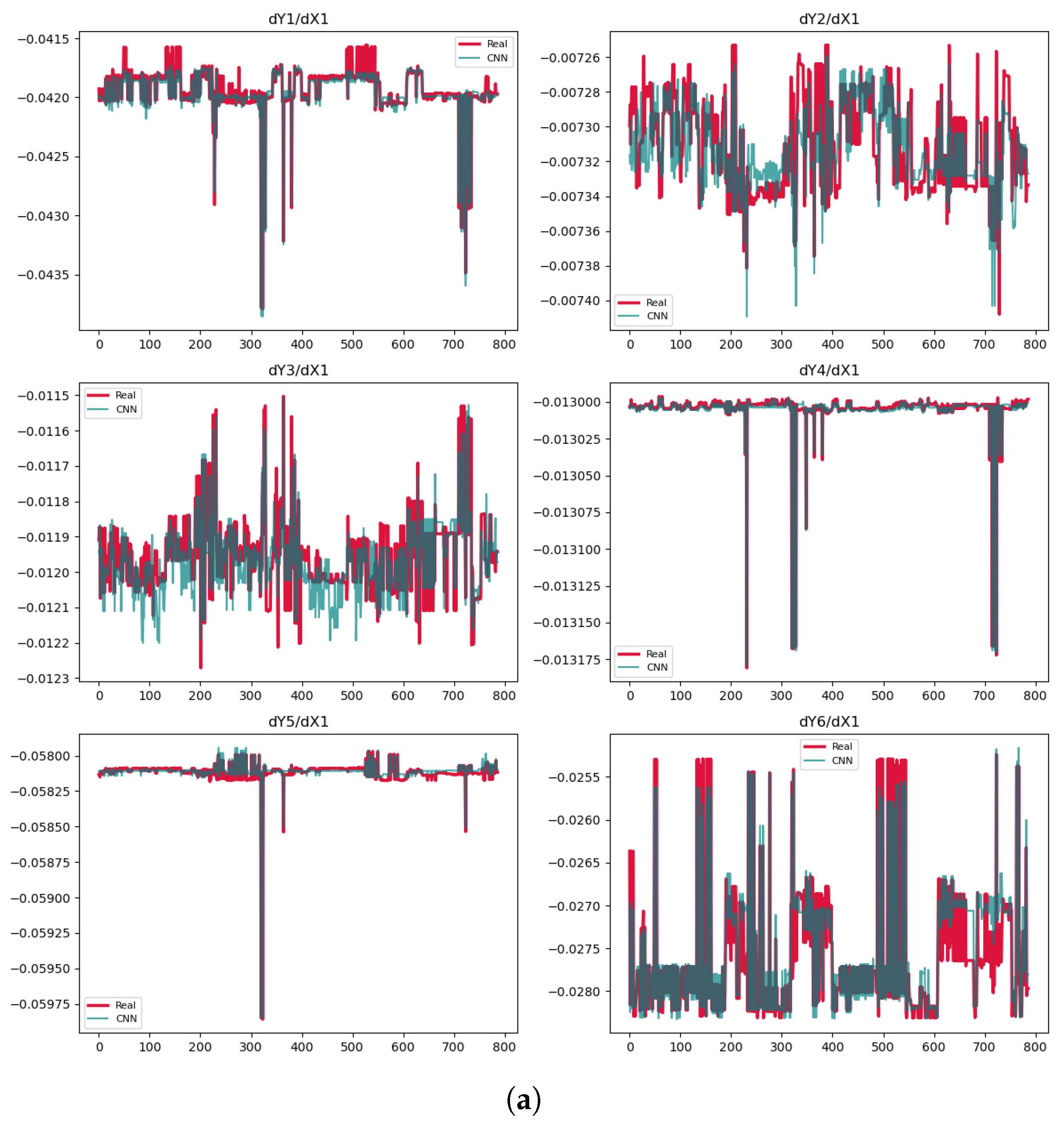
- Perform a correlation analysis between the derivatives and the target variables to identify the most significant terms in the PDEs. Compute the correlation matrix to quantify the relationships.
- Select the derivatives with the highest correlation (e.g., correlation greater than ) to the target variables. These derivatives are considered candidate terms for the PDEs. For example, to construct a PDE for a specific output feature with respect to a specific input feature, such as , we select the most relevant derivatives and state variables associated with the desired derivative.
- Approximate the relationship between the significant derivatives and the target variables using a polynomial regression model. The resulting polynomial equation represents the constructed PDE:where represents polynomial features of degree q constructed from the significant derivatives and state variables.
- Evaluate the accuracy of the constructed PDEs and select those with the highest predictive performance.
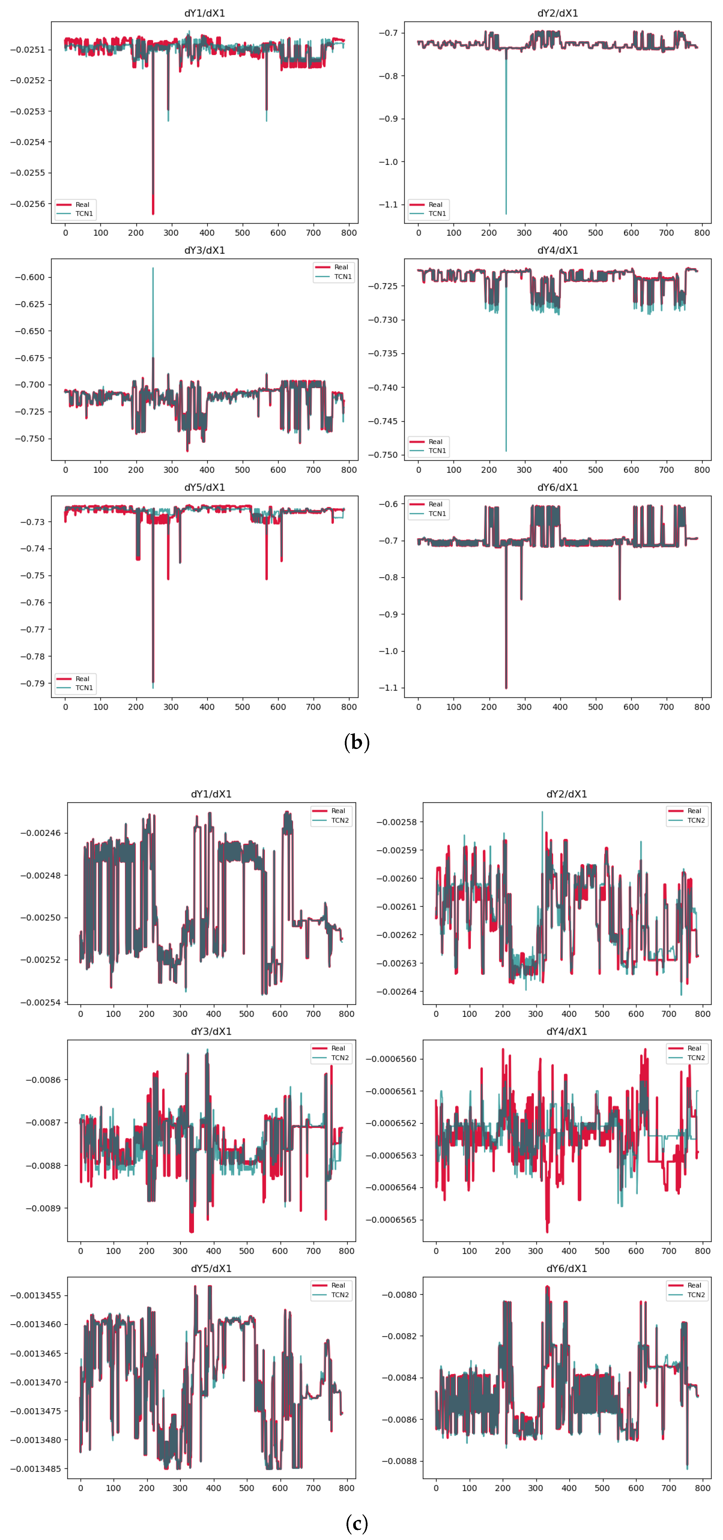
Appendix F. TCN Algorithm
- Follow Step 1 of the CNN Algorithm.
- Apply a TCN to the input data. The TCN consists of multiple dilated convolutional layers with causal padding to preserve the temporal order of the data. The output of the lth dilated convolutional layer is given bywhere denotes the causal convolution operation with a dilation rate that increases exponentially with each layer. To ensure that the model does not utilize future information for predictions, causal padding is applied. For a kernel of size m and a dilation rate , the input is padded with zeros on the left side.
- Add residual connections to improve gradient flow and stabilize training. For the lth layer, the residual connection is computed aswhere and are the residual weights and bias. The final output of the layer is
- Perform Steps 4 to 11 of the CNN Algorithm.
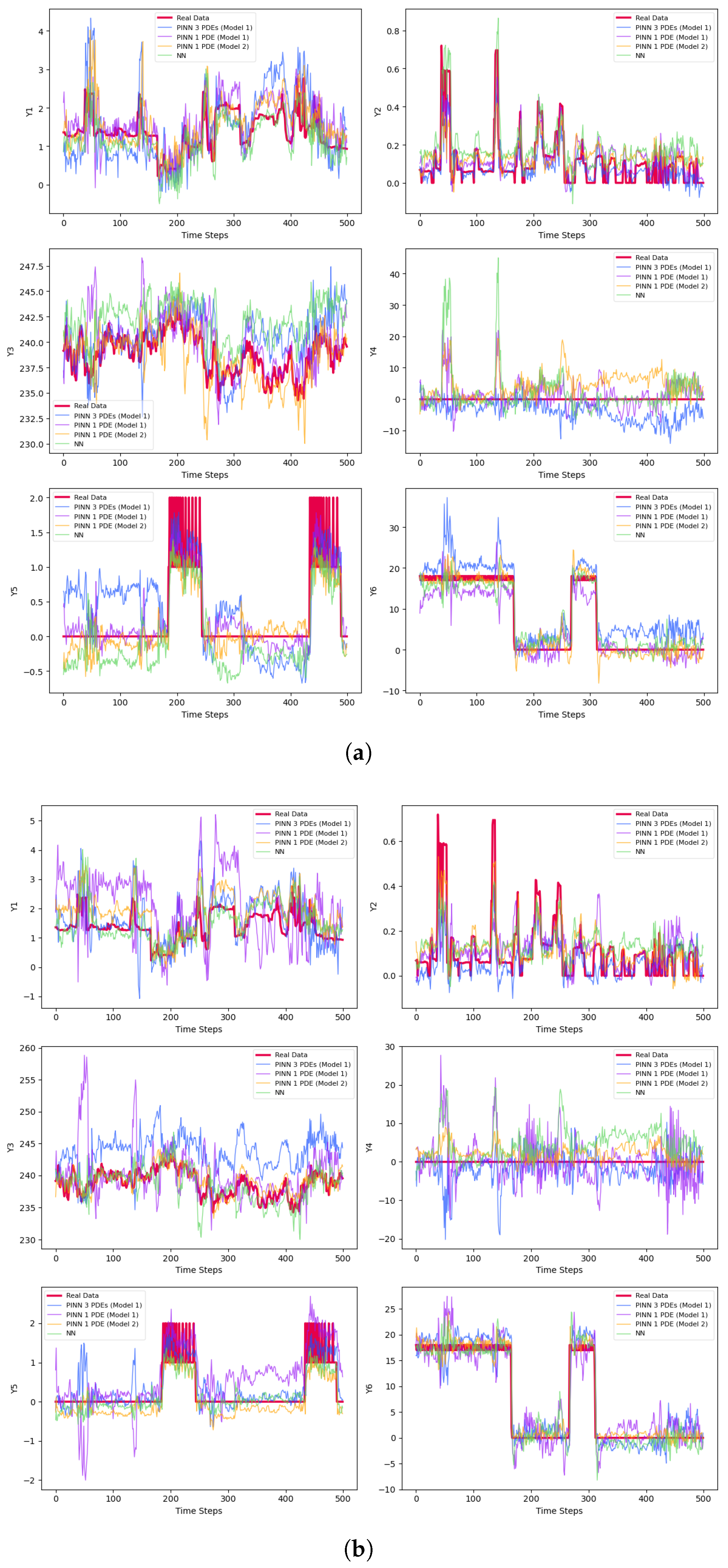
Appendix G. PINN Algorithm
- Prepare a new dataset of inputs and outputs , similar to Step 1 in the SINDy Algorithm.
- Create a NN architecture aligned with the number of inputs and outputs according to the data.
- Define the physical loss function based on the constructed PDEs. For example, if a PDE is constructed aswhere is a non-linear function, , and , then the loss function is defined by the MSE:where is a vector of zeros and ones. The values of indicate whether the corresponding derivative equations are included in the loss function based on the PDE construction. If , then contributes to the loss function; conversely, indicates that no equation is defined for , and it is excluded from the loss.
- Determine the data loss function :
- Combine the physics loss and data loss into a total loss function :Although MSE is used in this algorithm, other loss functions can also be applied.
- Use the Adam optimizer or any other suitable optimizer to minimize with respect to the network weights and biases.
- Train the model for a fixed number of epochs.
- Evaluate the trained model on the validation and test sets using the total loss function. If necessary, refine or tune the hyperparameters to achieve better results.
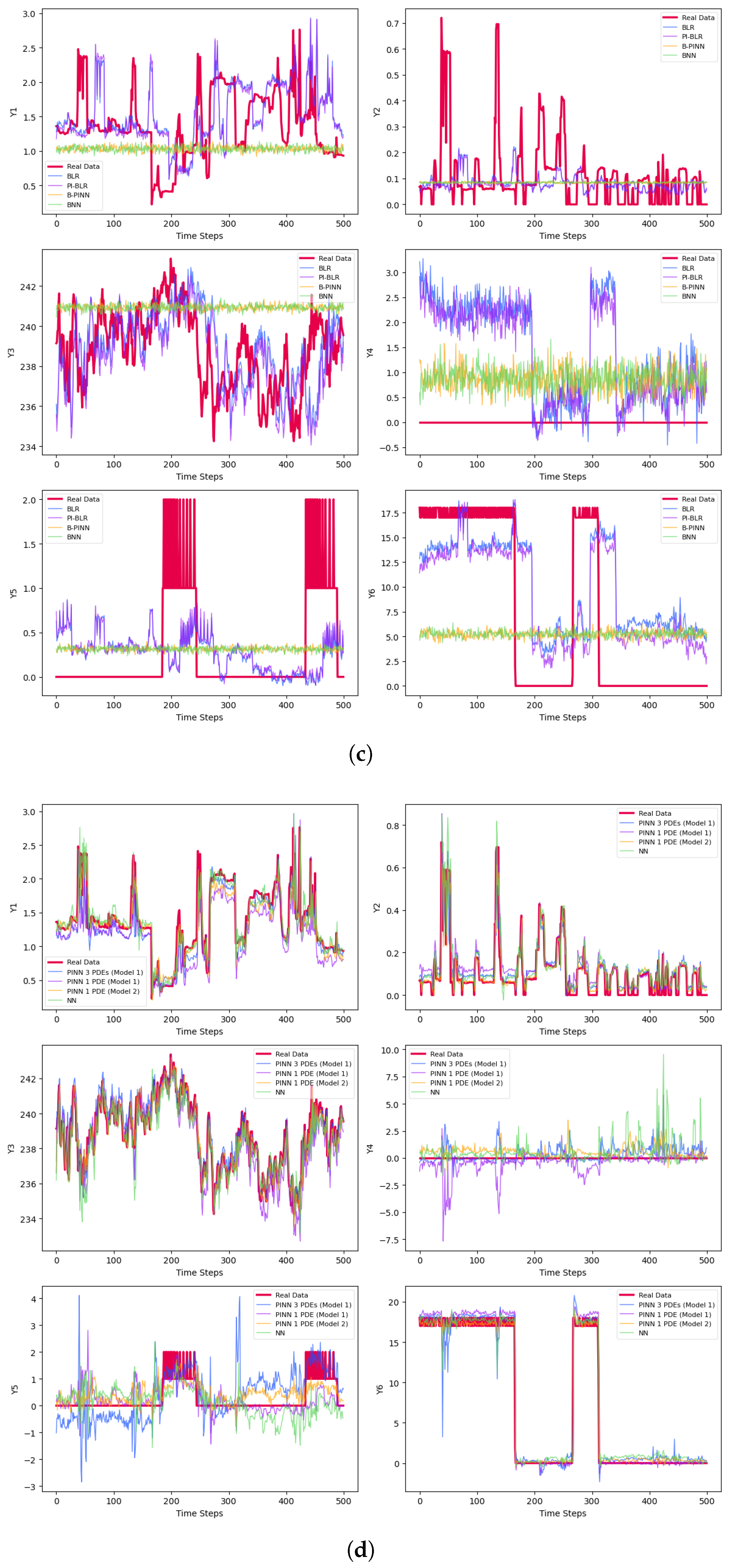
Appendix H. PI-BLR Algorithm
- Prepare the input variable and the output target , similar to the SINDy Algorithm.
- Define the priors and the Normal likelihood for the observed outputs:where , , and are hyperparameters. The term is included to enhance sampling efficiency, while represents the regression coefficients with a non-centered parameterization for stable sampling. The scale parameters enforce sparsity through Gamma priors.
- Specify the desired PDEs as in Step 3 of the PINN Algorithm.
- Construct the posterior distribution of , , and given the data and :
- Set the PDEs to zero:Note that does not need to be defined for all j and i. For undefined cases, assume it to be zero. For simplicity, assume there are PDEs, which can be denoted as . The derivatives are inherently dependent on the coefficients , although this dependence may not be explicitly clear in the preceding formula. This relationship is derived based on the model established in Step 2. The PDE residuals act as soft constraints, weighted by , which can be interpreted as assuming the PDE residuals follow a zero-mean Normal distribution:The logarithmic term for the PDEs is given byHere, serves as a quadratic penalty, equivalent to a Normal prior on the PDE residuals.
- Rewrite the posterior distribution to incorporate the physics-based potential term, penalizing deviations from domain-specific PDEs:
- Find the maximum a posteriori estimation to initialize the parameters:where , , and are the initialization parameter estimations.
- Sample from the full posterior using the No-U-Turn Sampler (NUTS) and specify appropriate values for the number of chains, tuning steps, number of returned samples, target acceptance rate, and maximum tree depth. It is worth mentioning that tuning steps, also known as burn-in, refer to the number of initial samples to discard before collecting the desired number of samples from each chain.
- Evaluate the model on an unseen dataset and adjust the hyperparameters as necessary.
Appendix I. B-PINN Algorithm
- Start by following Step 1 of the SINDy Algorithm to load the input and output datasets.
- Define the initial layer and subsequent layers using a non-centered parameterization of weights:where c is a small scalar, such as , to ensure the weights are non-centered, and L represents the total number of layers. All weights and biases are assumed to follow distributions and , respectively, with typical values being and . The hyperbolic tangent function is omitted in the last layer for regression tasks.
- Assign a Half-Normal prior to the observational noise, represented as , where denotes the Half-Normal distribution. This prior, being lighter-tailed compared to Half-Cauchy, enhances identifiability in high-dimensional B-PINNs by penalizing large noise values.
- Construct the likelihood function based on the prediction :
- Formulate the PDEs as outlined in Steps 3 and 5 of the PI-BLR Algorithm.
- Define the hierarchical Bayesian inference using either the PDEs or by omitting their current term to formulate a BNN:
- Use Automatic Differentiation Variational Inference (ADVI) to approximate initial points for the parameters. ADVI is a type of variational inference aimed at approximating the true posterior distribution by a simpler, parameterized distribution, achieved by minimizing the Kullback–Leibler divergence between the two distributions.
- Sample from the approximated posterior distribution using NUTS with the hyperparameters defined in Step 8 of the PI-BLR Algorithm.
- Evaluate the trained model to determine its reliability.
References
- Raissi, M.; Perdikaris, P.; Karniadakis, G.E. Physics-informed neural networks: A deep learning framework for solving forward and inverse problems involving nonlinear partial differential equations. J. Comput. Phys. 2019, 378, 686–707. [Google Scholar]
- Bararnia, H.; Esmaeilpour, M. On the application of physics informed neural networks (PINN) to solve boundary layer thermal-fluid problems. Int. Commun. Heat Mass Transf. 2022, 132, 105890. [Google Scholar]
- Hu, H.; Qi, L.; Chao, X. Physics-informed neural networks (PINN) for computational solid mechanics: Numerical frameworks and applications. Thin-Walled Struct. 2024, 205, 112495. [Google Scholar]
- Wang, D.; Jiang, X.; Song, Y.; Fu, M.; Zhang, Z.; Chen, X.; Zhang, M. Applications of physics-informed neural network for optical fiber communications. IEEE Commun. Mag. 2022, 60, 32–37. [Google Scholar]
- Mohammad-Djafari, A.; Chu, N.; Niven, R.K. Physics informed neural networks for inverse problems and dynamical system identification. In Proceedings of the 24th Australasian Fluid Mechanics Conference, Canberra, Australia, 1–5 December 2024. [Google Scholar]
- Liang, G.; Tiwari, P.; Nowaczyk, S.; Byttner, S. Higher-order spatio-temporal physics-incorporated graph neural network for multivariate time series imputation. In Proceedings of the 33rd ACM International Conference on Information and Knowledge Management, Boise, ID, USA, 21–25 October 2024; pp. 1356–1366. [Google Scholar]
- Nayek, R.; Fuentes, R.; Worden, K.; Cross, E.J. On spike-and-slab priors for Bayesian equation discovery of nonlinear dynamical systems via sparse linear regression. Mech. Syst. Signal Process. 2021, 161, 107986. [Google Scholar]
- Tang, J.; Fu, C.; Mi, C.; Liu, H. An interval sequential linear programming for nonlinear robust optimization problems. Appl. Math. Model. 2022, 107, 256–274. [Google Scholar]
- Tang, J.; Li, X.; Fu, C.; Liu, H.; Cao, L.; Mi, C.; Yu, J.; Yao, Q. A possibility-based solution framework for interval uncertainty-based design optimization. Appl. Math. Model. 2024, 125, 649–667. [Google Scholar]
- Niven, R.K.; Cordier, L.; Mohammad-Djafari, A.; Abel, M.; Quade, M. Dynamical system identification, model selection, and model uncertainty quantification by bayesian inference. Chaos Interdiscip. J. Nonlinear Sci. 2024, 34, 083140. [Google Scholar]
- Zwillinger, D.; Dobrushkin, V. Handbook of Differential Equations; Chapman and Hall/CRC: Boston, MA, USA, 2021. [Google Scholar]
- Peitz, S.; Stenner, J.; Chidananda, V.; Wallscheid, O.; Brunton, S.L.; Taira, K. Distributed control of partial differential equations using convolutional reinforcement learning. Phys. D Nonlinear Phenom. 2024, 461, 134096. [Google Scholar]
- Brunton, S.L.; Proctor, J.L.; Kutz, J.N. Discovering governing equations from data by sparse identification of nonlinear dynamical systems. Proc. Natl. Acad. Sci. USA 2016, 113, 3932–3937. [Google Scholar]
- Fasel, U.; Kutz, J.N.; Brunton, B.W.; Brunton, S.L. Ensemble-SINDy: Robust sparse model discovery in the low-data, high-noise limit, with active learning and control. Proc. R. Soc. A 2022, 478, 20210904. [Google Scholar]
- Schmid, A.C.; Doostan, A.; Pourahmadian, F. Ensemble WSINDy for data driven discovery of governing equations from laser-based full-field measurements. arXiv 2024, arXiv:2409.20510. [Google Scholar]
- Tibshirani, R. Regression shrinkage and selection via the LASSO. J. R. Stat. Soc. Ser. B Stat. Methodol. 1996, 58, 267–288. [Google Scholar]
- Zhan, Y.; Guo, Z.; Yan, B.; Chen, K.; Chang, Z.; Babovic, V.; Zheng, C. Physics-informed identification of PDEs with LASSO regression, examples of groundwater-related equations. J. Hydrol. 2024, 638, 131504. [Google Scholar]
- Ma, M.; Fu, L.; Guo, X.; Zhai, Z. Incorporating LASSO regression to physics-informed neural network for inverse PDE problem. CMES-Comput. Model. Eng. Sci. 2024, 141, 385–399. [Google Scholar]
- Park, T.; Casella, G. The Bayesian LASSO. J. Am. Stat. Assoc. 2008, 103, 681–686. [Google Scholar]
- Chen, J.; Guo, Z.; Zhang, L.; Pan, J. A partially confirmatory approach to scale development with the Bayesian LASSO. Psychol. Methods 2021, 26, 210. [Google Scholar]
- Changdar, S.; Bhaumik, B.; Sadhukhan, N.; Pandey, S.; Mukhopadhyay, S.; De, S.; Bakalis, S. Integrating symbolic regression with physics-informed neural networks for simulating nonlinear wave dynamics in arterial blood flow. Phys. Fluids 2024, 36, 121924. [Google Scholar]
- Liu, Y.Y.; Shen, J.X.; Yang, P.P.; Yang, X.W. A CNN-PINN-DRL driven method for shape optimization of airfoils. Eng. Appl. Comput. Fluid Mech. 2025, 19, 2445144. [Google Scholar]
- Perumal, V.; Abueidda, D.; Koric, S.; Kontsos, A. Temporal convolutional networks for data-driven thermal modeling of directed energy deposition. J. Manuf. Process. 2023, 85, 405–416. [Google Scholar]
- Fraza, C.J.; Dinga, R.; Beckmann, C.F.; Marquand, A.F. Warped Bayesian linear regression for normative modelling of big data. NeuroImage 2021, 245, 118715. [Google Scholar]
- Gholipourshahraki, T.; Bai, Z.; Shrestha, M.; Hjelholt, A.; Hu, S.; Kjolby, M.; Rohde, P.D.; Sørensen, P. Evaluation of Bayesian linear regression models for gene set prioritization in complex diseases. PLoS Genet. 2024, 20, e1011463. [Google Scholar]
- Yang, L.; Meng, X.; Karniadakis, G.E. B-PINNs: Bayesian physics-informed neural networks for forward and inverse PDE problems with noisy data. J. Comput. Phys. 2021, 425, 109913. [Google Scholar]
- Mohammad-Djafari, A. Bayesian physics informed neural networks for linear inverse problems. arXiv 2025, arXiv:2502.13827. [Google Scholar]
- Repository, U.M.L. Household Electric Power Consumption. 2020. Available online: https://www.kaggle.com/datasets/uciml/electric-power-consumption-data-set (accessed on 3 March 2023).


| Phase | Methods | Variable | MSE | MAE | |
|---|---|---|---|---|---|
| PDE constructions 1,958,991 training 19,000 validation 788 testing | CNN | ||||
| TCN Model 1 | |||||
| TCN Model 2 | |||||
| Phase | Methods | Variable | MSE | MAE | |
|---|---|---|---|---|---|
| PDE constructions 1,958,991 training 19,000 validation 788 testing | SINDy | ||||
| LASSO | |||||
| B-LASSO | |||||
| SR | |||||
| CNN | |||||
| TCN Model 1 vs. Model 2 | |||||
| Phase | Methods | Variable | MSE | MAE | |
|---|---|---|---|---|---|
| Predictions small samples | NN 50 Epochs | ||||
| NN Early-Stop | |||||
| PINN 3 PDEs Model 1 50 Epochs | |||||
| PINN 3 PDEs Model 1 Early-Stop | |||||
| PINN 1 PDE Model 1 50 Epochs | |||||
| PINN 1 PDE Model 1 Early-Stop | |||||
| Predictions small samples | PINN 1 PDE Model 2 50 Epochs | ||||
| PINN 1 PDE Model 2 Early-Stop | |||||
| BLR 230 samples 200 tuning 1 chain | |||||
| PI-BLR 3 PDEs Model 1 230 samples 200 tuning 1 chain | |||||
| BNN 10 neurons 2 hidden layers 230 samples 200 tuning 1 chain | |||||
| B-PINN 3 PDEs, Model 1 10 neurons 2 hidden layers 230 samples 200 tuning, 1 chain | |||||
| Predictions medium samples | NN 50 Epochs | ||||
| NN Early-Stop | |||||
| Predictions medium samples | PINN 3 PDEs model 1 50 Epochs | ||||
| PINN 3 PDEs Model 1 Early-Stop | |||||
| PINN 1 PDE Model 1 50 Epochs | |||||
| PINN 1 PDE Model 1 Early-Stop | |||||
| Predictions medium samples | PINN 1 PDE Model 2 50 Epochs | ||||
| PINN 1 PDE Model 2 Early-Stop | |||||
| BLR 230 samples 200 tuning 1 chain | |||||
| PI-BLR 3 PDEs Model 1 230 samples 200 tuning 1 chain | |||||
| Predictions medium samples | BNN 10 neurons 2 hidden layers 230 samples 200 tuning 1 chain | ||||
| B-PINN 3 PDEs, Model 1 10 neurons 2 hidden layers 230 samples 200 tuning, 1 chain | |||||
| Predictions large samples | NN 50 Epochs | ||||
| NN Early-Stop | |||||
| PINN 3 PDEs Model 1 50 Epochs | |||||
| PINN 3 PDEs Model 1 Early-Stop | |||||
| PINN 1 PDE Model 1 50 Epochs | |||||
| PINN 1 PDE Model 1 Early-Stop | |||||
| Predictions large samples | PINN 1 PDE Model 2 50 Epochs | ||||
| PINN 1 PDE Model 2 Early-Stop | |||||
| BLR 230 samples 200 tuning 1 chain | |||||
| PI-BLR 3 PDEs Model 1 230 samples 200 tuning 1 chain | |||||
| BNN 10 neurons 2 hidden layers 230 samples 200 tuning 1 chain | |||||
| B-PINN 3 PDEs, Model 1 10 neurons 2 hidden layers 230 samples 200 tuning, 1 chain | |||||
Disclaimer/Publisher’s Note: The statements, opinions and data contained in all publications are solely those of the individual author(s) and contributor(s) and not of MDPI and/or the editor(s). MDPI and/or the editor(s) disclaim responsibility for any injury to people or property resulting from any ideas, methods, instructions or products referred to in the content. |
© 2025 by the authors. Licensee MDPI, Basel, Switzerland. This article is an open access article distributed under the terms and conditions of the Creative Commons Attribution (CC BY) license (https://creativecommons.org/licenses/by/4.0/).
Share and Cite
Mortezanejad, S.A.F.; Wang, R.; Mohammad-Djafari, A. Physics-Informed Neural Networks with Unknown Partial Differential Equations: An Application in Multivariate Time Series. Entropy 2025, 27, 682. https://doi.org/10.3390/e27070682
Mortezanejad SAF, Wang R, Mohammad-Djafari A. Physics-Informed Neural Networks with Unknown Partial Differential Equations: An Application in Multivariate Time Series. Entropy. 2025; 27(7):682. https://doi.org/10.3390/e27070682
Chicago/Turabian StyleMortezanejad, Seyedeh Azadeh Fallah, Ruochen Wang, and Ali Mohammad-Djafari. 2025. "Physics-Informed Neural Networks with Unknown Partial Differential Equations: An Application in Multivariate Time Series" Entropy 27, no. 7: 682. https://doi.org/10.3390/e27070682
APA StyleMortezanejad, S. A. F., Wang, R., & Mohammad-Djafari, A. (2025). Physics-Informed Neural Networks with Unknown Partial Differential Equations: An Application in Multivariate Time Series. Entropy, 27(7), 682. https://doi.org/10.3390/e27070682