

Reputation in the Iterated Prisoner’s Dilemma: A Simple, Analytically Solvable Agents’ Model


Abstract
1. Introduction
2. Model
- The first agent is chosen randomly with uniform probability. Thus, the probability of selecting a given agent is , and it does not depend on the reputation of the agent.
- The second agent is selected in a two-stage process. Firstly, agents are randomly selected according to a uniform probability (the probability of selecting a given agent is ). Then, from this group of n agents, one with the highest reputation is taken.
3. Results
3.1. Case 1:
3.2. Case 2:
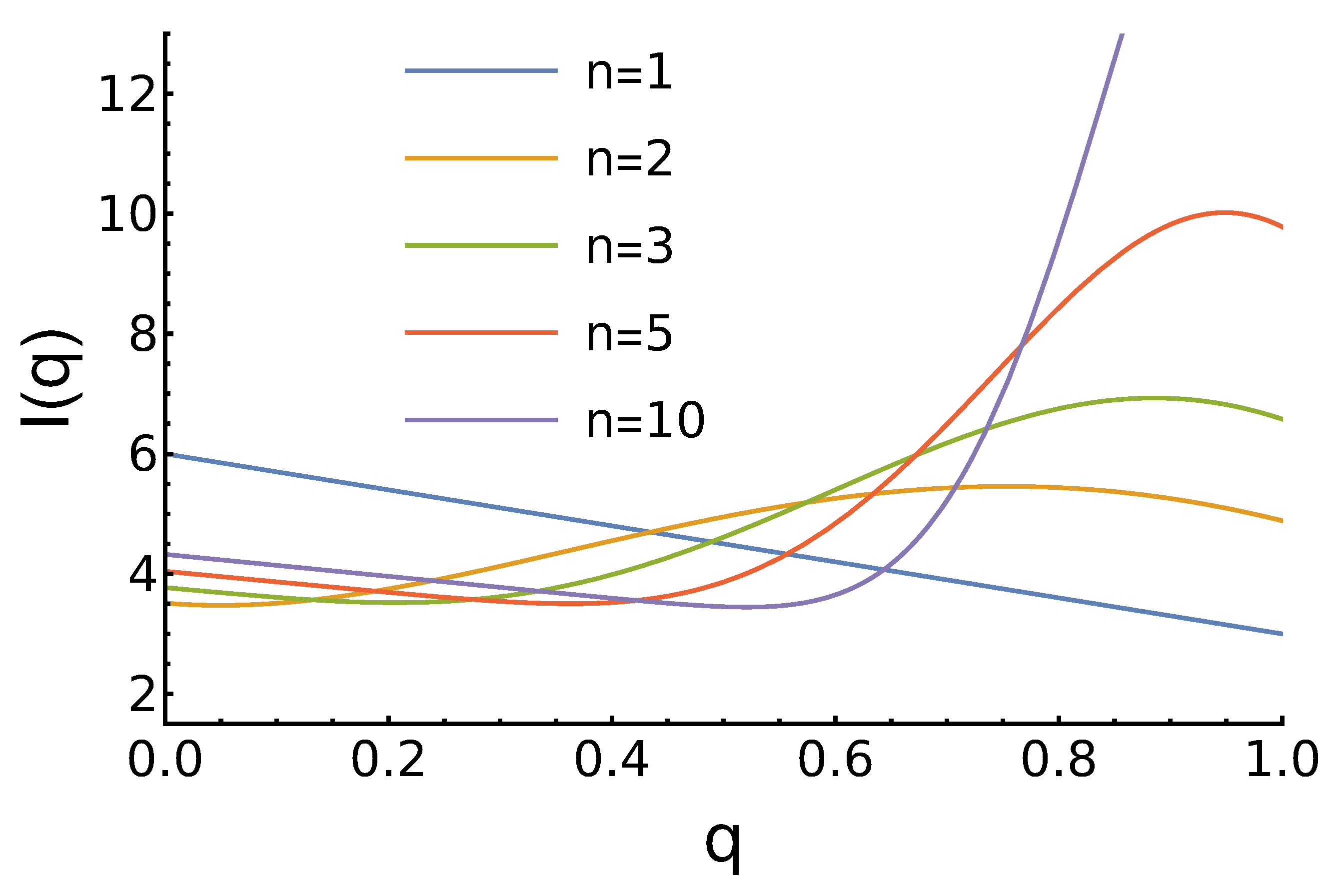
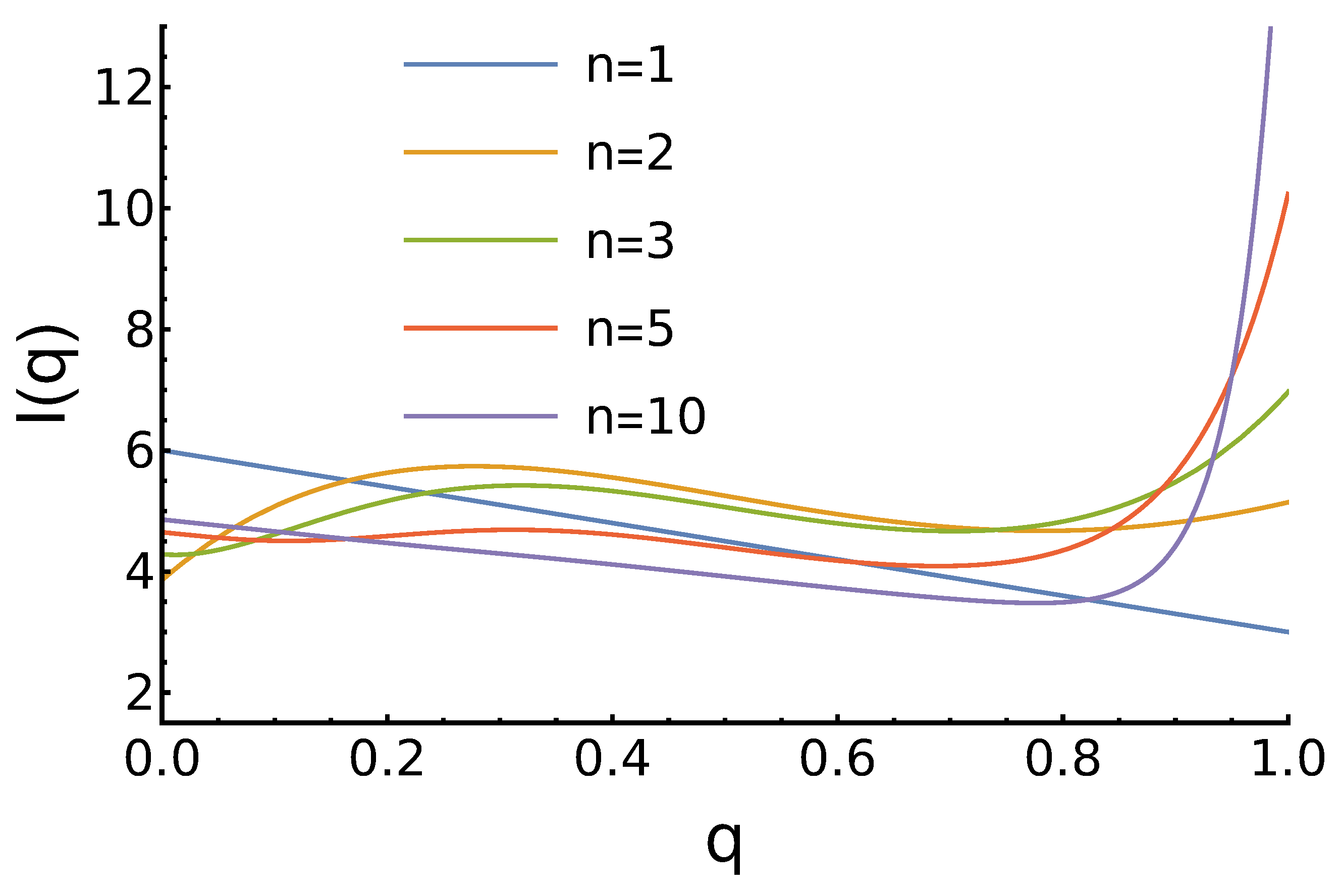
- For , the maximum for is higher as there are more opponents, who prefer to cooperate;
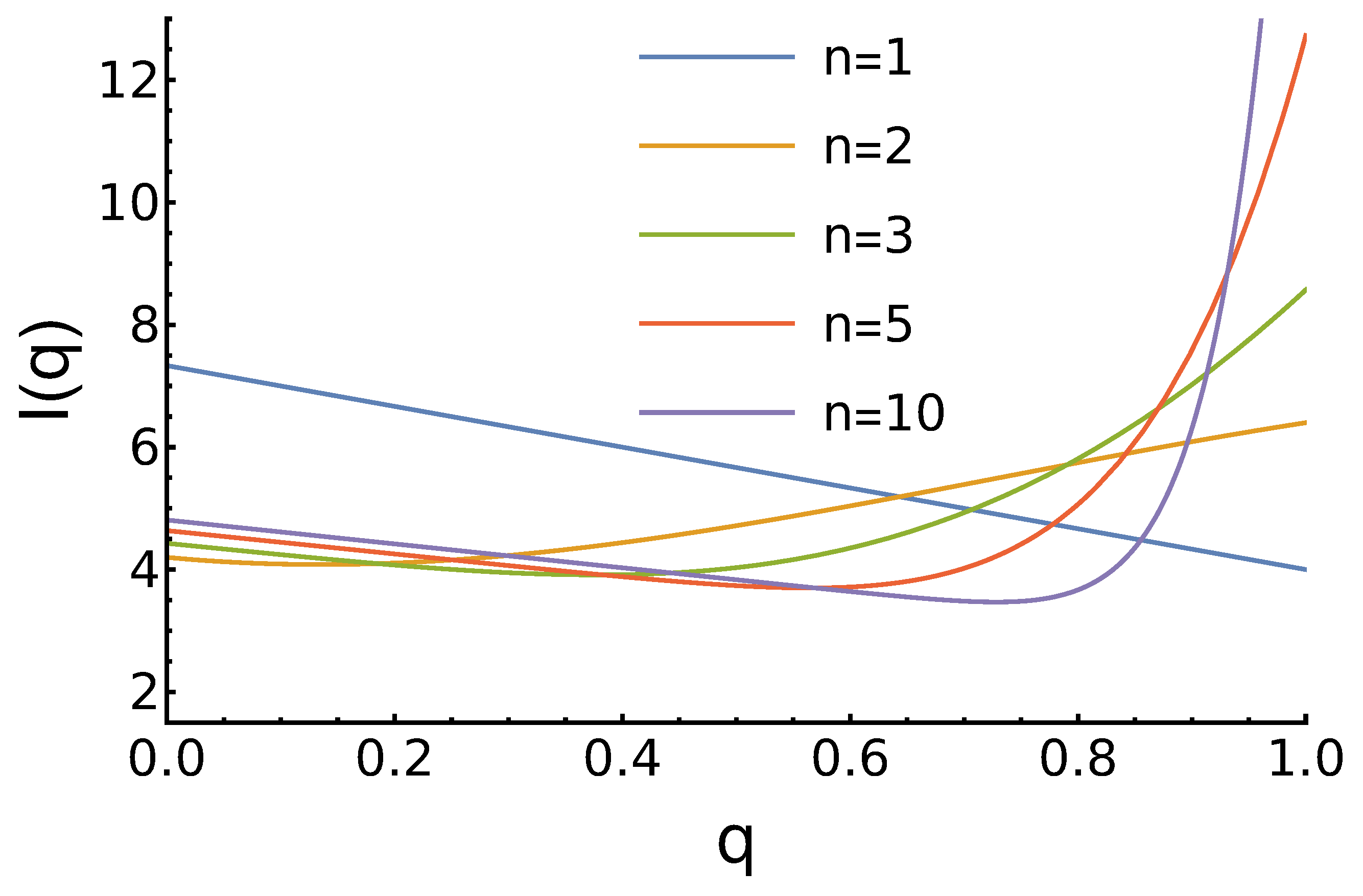
- For , there is no maximum for medium q. In contrast, we observe the minimum near . The position of this minimum shifts to the right as n increases;
- For , the maximum is at and it grows with the increase of n.
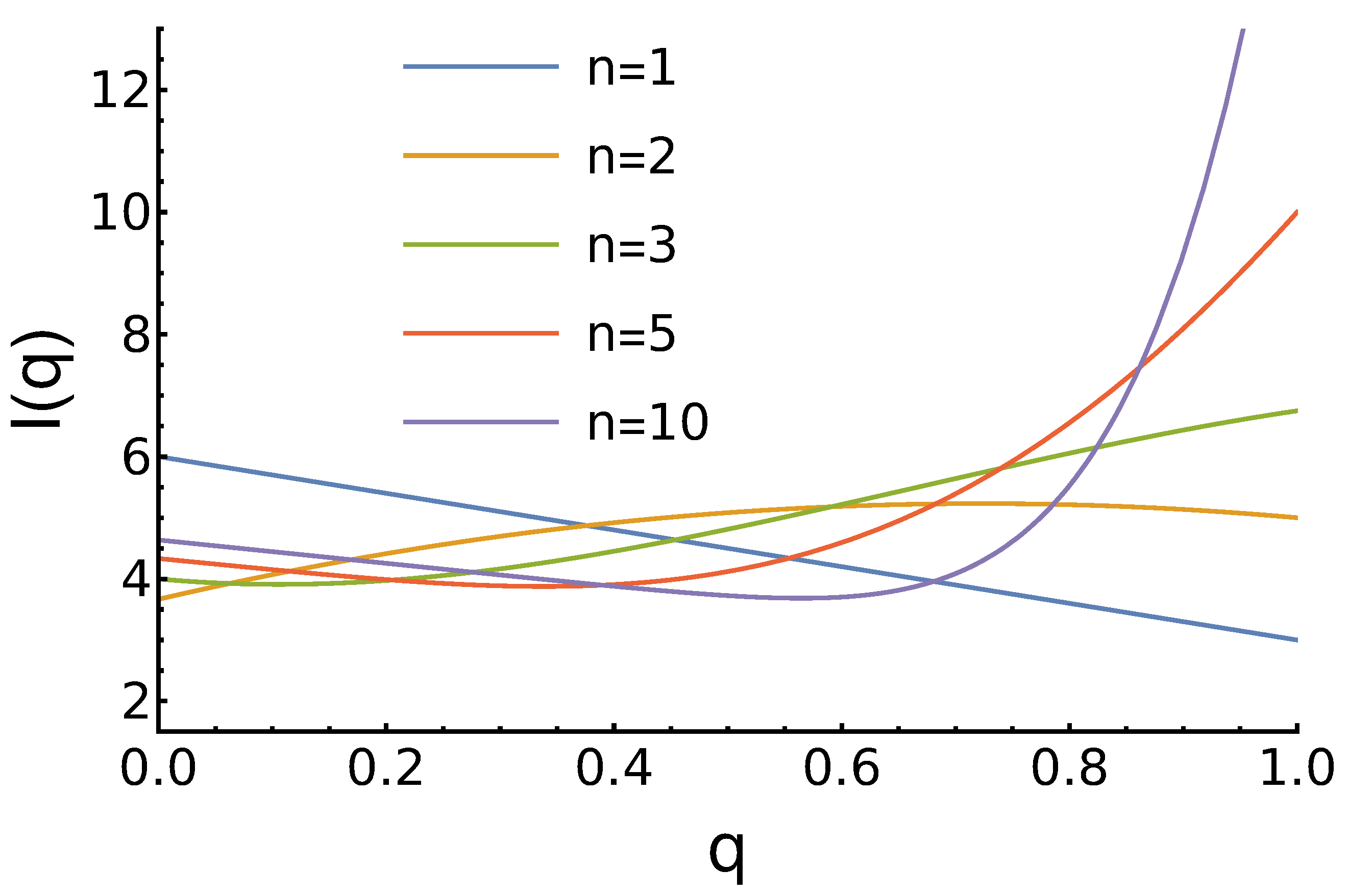
3.3. Case 3: Decreases with an Increase of x
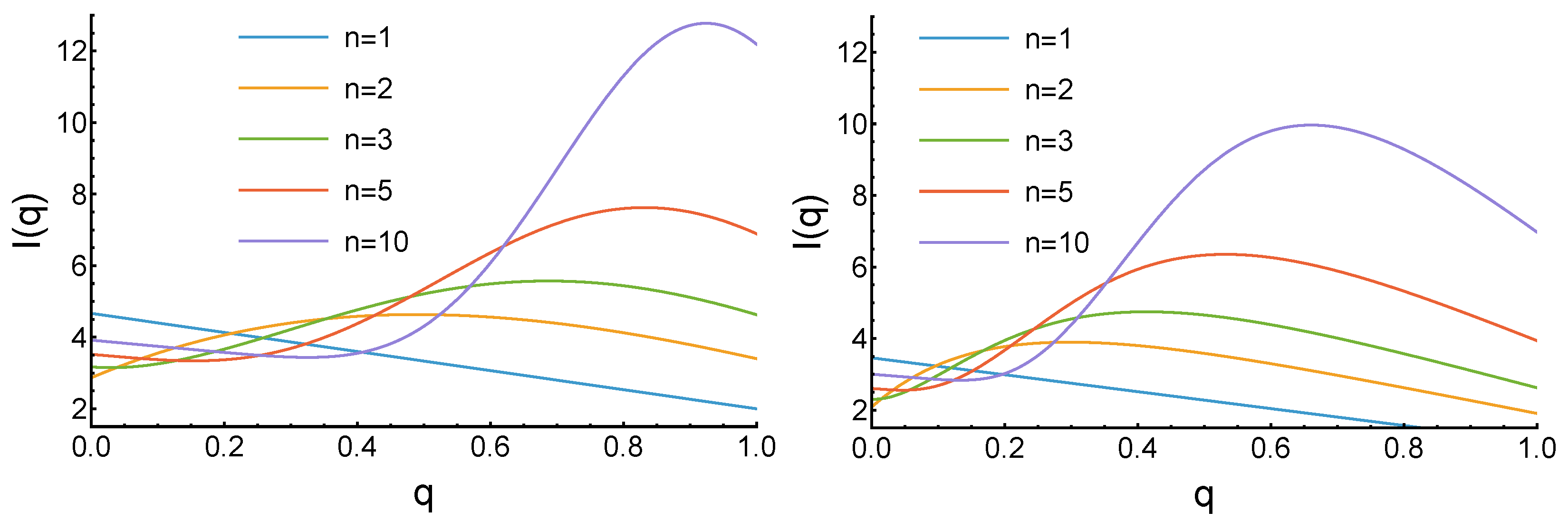
3.4. Case 4: with Maximum at and Minima for
3.5. Case 5: with Minimum at and Maxima for
4. Discussion
5. Conclusions
Supplementary Materials
Funding
Institutional Review Board Statement
Informed Consent Statement
Data Availability Statement
Acknowledgments
Conflicts of Interest
Abbreviations
| PD | Prisoner’s Dilemma |
| IPD | Iterated Prisoner’s Dilemma |
References
- Rapoport, A.; Chammah, A.M. Prisoner’s Dilemma: A Study in Conflict and Cooperation; University of Michigan Press: Ann Arbor, MI, USA, 1965; Volume 165. [Google Scholar]
- Axelrod, R. The Evolution of Cooperation; Basic Books: New York, NY, USA, 1984. [Google Scholar]
- Nash, J.F., Jr. Equilibrium points in n-person games. Proc. Natl. Acad. Sci. USA 1950, 36, 48–49. [Google Scholar] [CrossRef] [PubMed]
- Perc, M.; Jordan, J.J.; Rand, D.G.; Wang, Z.; Boccaletti, S.; Szolnoki, A. Statistical physics of human cooperation. Phys. Rep. 2017, 687, 1–51. [Google Scholar] [CrossRef]
- Cooper, R.; DeJong, D.V.; Forsythe, R.; Ross, T.W. Cooperation without Reputation: Experimental Evidence from Prisoner’s Dilemma Games. Games Econ. Behav. 1996, 12, 187–218. [Google Scholar] [CrossRef]
- Press, W.H.; Dyson, F.J. Iterated Prisoner’s Dilemma contains strategies that dominate any evolutionary opponent. Proc. Natl. Acad. Sci. USA 2012, 109, 10409–10413. [Google Scholar] [CrossRef] [PubMed]
- Hilbe, C.; Nowak, M.A.; Sigmund, K. Evolution of extortion in iterated prisoner’s dilemma games. Proc. Natl. Acad. Sci. USA 2013, 110, 6913–6918. [Google Scholar] [CrossRef]
- Wang, Z.; Zhou, Y.; Lien, J.W.; Zheng, J.; Xu, B. Extortion can outperform generosity in the iterated prisoner’s dilemma. Nat. Commun. 2016, 7, 11125. [Google Scholar] [CrossRef]
- Dal Bó, P.; Fréchette, G.R. Strategy Choice in the Infinitely Repeated Prisoner’s Dilemma. Am. Econ. Rev. 2019, 109, 3929–3952. [Google Scholar] [CrossRef]
- Mieth, L.; Buchner, A.; Bell, R. Moral labels increase cooperation and costly punishment in a Prisoner’s Dilemma game with punishment option. Sci. Rep. 2021, 11, 10221. [Google Scholar] [CrossRef] [PubMed]
- Gong, Y.; Liu, S.; Bai, Y. Reputation-based co-evolutionary model promotes cooperation in prisoner’s dilemma game. Phys. Lett. A 2020, 384, 126233. [Google Scholar] [CrossRef]
- Gächter, S.; Lee, K.; Sefton, M.; Weber, T.O. The role of payoff parameters for cooperation in the one-shot Prisoner’s Dilemma. Eur. Econ. Rev. 2024, 166, 104753. [Google Scholar] [CrossRef]
- You, T.; Zhang, H.; Zhang, Y.; Li, Q.; Zhang, P.; Yang, M. The influence of experienced guider on cooperative behavior in the Prisoner’s dilemma game. Appl. Math. Comput. 2022, 426, 127093. [Google Scholar] [CrossRef]
- Yang, Z.; Zheng, L.; Perc, M.; Li, Y. Interaction state Q-learning promotes cooperation in the spatial prisoner’s dilemma game. Appl. Math. Comput. 2024, 463, 128364. [Google Scholar] [CrossRef]
- Dong, Y.; Sun, S.; Xia, C.; Perc, M. Second-Order Reputation Promotes Cooperation in the Spatial Prisoner’s Dilemma Game. IEEE Access 2019, 7, 82532–82540. [Google Scholar] [CrossRef]
- Pfeiffer, T.; Tran, L.; Krumme, C.; Rand, D.G. The value of reputation. J. R. Soc. Interface 2012, 9, 2791–2797. [Google Scholar] [CrossRef]
- Gong, B.; Yang, C.L. Reputation and Cooperation: An Experiment on Prisoner’s Dilemma with Second-Order Information. 2010. Available online: https://papers.ssrn.com/sol3/papers.cfm?abstract_id=1549605 (accessed on 13 June 2025).
- Lu, P.; Wang, F. Heterogeneity of inferring reputation probability in cooperative behaviors for the spatial prisoners’ dilemma game. Phys. A Stat. Mech. Its Appl. 2015, 433, 367–378. [Google Scholar] [CrossRef]
- Samu, F.; Számadó, S.; Takács, K. Scarce and directly beneficial reputations support cooperation. Sci. Rep. 2020, 10, 11486. [Google Scholar] [CrossRef]
- Nowak, M.A.; May, R.M. Evolutionary games and spatial chaos. Nature 1992, 359, 826–829. [Google Scholar] [CrossRef]
- Benko, T.P.; Pi, B.; Li, Q.; Feng, M.; Perc, M.; Blažun Vošner, H. Evolutionary games for cooperation in open data management. Appl. Math. Comput. 2025, 496, 129364. [Google Scholar] [CrossRef]
- Cuesta, J.A.; Gracia-Lázaro, C.; Ferrer, A.; Moreno, Y.; Sánchez, A. Reputation drives cooperative behaviour and network formation in human groups. Sci. Rep. 2015, 5, 7843. [Google Scholar] [CrossRef]
- Trivers, R.L. The evolution of reciprocal altruism. Q. Rev. Biol. 1971, 46, 35–57. [Google Scholar] [CrossRef]
- Bao, A.R.H.; Liu, Y.; Dong, J.; Chen, Z.P.; Chen, Z.J.; Wu, C. Evolutionary Game Analysis of Co-Opetition Strategy in Energy Big Data Ecosystem under Government Intervention. Energies 2022, 15, 2066. [Google Scholar] [CrossRef]
- Axelrod, R.; Hamilton, W.D. The Evolution of Cooperation. Science 1981, 211, 1390–1396. [Google Scholar] [CrossRef]
- Nowak, M.A.; May, R.M. Tit for tat in heterogeneous populations. Nature 1992, 355, 250–253. [Google Scholar] [CrossRef]
- Parsons, S.D.; Gymtrasiewicz, P.; Wooldridge, M. Game Theory and Decision Theory in Agent-Based Systems; Springer Science & Business Media: New York, NY, USA, 2012; Volume 5. [Google Scholar]
- Chen, S.H. Agent-Based Computational Economics: How the Idea Originated and Where It Is Going; Routledge: London, UK, 2017. [Google Scholar]
- Cieśla, M.; Snarska, M. A simple mechanism causing wealth concentration. Entropy 2020, 22, 1148. [Google Scholar] [CrossRef] [PubMed]
- Gray, J.; Hicks, R.P. Reputations, perceptions, and international economic agreements. Int. Interact. 2014, 40, 325–349. [Google Scholar] [CrossRef]
- Chen, S.H.; Xiao, H.; Huang, W.d.; He, W. Cooperation of Cross-border E-commerce: A reputation and trust perspective. J. Glob. Inf. Technol. Manag. 2022, 25, 7–25. [Google Scholar] [CrossRef]
- Liberman, V.; Samuels, S.M.; Ross, L. The name of the game: Predictive power of reputations versus situational labels in determining prisoner’s dilemma game moves. Personal. Soc. Psychol. Bull. 2004, 30, 1175–1185. [Google Scholar] [CrossRef] [PubMed]
- Eshel, I.; Cavalli-Sforza, L.L. Assortment of encounters and evolution of cooperativeness. Proc. Natl. Acad. Sci. USA 1982, 79, 1331–1335. [Google Scholar] [CrossRef]
- Izquierdo, S.S.; Izquierdo, L.R.; Hauert, C. Positive and negative selective assortment. J. Theor. Biol. 2025, 608, 112129. [Google Scholar] [CrossRef]
- Bergstrom, T.C. The Algebra of Assortative Encounters and the Evolution of Cooperation. Int. Game Theory Rev. 2003, 05, 211–228. [Google Scholar] [CrossRef]
- Feng, M.; Pi, B.; Deng, L.J.; Kurths, J. An Evolutionary Game With the Game Transitions Based on the Markov Process. IEEE Trans. Syst. Man Cybern. Syst. 2024, 54, 609–621. [Google Scholar] [CrossRef]
- Taylor, C.; Nowak, M.A. Evolutionary game dynamics with non-uniform interaction rates. Theor. Popul. Biol. 2006, 69, 243–252. [Google Scholar] [CrossRef] [PubMed]
- Glynatsi, N.E.; Knight, V.; Harper, M. Properties of winning Iterated Prisoner’s Dilemma strategies. PLoS Comput. Biol. 2024, 20, e1012644. [Google Scholar] [CrossRef]
- Li, Q.; Zhao, G.; Feng, M. Prisoner’s dilemma game with cooperation-defection dominance strategies on correlational multilayer networks. Entropy 2022, 24, 822. [Google Scholar] [CrossRef] [PubMed]
- Perc, M.c.v.; Szolnoki, A. Social diversity and promotion of cooperation in the spatial prisoner’s dilemma game. Phys. Rev. E 2008, 77, 011904. [Google Scholar] [CrossRef]
- Pi, B.; Feng, M.; Deng, L.J. A memory-based spatial evolutionary game with the dynamic interaction between learners and profiteers. Chaos Interdiscip. J. Nonlinear Sci. 2024, 34, 063120. [Google Scholar] [CrossRef]
- Burda, Z.; Krawczyk, M.J.; Malarz, K.; Snarska, M. Wealth rheology. Entropy 2021, 23, 842. [Google Scholar] [CrossRef]
- Kim, Y. The Influence of Conformity and Global Learning on Social Systems of Cooperation: Agent-Based Models of the Spatial Prisoner’s Dilemma Game. Systems 2025, 13, 288. [Google Scholar] [CrossRef]
- Osborne, M.J. An Introduction to Game Theory; Springer: Berlin/Heidelberg, Germany, 2004; Volume 3. [Google Scholar]

| case 1 | 4.50 (0.87) | 4.83 (0.45) | 5.00 (0.94) | 5.17 (1.67) | 5.32 (2.86) |
| case 2 | 5.11 (0.79) | 5.33 (0.71) | 5.42 (1.44) | 5.52 (2.40) | 5.59 (3.94) |
| case 3 (linear) | 3.78 (0.63) | 4.09 (0.51) | 4.27 (0.88) | 4.47 (1.41) | 4.70 (2.25) |
| case 3 (exponential) | 3.03 (0.40) | 3.25 (0.55) | 3.41 (0.87) | 3.60 (1.28) | 3.87 (1.89) |
| case 4 | 4.50 (0.67) | 4.76 (0.63) | 4.89 (1.19) | 5.02 (1.95) | 5.16 (3.16) |
| case 5 | 4.50 (1.16) | 4.95 (0.43) | 5.14 (0.71) | 5.32 (1.48) | 5.43 (2.76) |
Disclaimer/Publisher’s Note: The statements, opinions and data contained in all publications are solely those of the individual author(s) and contributor(s) and not of MDPI and/or the editor(s). MDPI and/or the editor(s) disclaim responsibility for any injury to people or property resulting from any ideas, methods, instructions or products referred to in the content. |
© 2025 by the author. Licensee MDPI, Basel, Switzerland. This article is an open access article distributed under the terms and conditions of the Creative Commons Attribution (CC BY) license (https://creativecommons.org/licenses/by/4.0/).
Share and Cite
Cieśla, M. Reputation in the Iterated Prisoner’s Dilemma: A Simple, Analytically Solvable Agents’ Model. Entropy 2025, 27, 639. https://doi.org/10.3390/e27060639
Cieśla M. Reputation in the Iterated Prisoner’s Dilemma: A Simple, Analytically Solvable Agents’ Model. Entropy. 2025; 27(6):639. https://doi.org/10.3390/e27060639
Chicago/Turabian StyleCieśla, Michał. 2025. "Reputation in the Iterated Prisoner’s Dilemma: A Simple, Analytically Solvable Agents’ Model" Entropy 27, no. 6: 639. https://doi.org/10.3390/e27060639
APA StyleCieśla, M. (2025). Reputation in the Iterated Prisoner’s Dilemma: A Simple, Analytically Solvable Agents’ Model. Entropy, 27(6), 639. https://doi.org/10.3390/e27060639