


Disentanglement—Induced Superconductivity


Andrew and Erna Viterbi Department of Electrical Engineering, Technion, Haifa 32000, Israel
Entropy 2025, 27(6), 630; https://doi.org/10.3390/e27060630
Submission received: 22 April 2025
/
Revised: 5 June 2025
/
Accepted: 12 June 2025
/
Published: 13 June 2025
(This article belongs to the Special Issue Quantum Entanglement—Second Edition)
Abstract
:The current study is motivated by a difficulty in reconciling between particle number conservation and superconductivity. An alternative modeling, which is based on the hypothesis that disentanglement spontaneously ocuurs in quantum systems, is explored. The Fermi–Hubbard mode is employed to demonstrate a disentanglement-induced quantum phase transition into a state with a finite superconducting order parameter. Moreover, the effect of disentanglement on Josephson junction’s current phase relation is explored
Keywords:
disentanglement1. Introduction
In the Bardeen, Cooper, and Schrieffer (BCS) model [1], the Hamiltonian of electrons in a superconducting metal contains interaction terms proportional to the operators , where is a pair annihilation operators, and annihilates a single particle Fermionic state having momentum and spin state . The operator can be expressed as , where is the expectation value of in thermal equilibrium, and . In the mean field approximation (MFA), the term is disregarded [see Equation (18.307) of Ref. [2]]. This approximation leads to a mean field Hamiltonian , which can be analytically diagonalized by implementing a Bogoliubov transformation.
The MFA greatly simplifies the many-body problem under study; however, it yields some predictions that are arguably inconsistent with what is expected from the original Hamiltonian . Particle number is conserved by , and consequently, it is expected that in steady state, . In contrast, , which is proportional to the BCS energy gap, can become finite in the MFA. Moreover, the ground state of the mean-field Hamiltonian is continuously degenerate, whereas the ground state of the BCS Hamiltonian is generically non-degenerate. The question of MFA validity is related to the spontaneous symmetry breaking in the Higgs mechanism [3].
It was pointed out that the MFA can be, at least partially, justified in the thermodynamical limit. Particle number conservation implies that in steady states, where is the pair number operator. In general, the MFA allows the violation of this conservation law (i.e., it allows non-zero values of in steady state). However, it was shown that in the MFA, both and are proportional to the volume of the system [4], and thus, the violation of particle number conservation becomes insignificant in the thermodynamical limit. The mean field approach has been supported in Ref. [5] by showing that the Ginzburg–Levanyuk parameter is typically small for electrons in metals. Moreover, it was argued in Ref. [6] that the BCS interaction between pairs has an infinite range, and consequently exact solution of the BCS Hamiltonian can be derived using a MFA. It was shown in Ref. [7] that the Bogoliubov inequality, together with a variational calculation and some assumptions, can lead to the MFA Hamiltonian . Another attempt to rigorously derive the MFA Hamiltonian , which is based on Wick’s theorem [8], has been presented in [9,10]. However, this derivation employs a relation, which can be derived from Wick’s theorem only for the case of Gaussian states [see Equation (16.131) of Ref. [2]]. In contrast, the thermal equilibrium state that is derived from the BCS Hamiltonian is generically non-Gaussian.
The current study is motivated by the arguably limited range of validity of the MFA, and by the difficulty in reconciling between the spontaneous symmetry breaking occurring in the superconducting state, and particle number conservation [11,12,13]. An alternative approach, which is based on a recently proposed hypothesis that disentanglement spontaneously occurs in quantum systems, is explored. As is shown below, the conjecture that disentanglement plays a role in superconductivity is falsifiable, since it yields predictions that are distinguishable from what is derived from MFA-based models. In the current study, the Fermi–Hubbard model [14,15,16,17,18,19,20,21,22,23] is employed to study the effect of disentanglement on both superconducting order parameter and current-phase relation (CPR) of a weak link [24].
2. Disentanglement
According to the spontaneous disentanglement hypothesis, time evolution for the reduced density operator is governed by a modified master equation given by [25,26,27,28,29]
where ℏ is the Planck’s constant, is the Hamiltonian, the operator is allowed to depend on , and . The operator is given by , where both rates and are positive, and both operators and are Hermitian. The operator , which gives rise to thermalization [30,31], is given by , where is the Helmholtz free energy operator [32], is the thermal energy inverse, is the Boltzmann’s constant, and T is the temperature.
For the case of a system composed of indistinguishable particles, the disentanglement operator is derived from two–particle interaction (TPI) [33]. The term in the Hamiltonian accounting for TPI is denoted by . In a basis that diagonalizes the TPI, the operator is expressed in terms of the operators , where is a number operator associated with the j’th single-particle state. In that basis, each term in proportional to contributes to , a term proportional to , where . The term gives rise to suppression of , with a rate proportional to , where the covariance is defined by [see Equation (1)]. Alternatively, the covariance can be expressed as , where is the probability that state j is occupied, and is the probability that states and are both occupied.
3. Fermi–Hubbard Model
Consider an array of sites occupied by Fermions. Single-site occupation energy, nearest neighbors hopping, and TPI are characterized by the real parameters , t, and U, respectively. The creation and annihilation operators corresponding to site l with spin state are denoted by and , respectively. The operators and satisfy Fermionic anti-commutation relations. The Fermi–Hubbard Hamiltonian is given by , where the single-particle part is
where denotes that and are nearest neighbors, the TPI part is given by
and the Fermionic number operator is given by .
The term in the TPI part [see Equation (3)] can be expressed as , where . In the MFA, i.e., when the term is disregarded, it is well known that the Fermi–Hubbard model supports a superconducting phase for particular realizations [34].
As was discussed above, disentanglement gives rise to the suppression of the covariance . In the rapid disentanglement approximation [35], it is assumed that the rate of disentanglement is sufficiently large to allow disregarding the term . In this limit, the disentanglement-based model yields predictions that are identical to what is derived from the standard (i.e., without disentanglement) Fermi–Hubbard model, when the MFA is implemented, and thus, the disentanglement-based model in this limit can account for superconductivity, in the same way that the mean field Fermi–Hubbard model can.
In the current study, the effect of disentanglement is explored, without assuming that is sufficiently large to validate the rapid disentanglement approximation. As is demonstrated below, for some cases, analytical results can be derived from the modified master Equation (1), provided that the size of the under study system is kept sufficiently small. However, since the rapid disentanglement approximation is not implemented, analysis commonly becomes intractable in the macroscopic limit.
For the relatively simple systems to be discussed below, it is assumed that the Fermi–Hubbard array is one-dimensional; the number of sites, which is denoted by L, is finite; and the array has a ring configuration; thus, the last () hopping term [see Equation (2)] is taken to be given by .
4. Truncation Approximation
For some cases, dynamics governed by the modified master Equation (1) can be simplified by implementing a truncation approximation. In this approximation, the operators and are replaced by and , respectively, where P is a projection operator. For a two-level truncation approximation, the projection is expressed as , where and are two orthonormal state vectors (i.e., and ). The density operator for that case is expressed in terms of the real vector as
where is the Pauli matrix vector. Similarly, the Hamiltonian is expressed as , where is real. It is assumed that , where , and both the number and the vector are real.
The entropy operator can be expressed as , where and , and the operator as , where , , and [recall the identity , and note that the Pauli matrices are all trace-less]. The modified master Equation (1) yields an equation of motion for , given by
Note that, generally, depends on , and that the vector is orthogonal to , provided that (i.e., represents a pure state, for which ).
When the Hamiltonian is time-independent, steady-state solutions of the modified master Equation (1) occur at extremum points of an effective free energy , which is given by . In the truncation approximation, , where
and . For a constant , the Helmholtz free energy is minimized at the thermal equilibrium point , where the unit vector is given by [note that ].
For the under-study Fermi–Hubbard model, and for the case of a two-site array (i.e., ) and , a two-level truncation approximation, which is based on a projection onto the subspace spanned by the floor (i.e., ground) and ceiling energy eigenstates, becomes applicable, provided that [33]. For the case , the floor and ceiling states are given by and , where , , , and denotes a normalized state, where , , and . Note that the disentanglement expectation value with respect to the state , where the angle is real, is given by . Hence, in the limit , for which and , the combined state is nearly fully disentangled.
The relations , and , where , enables an analytical evaluation of the effective free energy . The result reveals that in the low-temperature limit, and for , a symmetry-breaking quantum phase transition occurs for this case at . The dependency on the ratio of steady-state values of (a) the normalized energy expectation value and (b) purity is shown in Figure 1. The steady-state values are calculated by numerically integrating the modified master Equation (1) (without employing the truncation approximation). The plot in Figure 1b reveals that the purity drops below unity above the phase transition occurring at .
5. Order Parameter
The plot in Figure 2 demonstrates the time evolution of the vector for the case [the truncation approximation is not being employed for the numerical integration of the modified master Equation (1)]. The vector operator is given by , where , and where . The following holds , , and , where and where , and thus (note that ). The variable represents an order parameter.
In the low-temperature limit, and in the absence of disentanglement (i.e., for ), the ground state density operator is a steady-state solution of the modified master Equation (1). Note that for the ground state . Above the disentanglement-induced quantum phase transition, i.e., for , the ground state becomes unstable. For the assumed parameters’ values used to generate the plot in Figure 2, the ratio is 50 (see figure caption). The plot shows time evolution for 16 different initial pure states, denoted by , where is given by , where [i.e., ]. Time evolution, which is obtained by numerically integrating the modified master Equation (1), is shown for 16 equally spaced values for the angle in the range . The plot demonstrates that the steady-state value of (labelled in Figure 2 by red × symbols) that is obtained with the initial state is parallel to the unit vector . Thus, for this one-dimensional model, a disentanglement-induced spontaneous symmetry breaking, which occurs for , gives rise to finite values of the order parameter .
6. CPR
For the case where the one-dimensional array is occupied by spinless Fermions, the Hamiltonian is expressed as
The Fermionic creation and annihilation operators corresponding to site are denoted by and , respectively, and the operator is given by and . It is assumed that and (i.e., all nearest neighbor site pairs, except for the pair , share the same coefficients, and ). The single-site occupation energy , hopping amplitudes t and , the phases , and the pairing amplitudes g and are all real constants. For the case of an opened chain, and , whereas and for the case of a closed ring.
The term can be expressed as , where . In the MFA, for which the term is disregarded, the resultant Hamiltonian, which is denoted by , describes a Kitaev one-dimensional array [36]. Note that the total number of particles is conserved by [see Equation (7)], whereas only the total number mod 2 is conserved by . In the analysis below, the MFA, which generally enables violation of number conservation, is not implemented.
Consider the case where a magnetic flux given by is externally applied to the ring’s hole, where is real and is the flux quantum (Planck’s constant, vacuum speed of light, and electronic charge are denoted by h, c, and e, respectively). The effect of the applied flux is taken into account by setting the phases in the Hamiltonian (7) according to for and [37,38]. The circulating current is calculated using the relation [see Equation (18.142) of Ref. [2]], where the steady-state energy expectation value is evaluated by numerically integrating the modified master Equation (1). For the current case, the disentanglement operator is given by , where (note that and , where ).
The effect of disentanglement on CPR is demonstrated by the plots shown in Figure 3. The assumed rate of disentanglement for the plots in (a) and (b) is , and , respectively. For comparison, the plot in Figure 3c displays the Beenakker–VanHouten CPR [39,40], which was calculated for a single short channel of transmission , and which is given by , where denotes the critical current, and [see Equation (A4) of Ref. [41]]
The most pronounced effect of disentanglement on the CPR are the sharp features seen in Figure 3a,b near half-integer values of the normalized applied flux . These features do not violate the symmetry relation , where n is an integer. Note that some unexplained features obeying the same symmetry are visible in some spectral measurements of Josephson devices (e.g., see Figures 2 and 4 of [42], Figure 2 of [43], and Figure 2 of [44]). Further study is needed to determine whether disentanglement can account for such experimentally observed features. Note that a variety of unconventional mechanisms, including topological and multi-band superconductivity, can give rise to CPR having features that resemble what is seen in Figure 3a,b (e.g., see Ref. [45]).
7. Effective Free Energy
Disentanglement is explored below by evaluating the effective free energy for the spinless one-dimensional array in an open chain configuration. The energy eigenvalues of [see Equation (7)] are shown as a function of in Figure 4a, for the case where , , and . For , where [see the black dashed vertical line in Figure 4a], the ground state is the one-particle state [see the blue line in Figure 4a], whereas the two-particle state [see the red line in Figure 4a] becomes the ground state for .
Consider a reduced-density operator having matrix representation in the basis given by , where is real. The truncated density operator can be used for approximately calculating the effective free energy for . The dependency of on and for the value [see the green dashed vertical line in Figure 4a] is shown in Figure 4b (note that does not depend on and on in the truncation approximation). The color-coded plot of reveals a disentanglement-induced transition from monostability to bistability. In the low-temperature limit, and in the absence of disentanglement [i.e., in the limit ], the effective free energy is minimized for the two-particle state . However, for , the system becomes bistable [see Figure 4b].
8. Summary
Spontaneous disentanglement allows the violation of particle number conservation, which, in turn, enables a quantum phase transition induced by symmetry breaking. The Hubbard–Fermi model is employed for studying the effect of disentanglement on the superconducting order parameter and on the CPR of a weak link. While the current study is focused on exploring the effect of disentanglement on small systems, future research will explore the macroscopic limit using stability analysis [46] (this research direction has been proposed by one of the reviewers of this paper). Moreover, more realistic theoretical models that can yield experimentally testable predictions will be developed.
Funding
This research received no external funding.
Institutional Review Board Statement
Not applicable.
Data Availability Statement
Data are contained within the article.
Conflicts of Interest
The author declares no conflicts of interest.
References
- Bardeen, J.; Cooper, L.N.; Schrieffer, J.R. Theory of superconductivity. Phys. Rev. 1957, 108, 1175. [Google Scholar] [CrossRef]
- Buks, E. Quantum Mechanics—Lecture Notes. 2025. Available online: http://buks.net.technion.ac.il/teaching/ (accessed on 11 June 2025).
- Mannheim, P.D. Colloquium on the higgs boson. arXiv 2015, arXiv:1506.04120. [Google Scholar]
- De Gennes, P.-G. Superconductivity of Metals and Alloys; CRC Press: Boca Raton, FL, USA, 2018. [Google Scholar]
- Zyuzin, A.A.; Zyuzin, A.Y. Superconductivity from incoherent cooper pairs in strong-coupling regime. arXiv 2023, arXiv:2308.04508. [Google Scholar] [CrossRef]
- Coleman, P. Introduction to Many-Body Physics; Cambridge University Press: Cambridge, UK, 2015. [Google Scholar]
- Kuzemsky, A.L. Variational principle of bogoliubov and generalized mean fields in many-particle interacting systems. Int. J. Mod. Phys. B 2015, 29, 1530010. [Google Scholar] [CrossRef]
- Gaudin, M. Une démonstration simplifiée du théoreme de wick en mécanique statistique. Nucl. Phys. 1960, 15, 89–91. [Google Scholar] [CrossRef]
- Kainth, M. Superconductivity and Mean Field Distribution Theory on a Hubbard Model with Local Symmetries. Ph.D. Thesis, University of Birmingham, Birmingham, UK, 2020. [Google Scholar]
- Kainth, M.; Long, M.W. A rigorous demonstration of superconductivity in a repulsive hubbard model. arXiv 2019, arXiv:1904.07138. [Google Scholar]
- Lin, Y.; Leggett, A.J. Some questions concerning majorana fermions in 2d (p+ ip) fermi superfluids. Quantum Front. 2022, 1, 4. [Google Scholar] [CrossRef]
- Lapa, M.F.; Levin, M. Rigorous results on topological superconductivity with particle number conservation. Phys. Rev. Lett. 2020, 124, 257002. [Google Scholar] [CrossRef]
- Ortiz, G.; Dukelsky, J.; Cobanera, E.; Esebbag, C.; Beenakker, C. Many-body characterization of particle-conserving topological superfluids. Phys. Rev. Lett. 2014, 113, 267002. [Google Scholar] [CrossRef]
- Bogolyubov, N.M.; Korepin, V.E. The mechanism of cooper pairing in the one-dimensional hubbard model. Stat. Mech. Theory Dyn. Syst. Pap. 1992, 191, 47. [Google Scholar]
- Fabian, J. Ground-state energy of the hubbard model in the bcs approximation. Czechoslov. J. Phys. 1993, 43, 1137–1142. [Google Scholar] [CrossRef]
- Plakida, N.M.; Oudovenko, V.S.; Horsch, P.; Liechtenstein, A.I. Superconducting pairing of spin polarons in the tj model. Phys. Rev. B 1997, 55, R11997. [Google Scholar] [CrossRef]
- Robaszkiewicz, S.; Bułka, B.R. Superconductivity in the hubbard model with pair hopping. Phys. Rev. B 1999, 59, 6430. [Google Scholar] [CrossRef]
- Salwen, N.; Sheets, S.A.; Cotanch, S.R. Bcs and attractive hubbard model comparative study. Phys. Rev. B Condens. Matter Mater. Phys. 2004, 70, 064511. [Google Scholar] [CrossRef]
- Claveau, Y.; Arnaud, B.; Di Matteo, S. Mean-field solution of the hubbard model: The magnetic phase diagram. Eur. J. Phys. 2014, 35, 035023. [Google Scholar] [CrossRef]
- Iemini, F.; Maciel, T.O.; Vianna, R.O. Entanglement of indistinguishable particles as a probe for quantum phase transitions in the extended hubbard model. Phys. Rev. B 2015, 92, 075423. [Google Scholar] [CrossRef]
- Chen, Z.; Li, X.; Ng, T.K. Exactly solvable bcs-hubbard model in arbitrary dimensions. Phys. Rev. Lett. 2018, 120, 046401. [Google Scholar] [CrossRef]
- Xu, D.H.; Yu, Y.C.; Han, X.J.; Chen, X.; Wang, K.; Qin, M.P.; Xiang, T. Phase diagram of the BCS—hubbard model in a magnetic field. Chin. Phys. Lett. 2022, 39, 067403. [Google Scholar] [CrossRef]
- Ferreira, D.L.B.; Maciel, T.O.; Vianna, R.O.; Iemini, F. Quantum correlations, entanglement spectrum, and coherence of the two-particle reduced density matrix in the extended hubbard model. Phys. Rev. B 2022, 105, 115145. [Google Scholar] [CrossRef]
- Golubov, A.A.; Kupriyanov, M.Y.; Il’Ichev, E. The current-phase relation in josephson junctions. Rev. Mod. Phys. 2004, 76, 411–469. [Google Scholar] [CrossRef]
- Kaplan, D.E.; Rajendran, S. Causal framework for nonlinear quantum mechanics. Phys. Rev. D 2022, 105, 055002. [Google Scholar] [CrossRef]
- Geller, M.R. Fast quantum state discrimination with nonlinear positive trace-preserving channels. Adv. Quantum Technol. 2023, 6, 2200156. [Google Scholar] [CrossRef]
- Grimaudo, R.; De Castro, A.; Kuś, M.; Messina, A. Exactly solvable time-dependent pseudo-hermitian su (1, 1) hamiltonian models. Phys. Rev. A 2018, 98, 033835. [Google Scholar] [CrossRef]
- Kowalski, K.; Rembieliński, J. Integrable nonlinear evolution of the qubit. Ann. Phys. 2019, 411, 167955. [Google Scholar] [CrossRef]
- Buks, E. Spontaneous disentanglement and thermalization. Adv. Quantum Technol. 2024, 7, 2400036. [Google Scholar] [CrossRef]
- Grabert, H. Nonlinear relaxation and fluctuations of damped quantum systems. Z. Für Phys. B Condens. Matter 1982, 49, 161–172. [Google Scholar] [CrossRef]
- Öttinger, H.C. Nonlinear thermodynamic quantum master equation: Properties and examples. Phys. Rev. A 2010, 82, 052119. [Google Scholar] [CrossRef]
- Jaynes, E.T. The minimum entropy production principle. Annu. Rev. Phys. Chem. 1980, 31, 579–601. [Google Scholar] [CrossRef]
- Buks, E. Spontaneous disentanglement of indistinguishable particles. Adv. Quantum Technol. 2024, 7, 2400248. [Google Scholar] [CrossRef]
- Arovas, D.P.; Berg, E.; Kivelson, S.A.; Raghu, S. The hubbard model. Annu. Rev. Condens. Matter Phys. 2022, 13, 239–274. [Google Scholar] [CrossRef]
- Buks, E. Disentanglement—Induced bistability in a magnetic resonator. Adv. Quantum Technol. 2025, 2400587. [Google Scholar] [CrossRef]
- Kitaev, A.Y. Unpaired majorana fermions in quantumwires. Physics-Uspekhi 2001, 44, 131. [Google Scholar] [CrossRef]
- Byers, N.; Yang, C.N. Theoretical considerations concerning quantized magnetic flux in superconducting cylinders. Phys. Rev. Lett. 1961, 7, 46. [Google Scholar] [CrossRef]
- Büttiker, M.; Imry, Y.; Landauer, R. Josephson behavior in small normal one-dimensional rings. Phys. Lett. A 1983, 96, 365–367. [Google Scholar] [CrossRef]
- Beenakker, C.W.J.; VanHouten, H. Josephson current through a superconducting quantum point contact shorter than the coherence length. Phys. Rev. Lett. 1991, 66, 3056–3059. [Google Scholar] [CrossRef]
- Beenakker, C.W.J. Universal limit of critical-current fluctuations in mesoscopic josephson junctions. Phys. Rev. Lett. 1991, 67, 3836. [Google Scholar] [CrossRef]
- Segev, E.; Suchoi, O.; Shtempluck, O.; Xue, F.; Buks, E. Metastability in a nano-bridge based hysteretic DC-SQUID embedded in superconducting microwave resonator. Phys. Rev. B 2011, 83, 104507. [Google Scholar] [CrossRef]
- Kurter, C.; Finck, A.D.; Hor, Y.S.; Van Harlingen, D.J. Evidence for an anomalous current—Phase relation in topological insulator josephson junctions. Nat. Commun. 2015, 6, 7130. [Google Scholar] [CrossRef]
- Inomata, K.; Yamamoto, T.; Billangeon, P.M.; Nakamura, Y.; Tsai, J.S. Large dispersive shift of cavity resonance induced by a superconducting flux qubit in the straddling regime. Phys. Rev. B 2012, 86, 140508. [Google Scholar] [CrossRef]
- Buks, E.; Deng, C.; Orgazzi, J.L.F.; Otto, M.; Lupascu, A. Superharmonic resonances in a strongly coupled cavity-atom system. Phys. Rev. A 2016, 94, 033807. [Google Scholar] [CrossRef]
- Kudriashov, A.; Zhou, X.; Hovhannisyan, R.A.; Frolov, A.; Elesin, L.; Wang, Y.; Zharkova, E.V.; Taniguchi, T.; Watanabe, K.; Yashina, L.A.; et al. Non-reciprocal current-phase relation and superconducting diode effect in topological-insulator-based josephson junctions. arXiv 2025, arXiv:2502.08527. [Google Scholar]
- Halperin, B.I. On the hohenberg–mermin–wagner theorem and its limitations. J. Stat. Phys. 2019, 175, 521–529. [Google Scholar] [CrossRef]
Figure 1.
Fermi–Hubbard model. Steady-state values of (a) normalized energy expectation value and (b) purity as a function of the ratio . A symmetry-breaking quantum phase transition occurs at . Assumed parameters’ values are and .
Figure 1.
Fermi–Hubbard model. Steady-state values of (a) normalized energy expectation value and (b) purity as a function of the ratio . A symmetry-breaking quantum phase transition occurs at . Assumed parameters’ values are and .
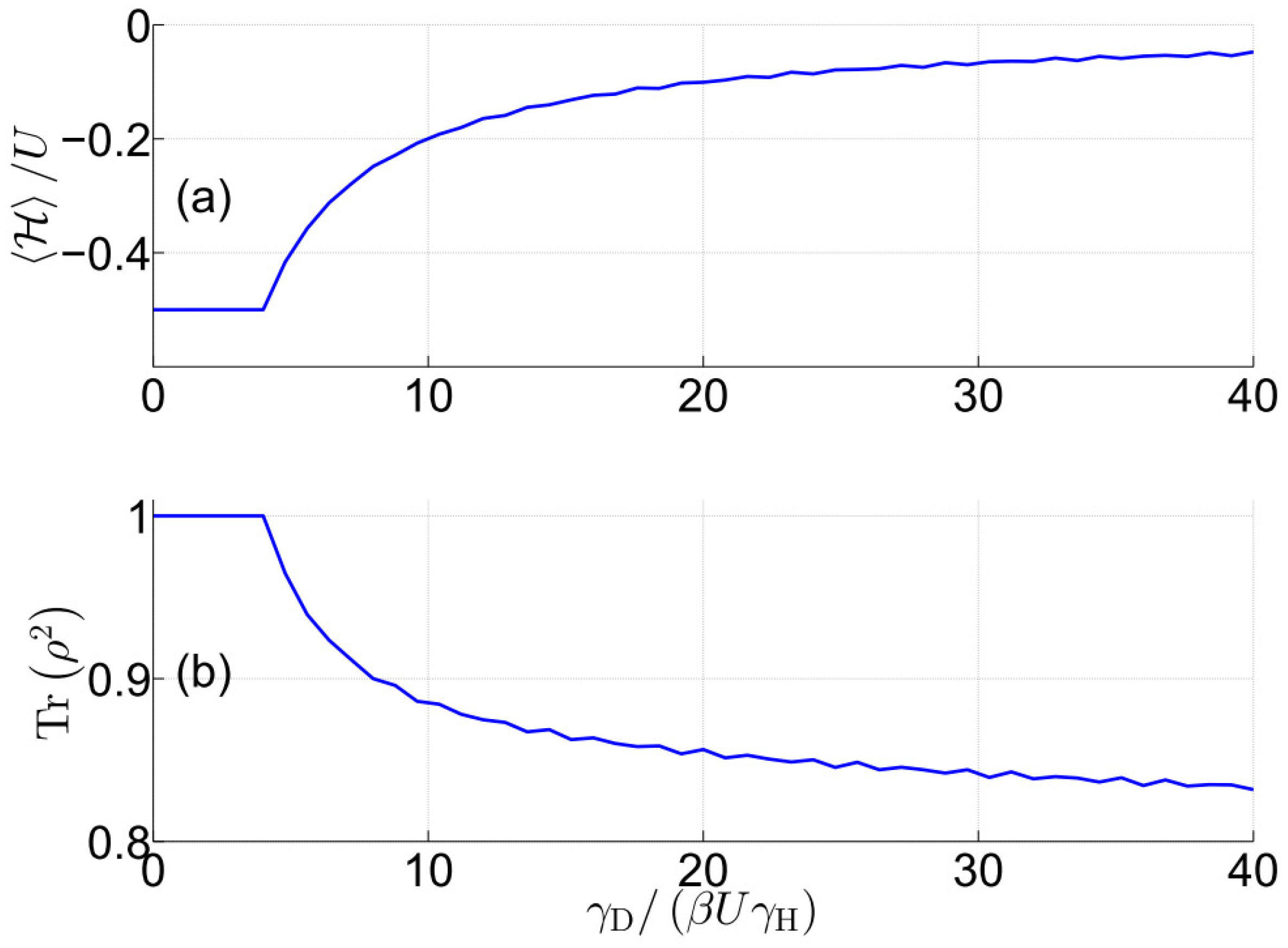
Figure 2.
Disentanglement-induced spontaneous symmetry breaking for the case . Time evolution of the vector for different initial states located close to the ground state [for which ]. The assumed parameters’ values are , , , and .
Figure 2.
Disentanglement-induced spontaneous symmetry breaking for the case . Time evolution of the vector for different initial states located close to the ground state [for which ]. The assumed parameters’ values are , , , and .
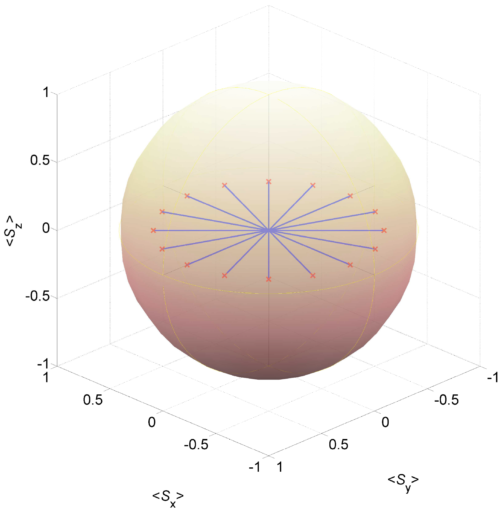
Figure 3.
CPR: The normalized circulating current is shown as a function of normalized applied flux , where is the critical current. The assumed parameters’ values are, , , , , and , for (a,b); , for (a); , for (b); and for (c).
Figure 3.
CPR: The normalized circulating current is shown as a function of normalized applied flux , where is the critical current. The assumed parameters’ values are, , , , , and , for (a,b); , for (a); , for (b); and for (c).
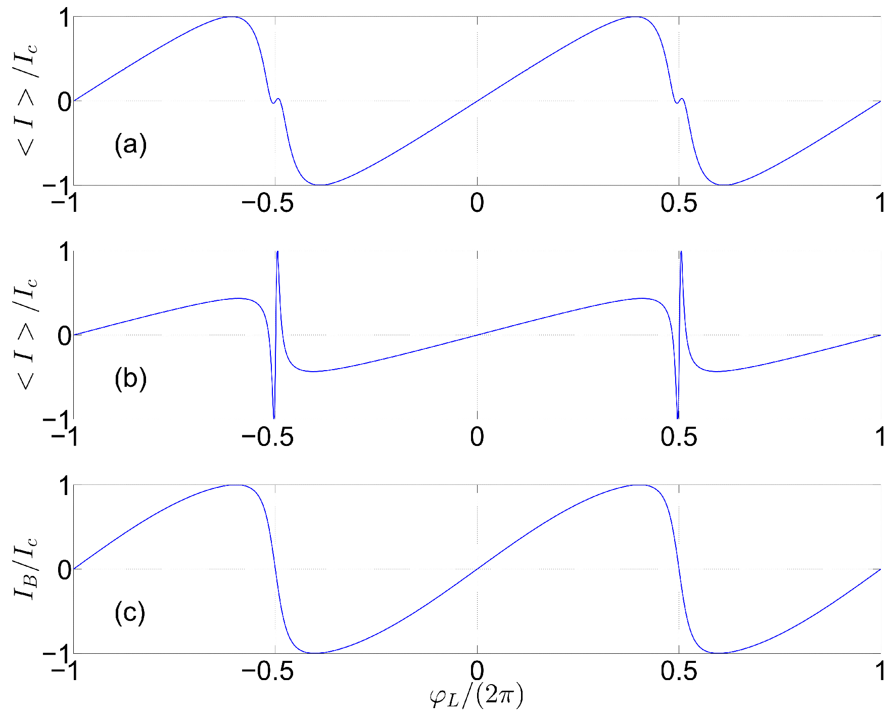
Figure 4.
Effective free energy. Chain parameters are , , and . (a) The energy eigenvalues of (7). (b) The steady-state expectation value .
Figure 4.
Effective free energy. Chain parameters are , , and . (a) The energy eigenvalues of (7). (b) The steady-state expectation value .

Disclaimer/Publisher’s Note: The statements, opinions and data contained in all publications are solely those of the individual author(s) and contributor(s) and not of MDPI and/or the editor(s). MDPI and/or the editor(s) disclaim responsibility for any injury to people or property resulting from any ideas, methods, instructions or products referred to in the content. |
© 2025 by the author. Licensee MDPI, Basel, Switzerland. This article is an open access article distributed under the terms and conditions of the Creative Commons Attribution (CC BY) license (https://creativecommons.org/licenses/by/4.0/).
Share and Cite
MDPI and ACS Style
Buks, E. Disentanglement—Induced Superconductivity. Entropy 2025, 27, 630. https://doi.org/10.3390/e27060630
AMA Style
Buks E. Disentanglement—Induced Superconductivity. Entropy. 2025; 27(6):630. https://doi.org/10.3390/e27060630
Chicago/Turabian StyleBuks, Eyal. 2025. "Disentanglement—Induced Superconductivity" Entropy 27, no. 6: 630. https://doi.org/10.3390/e27060630
APA StyleBuks, E. (2025). Disentanglement—Induced Superconductivity. Entropy, 27(6), 630. https://doi.org/10.3390/e27060630
Note that from the first issue of 2016, this journal uses article numbers instead of page numbers. See further details here.