

Intrinsic and Measured Information in Separable Quantum Processes


Abstract
1. Introduction
1.1. Quantum and Classical Randomness
1.2. Sources with Memory
2. Stochastic Processes
2.1. Classical Processes
2.2. Presentations
- A finite alphabet of m symbols .
- A transition matrix T. That is, if the source emits symbol , with probability , it emits symbol next.
- A finite set of internal states.
- A finite alphabet of m symbols .
- A set of m symbol-labeled transition matrices. That is, if the source is in state , with probability , it emits symbol x while transitioning to state .
2.3. Quantum Processes
2.3.1. Memoryless
2.3.2. Memoryful
2.4. Presentations of Quantum Processes
- A finite set of internal states.
- A finite alphabet of pure qudit states, with each .
- A set of m transition matrices. That is, if the source is in state , with probability , it emits qudit while transitioning to internal state .
2.5. Measured Processes
2.6. Adaptive Measurement Protocols
- A finite set of internal states.
- A unique start state .
- A set of POVMs , one for each internal state.
- An alphabet of m symbols corresponding to different measurement outcomes.
- A deterministic transition map .
2.7. Discussion
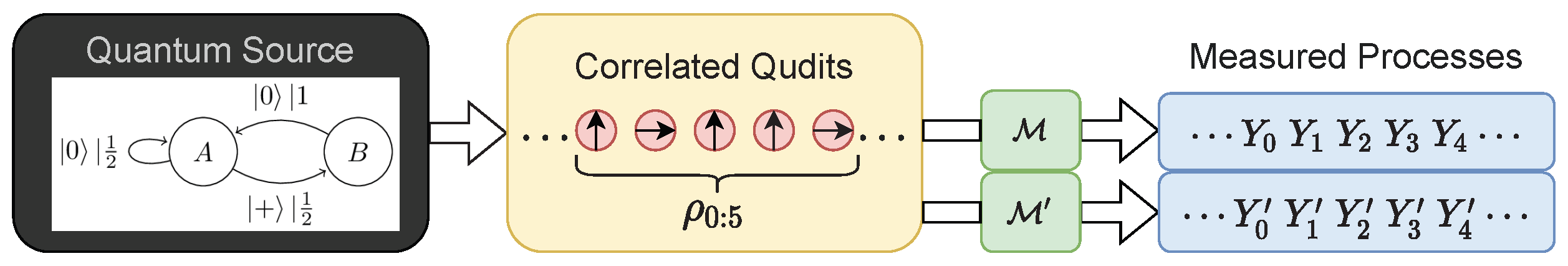
- Given the density matrices describing sequences of ℓ separable qudits, what are the general properties of sequences of measurement outcomes? This is Section 3’s focus. There, ’s quantum information properties bound the classical information properties of measurement sequences for certain classes of measurements.
- Given a hidden Markov chain quantum source, when is an observer with knowledge of the source able to determine the internal state (synchronize)? Can the observer remain synchronized at later times? Section 5 addresses this.
- If an observer encounters an unknown qudit source, how accurately can the observer estimate the informational properties of the emitted process through tomography with limited resources? How can they build approximate models of the source if they reconstruct for some finite ℓ? This is Section 6’s subject.
3. Information in Quantum Processes
3.1. von Neumann Entropy
3.2. Quantum Block Entropy
3.3. von Neumann Entropy Rate
3.4. Quantum Redundancy
3.5. Quantum Entropy Gain
3.6. Quantum Predictability Gain
3.7. Total Quantum Predictability
3.8. Quantum Excess Entropy
3.9. Quantum Transient Information
3.10. Quantum Markov Order
- trivially if consists of orthogonal states, in which case they have identical block entropy curves via Proposition 3.
- if and all symbols in are mapped to the same pure state . In this case, , as the resulting process is i.i.d.
- when , , and consists of nonorthogonal states. Frequently, , since arbitrary sequences of nonorthogonal states cannot reliably be distinguished with a finite POVM.
- if is a separable process with an orthogonal alphabet and uses a POVM whose operators include a projector for each element in via Proposition 4.
- if consists of orthogonal states, , and is a repeated rank-one POVM that does not include projectors onto the states in .
- if and is a repeated POVM measurement with the one-element POVM, . Note that this is not a rank-one POVM.
4. Qudit Processes
4.1. I.I.D. Processes
4.2. Quantum Presentations of Classical Processes
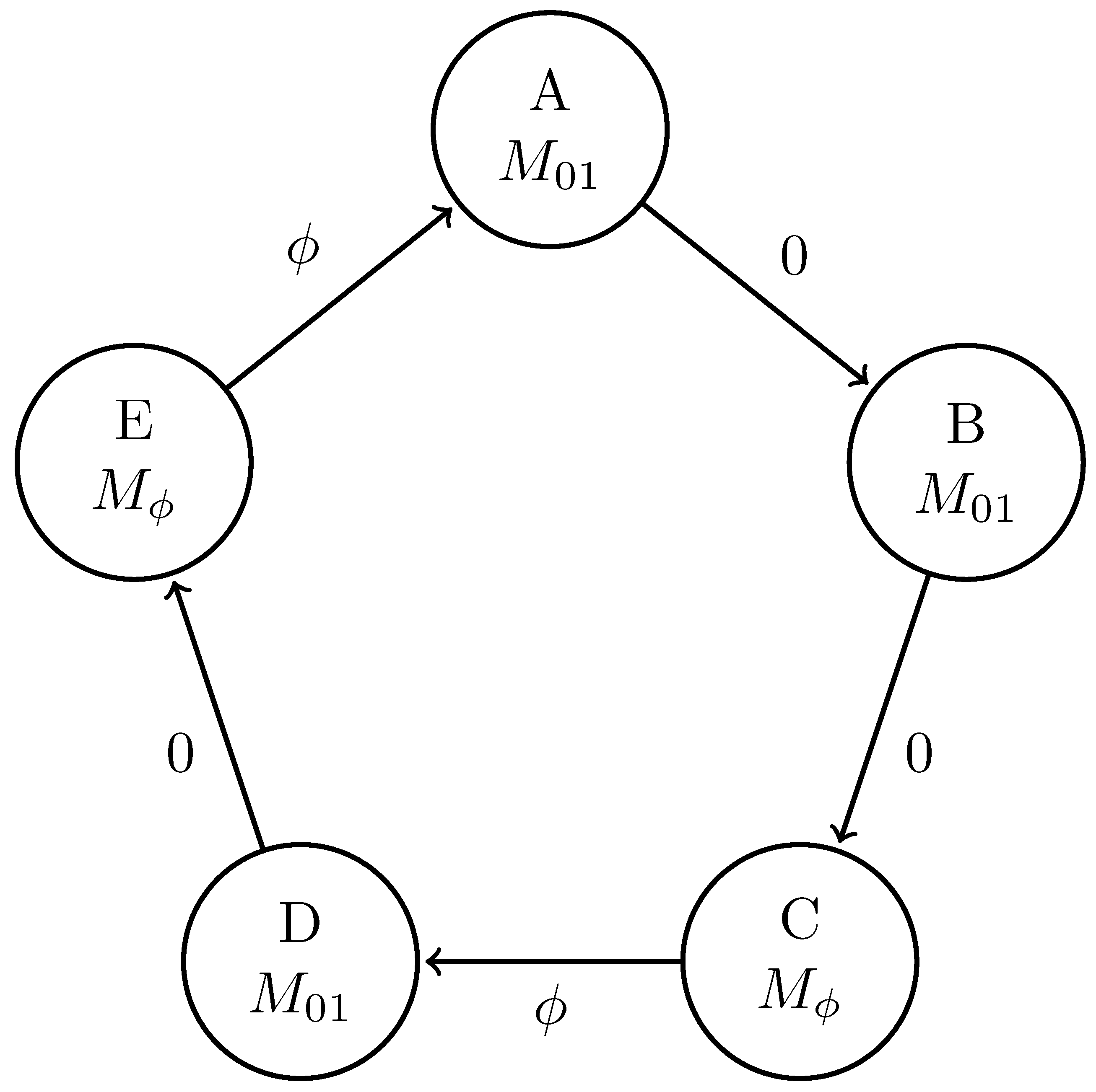
4.3. Periodic Processes
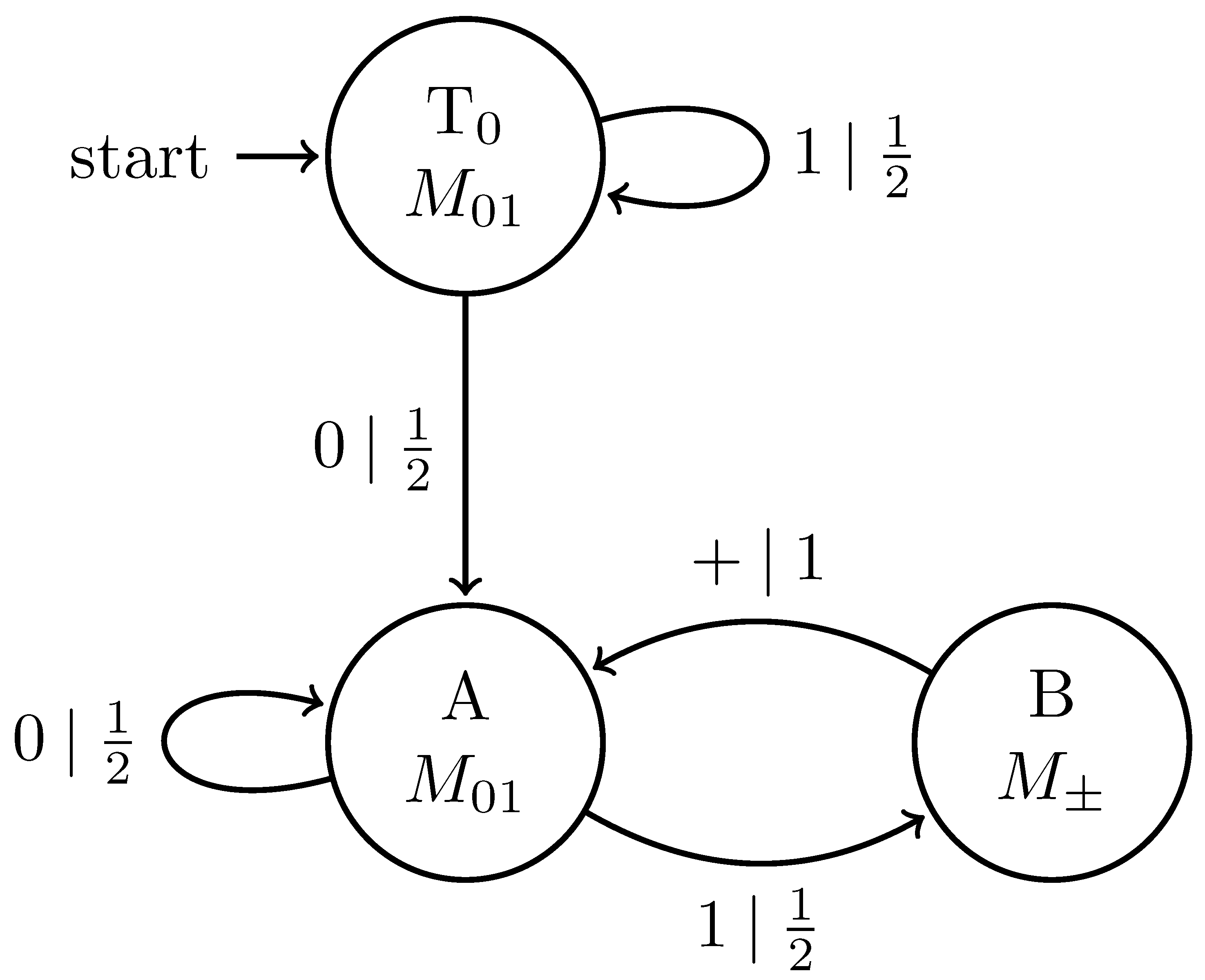
4.4. Quantum Golden Mean Processes
4.5. 3-Symbol Quantum Golden Mean
4.6. Unifilar and Nonunifilar Qubit Sources
4.7. Unifilar Qutrit Source
4.8. Discussion

| s | |||||
|---|---|---|---|---|---|
| (Bits/Time Step) | (Bits) | (Bits × Time Steps) | (Time Steps) | ||
| I.I.D. Qubit Process | 0 | 0 | 0 | ||
| Period-3 Process () | 0 | 1 | 3 | ||
| Period-3 Process () | 0 | 1 | ∞ | ||
| Quantum Golden Mean () | 1 | ||||
| Quantum Golden Mean () | 0.5505 | ∞ | |||
| 3-Symbol Quantum Golden Mean | 0.6667 | 0.3333 | ∞ | ||
| Unifilar Qubit Source () | 0.9184 | 0.0816 | ∞ | ||
| Nonunifilar Qubit Source () | 0.7306 | 0.2614 | ∞ | ||
| Unifilar Qutrit Source | 0.8002 | 0.7848 | ∞ | ||
5. Synchronizing to a Quantum Source
5.1. States of Knowledge
5.2. Average State Uncertainty and Synchronization Information
5.3. Synchronizing to Quantum Presentations of Classical Processes
5.4. Synchronizing to Periodic Processes
5.5. Synchronizing with PVMs
5.6. Maintaining Synchrony with Adaptive Measurement
5.7. Synchronizing to a Qutrit Source
5.8. Discussion
6. Quantum Process System Identification
6.1. Classical System Identification
6.2. Tomography of a Qudit
- ’s complete description requires a number of parameters that scales exponentially with the state’s Hilbert space dimension.
- Quantum measurement is probabilistic, so one must prepare and measure many copies of to estimate a single parameter.
6.3. Tomography of a Qudit Process
6.4. Cost of I.I.D.
6.5. Finite-Length Estimation of Information Properties
6.6. Tomography with a Known Quantum Alphabet
6.6.1.
6.6.2.
6.6.3.
6.7. Source Reconstruction
6.7.1.
6.7.2.
6.7.3.
6.8. Discussion
7. Conclusions
Author Contributions
Funding
Institutional Review Board Statement
Data Availability Statement
Acknowledgments
Conflicts of Interest
Appendix A. Information in Classical Processes
Appendix A.1. Shannon Entropy
Appendix A.2. Block Entropy
Appendix A.3. Shannon Entropy Rate
Appendix A.4. Redundancy
Appendix A.5. Block Entropy Derivatives and Integrals
Appendix A.6. Entropy Gain
Appendix A.7. Predictability Gain
Appendix A.8. Total Predictability
Appendix A.9. Excess Entropy
Appendix A.10. Transient Information
Appendix A.11. Markov Order
Appendix B. Quantum Channels for Preparation and Measurement
References
- Heisenberg, W. Über den anschaulichen inhalt der quantentheoretischen kinematik und mechanik. Z. Phys. 1927, 43, 172–198. [Google Scholar] [CrossRef]
- Peres, A. Two simple proofs of the Kochen-Specker theorem. J. Phys. A 1991, 24, L175. [Google Scholar] [CrossRef]
- Wootters, W.K.; Fields, B.D. Optimal state-determination by mutually unbiased measurements. Ann. Phys. 1989, 191, 363–381. [Google Scholar] [CrossRef]
- Renes, J.M.; Blume-Kohout, R.; Scott, A.J.; Caves, C.M. Symmetric informationally complete quantum measurements. J. Math. Phys. 2004, 45, 2171–2180. [Google Scholar] [CrossRef]
- von Neumann, J. Mathematical Foundations of Quantum Mechanics: New Edition; Princeton University Press: Princeton, NJ, USA, 2018. [Google Scholar]
- Wilde, M. Quantum Information Theory, 2nd ed.; Cambridge University Press: Cambridge, UK, 2017. [Google Scholar]
- Shannon, C.E. A mathematical theory of communication. Bell Sys. Tech. J. 1948, 27, 379–423+623–656. [Google Scholar] [CrossRef]
- Schumacher, B. Quantum coding. Phys. Rev. A 1995, 51, 2738–2747. [Google Scholar] [CrossRef]
- Crutchfield, J.P. Between order and chaos. Nat. Phys. 2012, 8, 17–24. [Google Scholar] [CrossRef]
- Crutchfield, J.P.; Young, K. Inferring statistical complexity. Phys. Rev. Let. 1989, 63, 105–108. [Google Scholar] [CrossRef]
- Crutchfield, J.P.; Feldman, D.P. Regularities unseen, randomness observed: Levels of entropy convergence. Chaos 2003, 13, 25–54. [Google Scholar] [CrossRef]
- Travers, N.F.; Crutchfield, J.P. Exact synchronization for finite-state sources. J. Stat. Phys. 2011, 145, 1181–1201. [Google Scholar] [CrossRef]
- Travers, N.F.; Crutchfield, J.P. Asymptotic synchronization for finite-state sources. J. Stat. Phys. 2011, 145, 1202–1223. [Google Scholar] [CrossRef]
- Venegas-Li, A.E.; Jurgens, A.M.; Crutchfield, J.P. Measurement-induced randomness and structure in controlled qubit processes. Phys. Rev. E 2020, 102, 040102. [Google Scholar] [CrossRef] [PubMed]
- Holevo, A.S. Quantum coding theorems. Usp. Mat. Nauk 1998, 53, 193–230. [Google Scholar] [CrossRef]
- Datta, N.; Suhov, Y. Data Compression Limit for an Information Source of Interacting Qubits. Quantum Inf. Process. 2002, 1, 257–281. [Google Scholar] [CrossRef]
- Petz, D.; Mosonyi, M. Stationary quantum source coding. J. Math. Phys. 2001, 42, 4857–4864. [Google Scholar] [CrossRef]
- Nagamatsu, Y.; Mizutani, A.; Ikuta, R.; Yamamoto, T.; Imoto, N.; Tamaki, K. Security of quantum key distribution with light sources that are not independently and identically distributed. Phys. Rev. A 2016, 93, 042325. [Google Scholar] [CrossRef]
- Pollock, F.A.; Rodriguez-Rosario, C.; Frauenheim, T.; Paternostro, M.; Modi, K. Operational Markov condition for quantum processes. Phys. Rev. Lett. 2018, 120, 040405. [Google Scholar] [CrossRef]
- Pollock, F.A.; Rodriguez-Rosario, C.; Frauenheim, T.; Paternostro, M.; Modi, K. Non-Markovian quantum processes: Complete framework and efficient characterization. Phys. Rev. A 2018, 97, 012127. [Google Scholar] [CrossRef]
- Taranto, P.; Pollock, F.A.; Milz, S.; Tomamichel, M.; Modi, K. Quantum Markov order. Phys. Rev. Lett. 2019, 122, 14041. [Google Scholar] [CrossRef]
- Taranto, P.; Pollock, F.A.; Modi, K. Non-Markovian memory strength bounds quantum process recoverability. npj Quantum Inf. 2021, 7, 149. [Google Scholar] [CrossRef]
- Taranto, P.; Milz, S.; Pollock, F.A.; Modi, K. Structure of quantum stochastic processes with finite Markov order. Phys. Rev. A 2019, 99, 042108. [Google Scholar] [CrossRef]
- Schon, C.; Solano, E.; Verstraete, F.; Cirac, J.I.; Wolf, M.M. Sequential generation of entangled multiqubit states. Phys. Rev. Lett. 2005, 95, 110503. [Google Scholar] [CrossRef]
- Schon, C.; Hammerer, K.; Wolf, M.M.; Cirac, J.O.; Solano, E. Sequential generation of matrix-product states in cavity QED. Phys. Rev. A 2007, 55, 032311. [Google Scholar] [CrossRef]
- Boyd, A.B.; Mandal, D.; Crutchfield, J.P. Correlation-powered information engines and the thermodynamics of self-correction. Phys. Rev. E 2017, 95, 012152. [Google Scholar] [CrossRef]
- Chapman, A.; Miyake, A. How an autonomous quantum Maxwell demon can harness correlated information. Phys. Rev. E 2015, 92, 062125. [Google Scholar] [CrossRef] [PubMed]
- Gu, M.; Wiesner, K.; Rieper, E.; Vedral, V. Occam’s quantum razor: How quantum mechanics can reduce the complexity of classical models. Nat. Commun. 2012, 3, 762. [Google Scholar] [CrossRef]
- Mahoney, J.R.; Aghamohammadi, C.; Crutchfield, J.P. Occam’s quantum strop: Synchronizing and compressing classical cryptic processes via a quantum channel. Sci. Rep. 2016, 6, 20495. [Google Scholar] [CrossRef] [PubMed]
- Suen, W.Y.; Elliot, T.J.; Thompson, J.; Garner, A.J.; Mahoney, J.R.; Vedral, V.; Gu, M. Surveying structural complexity in quantum many-body systems. J. Stat. Phys. 2022, 187, 4. [Google Scholar] [CrossRef]
- Binder, F.C.; Thompson, J.; Gu, M. Practical unitary simulator for non-Markovian complex processes. Phys. Rev. Lett. 2018, 120, 240502. [Google Scholar] [CrossRef]
- Loomis, S.P.; Crutchfield, J.P. Strong and Weak Optimizations in Classical and Quantum Models of Stochastic Processes. J. Stat. Phys. 2019, 176, 1317–1342. [Google Scholar] [CrossRef]
- Nielsen, M.A.; Chuang, I.L. Quantum Computation and Quantum Information: 10th Anniversary Edition, 10th ed.; Cambridge University Press: Cambridge, MA, USA, 2011. [Google Scholar]
- Gudder, S. Quantum Markov chains. J. Math. Phys. 2008, 49, 072105. [Google Scholar] [CrossRef]
- Monras, A.; Beige, A.; Wiesner, K. Hidden Quantum Markov Models and non-adaptive read-out of many-body states. arXiv 2010, arXiv:1002.2337. [Google Scholar]
- Wiesner, K.; Crutchfield, J.P. Computation in finitary stochastic and quantum processes. Phys. D 2008, 237, 1173–1195. [Google Scholar] [CrossRef]
- Srinivasan, S.; Gordon, G.; Boots, B. Learning hidden quantum Markov models. In Proceedings of the International Conference on Artificial Intelligence and Statistics, Playa Blanca, Spain, 9–11 April 2018; pp. 1979–1987. [Google Scholar]
- Perez-Garcia, D.; Verstraete, F.; Wolf, M.M.; Cirac, J.I. Matrix product state representations. arXiv 2006, arXiv:quant-ph/0608197. [Google Scholar] [CrossRef]
- Verstraete, F.; García-Ripoll, J.J.; Cirac, J.I. Matrix product density operators: Simulation of finite-temperature and dissipative systems. Phys. Rev. Lett. 2004, 93, 207204. [Google Scholar] [CrossRef]
- Moore, C.; Crutchfield, J.P. Quantum automata and quantum grammars. Theoret. Comp. Sci. 2000, 237, 275–306. [Google Scholar] [CrossRef]
- Qiu, D.; Li, L.; Mateus, P.; Gruska, J. Quantum Finite Automata. In Handbook of Finite State Based Models and Applications; CRC Press: Boca Raton, FL, USA, 2012; Volume 10, pp. 113–144. [Google Scholar]
- Zheng, S.; Qiu, D.; Li, L.; Gruska, J. One-way finite automata with quantum and classical states. In Lecture Notes in Computer Science; Springer: Berlin/Heidelberg, Germany, 2012; Volume 7300, pp. 273–290. [Google Scholar]
- Junge, M.; Renner, R.; Sutter, D.; Wilde, M.M.; Winter, A. Universal recovery maps and approximate sufficiency of quantum relative entropy. Ann. Henri Poincaré 2018, 19, 2955–2978. [Google Scholar] [CrossRef]
- Lanford, O.E.; Robinson, D.W. Mean entropy of states in quantum-statistical mechanics. J. Math. Phys. 1968, 9, 1120–1125. [Google Scholar] [CrossRef]
- Ohya, M.; Petz, D. Quantum Entropy and Its Use; Springer: Berlin/Heidelberg, Germany, 1993. [Google Scholar]
- Cover, T.M.; Thomas, J.A. Elements of Information Theory; Wiley-Interscience: New York, NY, USA, 1991. [Google Scholar]
- Travers, N.F.; Crutchfield, J.P. Equivalence of history and generator ϵ-machines. arXiv 2011, arXiv:1111.4500. [Google Scholar]
- Ellison, C.J.; Mahoney, J.R.; Crutchfield, J.P. Prediction, retrodiction, and the amount of information stored in the present. J. Stat. Phys. 2009, 136, 1005–1034. [Google Scholar] [CrossRef]
- Jurgens, A.M.; Crutchfield, J.P. Shannon entropy rate of hidden Markov processes. J. Stat. Phys. 2021, 183, 32. [Google Scholar] [CrossRef]
- Crutchfield, J.P.; Riechers, P.; Ellison, C.J. Exact complexity: Spectral decomposition of intrinsic computation. Phys. Lett. A 2016, 380, 998–1002. [Google Scholar] [CrossRef]
- Marzen, S.; Crutchfield, J.P. Informational and causal architecture of discrete-time renewal processes. Entropy 2015, 17, 4891–4917. [Google Scholar] [CrossRef]
- Jurgens, A.; Crutchfield, J.P. Divergent predictive states: The statistical complexity dimension of stationary, ergodic hidden Markov processes. Chaos 2021, 31, 0050460. [Google Scholar] [CrossRef]
- Fujiwara, Y. Parsing a sequence of qubits. IEEE Trans. Inf. Theory 2013, 59, 6796–6806. [Google Scholar] [CrossRef]
- Strelioff, C.C.; Crutchfield, J.P. Bayesian structural inference for hidden processes. Phys. Rev. E 2014, 89, 042119. [Google Scholar] [CrossRef] [PubMed]
- Thew, R.T.; Nemoto, K.; White, A.G.; Munro, W.J. Qudit quantum-state tomography. Phys. Rev. A 2002, 66, 012303. [Google Scholar] [CrossRef]
- Bengtsson, I.; Życzkowski, K. Geometry of Quantum States: An Introduction to Quantum entanglement; Cambridge University Press: Cambridge, UK, 2017. [Google Scholar]
- Lawrence, J.; Brukner, Č.; Zeilinger, A. Mutually unbiased binary observable sets on n qubits. Phys. Rev. A 2002, 65, 032320. [Google Scholar] [CrossRef]
- Gharibian, S. Strong NP-hardness of the quantum separability problem. arXiv 2008, arXiv:0810.4507. [Google Scholar] [CrossRef]
- Horodecki, P. Separability criterion and inseparable mixed states with positive partial transposition. Phys. Lett. A 1997, 232, 333–339. [Google Scholar] [CrossRef]
- Horodecki, M.; Horodecki, P.; Horodecki, R. Separability of n-particle mixed states: Necessary and sufficient conditions in terms of linear maps. Phys. Lett. A 2001, 283, 1–7. [Google Scholar] [CrossRef]
- Pirvu, B.; Murg, V.; Cirac, J.I.; Verstraete, F. Matrix product operator representations. New J. Phys. 2010, 12, 025012. [Google Scholar] [CrossRef]
- Riechers, P.; Crutchfield, J.P. Spectral simplicity of apparent complexity, Part I: The nondiagonalizable metadynamics of prediction. Chaos 2018, 28, 033115. [Google Scholar] [CrossRef] [PubMed]
- Riechers, P.M.; Crutchfield, J.P. Beyond the spectral theorem: Decomposing arbitrary functions of nondiagonalizable operators. AIP Adv. 2018, 8, 065305. [Google Scholar] [CrossRef]
- Riechers, P.; Crutchfield, J.P. Spectral simplicity of apparent complexity, Part II: Exact complexities and complexity spectra. Chaos 2018, 28, 033116. [Google Scholar] [CrossRef]
- Shalizi, C.R.; Crutchfield, J.P. Computational mechanics: Pattern and prediction, structure and simplicity. J. Stat. Phys. 2001, 104, 817–879. [Google Scholar] [CrossRef]
- Landauer, R. Irreversibility and heat generation in the computing process. IBM J. Res. Dev. 1961, 5, 183–191. [Google Scholar] [CrossRef]
- Boyd, A.B.; Mandal, D.; Crutchfield, J.P. Leveraging environmental correlations: The thermodynamics of requisite variety. J. Stat. Phys. 2016, 167, 1555–1585. [Google Scholar] [CrossRef]
- Jurgens, A.M.; Crutchfield, J.P. Functional thermodynamics of Maxwellian ratchets: Constructing and deconstructing patterns, randomizing and derandomizing behaviors. Phys. Rev. Res. 2020, 2, 033334. [Google Scholar] [CrossRef]
- Huang, R.; Riechers, P.; Gu, M.; Narasimhachar, V. Engines for predictive work extraction from memoryfull quantum stochastic processes. arXiv 2022, arXiv:2207.03480v5. [Google Scholar]
- Cover, T.M.; Thomas, J.A. Elements of Information Theory, 2nd ed.; Wiley-Interscience: New York, NY, USA, 2006. [Google Scholar]
- James, R.G.; Mahoney, J.R.; Ellison, C.J.; Crutchfield, J.P. Many roads to synchrony: Natural time scales and their algorithms. Phys. Rev. E 2014, 89, 042135. [Google Scholar] [CrossRef] [PubMed]
- Travers, N.F. Exponential bounds for convergence of entropy rate approximations in hidden Markov models satisfying a path-mergeability condition. Stoch. Proc. Appl. 2014, 124, 4149–4170. [Google Scholar] [CrossRef]


Disclaimer/Publisher’s Note: The statements, opinions and data contained in all publications are solely those of the individual author(s) and contributor(s) and not of MDPI and/or the editor(s). MDPI and/or the editor(s) disclaim responsibility for any injury to people or property resulting from any ideas, methods, instructions or products referred to in the content. |
© 2025 by the authors. Licensee MDPI, Basel, Switzerland. This article is an open access article distributed under the terms and conditions of the Creative Commons Attribution (CC BY) license (https://creativecommons.org/licenses/by/4.0/).
Share and Cite
Gier, D.; Crutchfield, J.P. Intrinsic and Measured Information in Separable Quantum Processes. Entropy 2025, 27, 599. https://doi.org/10.3390/e27060599
Gier D, Crutchfield JP. Intrinsic and Measured Information in Separable Quantum Processes. Entropy. 2025; 27(6):599. https://doi.org/10.3390/e27060599
Chicago/Turabian StyleGier, David, and James P. Crutchfield. 2025. "Intrinsic and Measured Information in Separable Quantum Processes" Entropy 27, no. 6: 599. https://doi.org/10.3390/e27060599
APA StyleGier, D., & Crutchfield, J. P. (2025). Intrinsic and Measured Information in Separable Quantum Processes. Entropy, 27(6), 599. https://doi.org/10.3390/e27060599