
Information-Theoretic Reliability Analysis of Linear Consecutive r-out-of-n:F Systems and Uniformity Testing


Abstract
1. Introduction
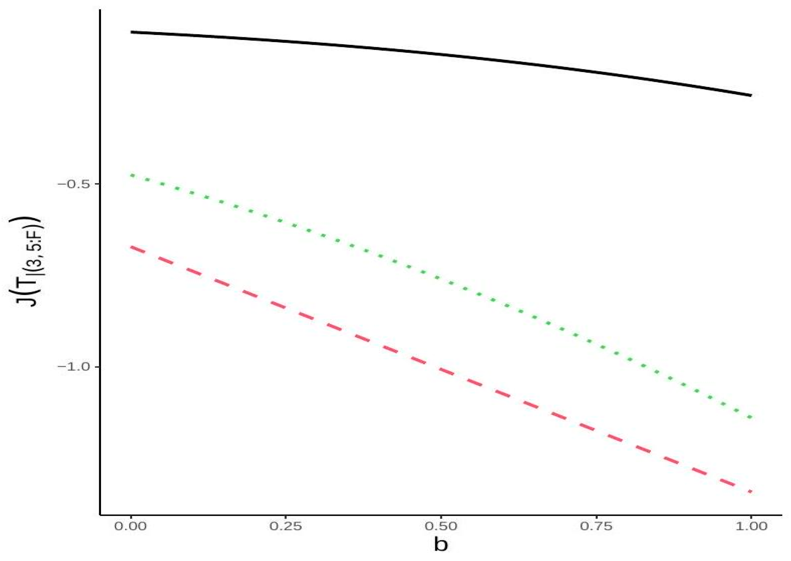
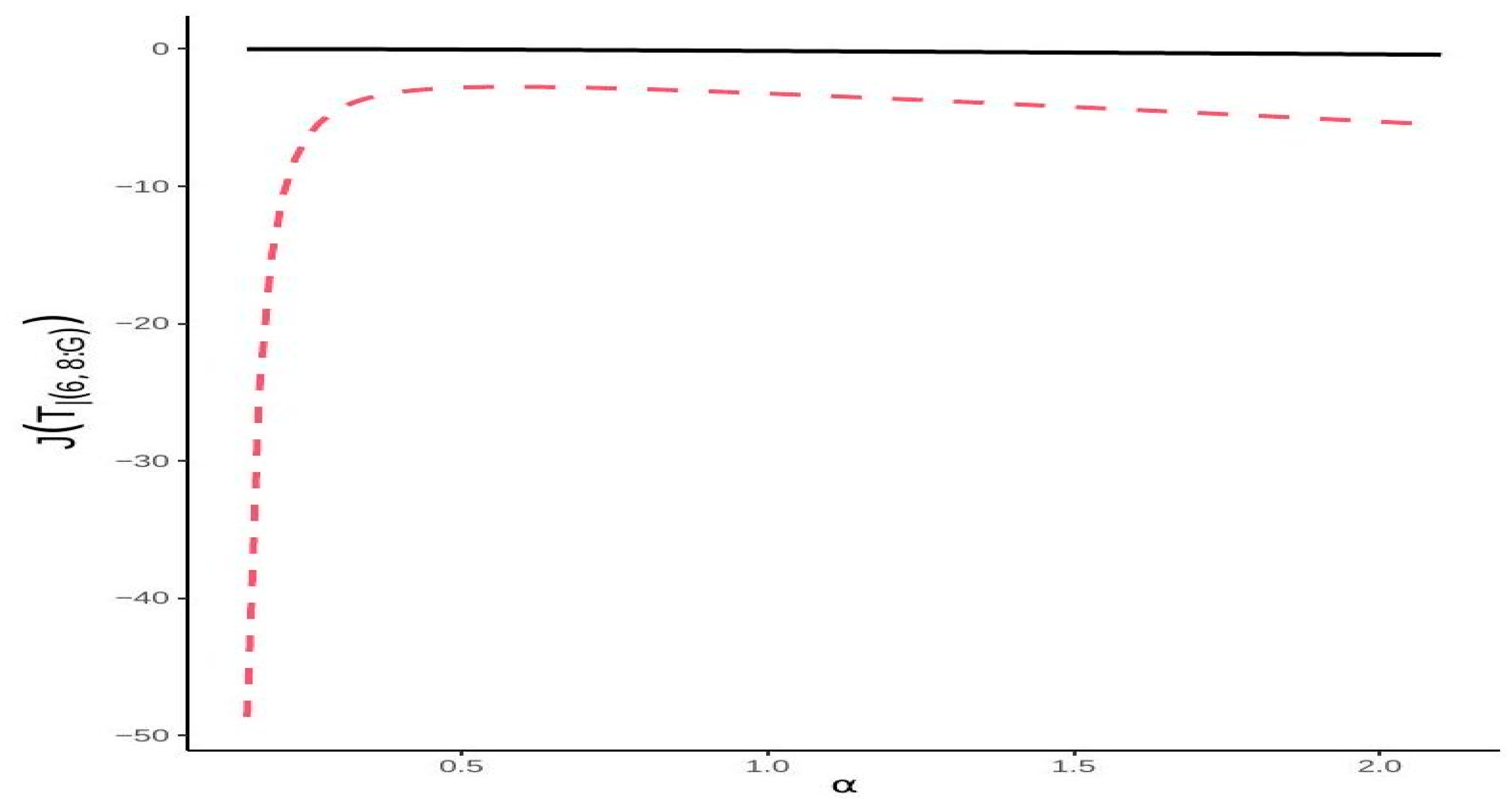
2. Extropy of Consecutive -out-of-:F System
3. Bounds of Extropy of Consecutive Systems
- (i)
- If , where designates the mode of the pdf , for , we have .
- (ii)
- For , we have
4. Characterization Results
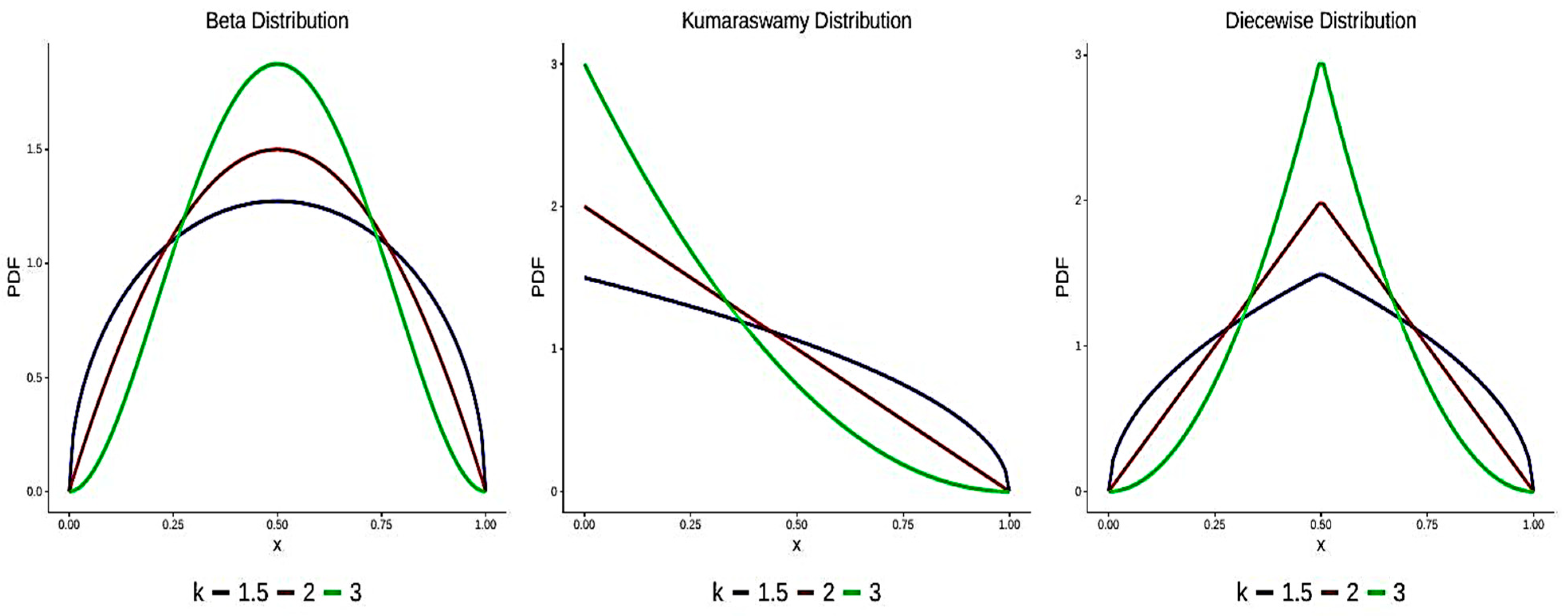
5. Nonparametric Estimation
5.1. Test of Uniformity
- (i)
- ,
- (ii)
- ,
- (iii)
- .
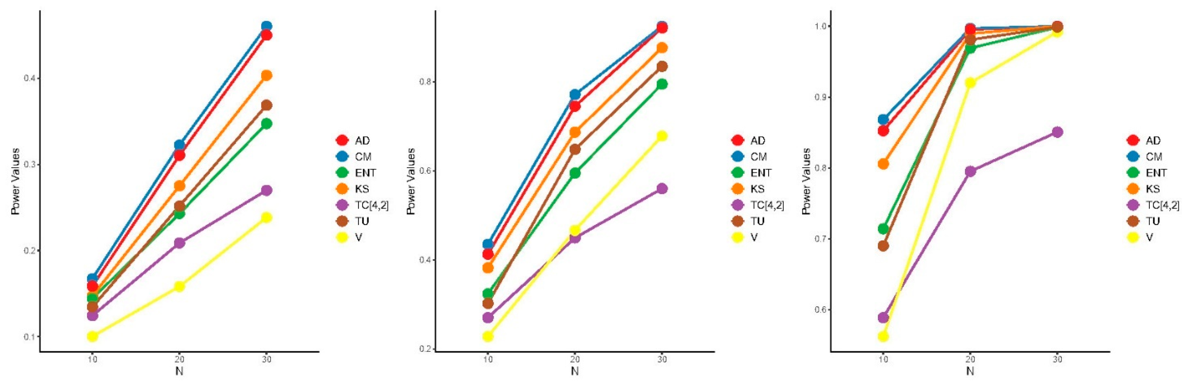
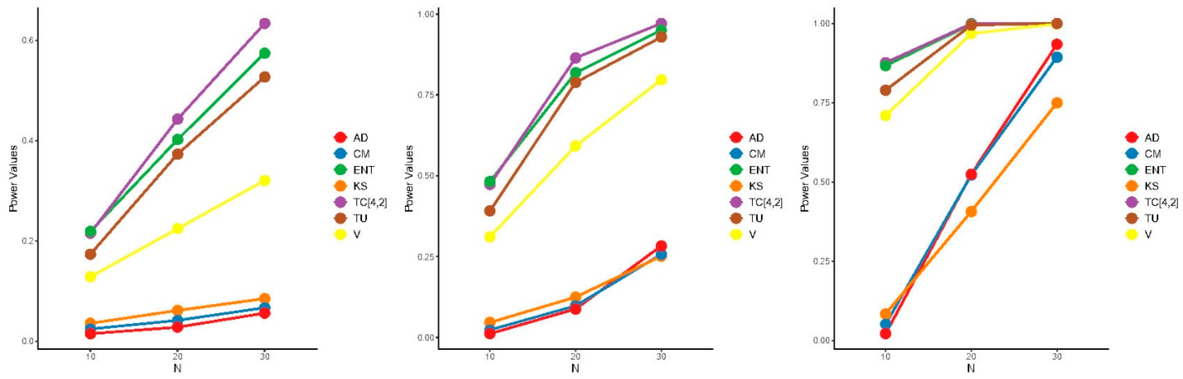
5.2. Power Comparisons
- ,
- ,
- for , where
6. Conclusions
Author Contributions
Funding
Institutional Review Board Statement
Data Availability Statement
Acknowledgments
Conflicts of Interest
References
- Shannon, C.E. A mathematical theory of communication. Bell Syst. Tech. J. 1948, 27, 379–423. [Google Scholar]
- Lad, F.; Sanfilippo, G.; Agro, G. Extropy: Complementary dual of entropy. Stat. Sci. 2015, 30, 40–58. [Google Scholar] [CrossRef]
- Agro, G.; Lad, F.; Sanfilippo, G. Sequentially forecasting economic indices using mixture linear combinations of EP distributions. J. Data Sci. 2010, 8, 101–126. [Google Scholar] [CrossRef]
- Capotorti, A.; Regoli, G.; Vattari, F. Correction of incoherent conditional probability assessments. Int. J. Approx. Reason. 2010, 51, 718–727. [Google Scholar] [CrossRef]
- Gneiting, T.; Raftery, A.E. Strictly proper scoring rules, prediction, and estimation. J. Am. Stat. Assoc. 2007, 102, 359–378. [Google Scholar] [CrossRef]
- Toomaj, A.; Hashempour, M.; Balakrishnan, N. Extropy: Characterizations and dynamic versions. J. Appl. Probab. 2023, 60, 1333–1351. [Google Scholar] [CrossRef]
- Yang, J.; Xia, W.; Hu, T. Bounds on extropy with variational distance constraint. Probab. Eng. Informational Sci. 2019, 33, 186–204. [Google Scholar] [CrossRef]
- Jung, K.-H.; Kim, H. Linear consecutive-k-out-of-n: F system reliability with common-mode forced outages. Reliab. Eng. Syst. Saf. 1993, 41, 49–55. [Google Scholar] [CrossRef]
- Shen, J.; Zuo, M.J. Optimal design of series consecutive-k-out-of-n: G systems. Reliab. Eng. Syst. Saf. 1994, 45, 277–283. [Google Scholar] [CrossRef]
- Kuo, W.; Zuo, M.J. Optimal Reliability Modeling: Principles and Applications; John Wiley and Sons: Hoboken, NJ, USA, 2003. [Google Scholar]
- In-Hang, C.; Cui, L.; Hwang, F.K. Reliabilities of Consecutive-k Systems; Springer Nature: Berlin/Heidelberg, Germany, 2013. [Google Scholar]
- Boland, P.J.; Samaniego, F.J. Stochastic ordering results for consecutive k-out-of-n: F systems. IEEE Trans. Reliab. 2004, 53, 7–10. [Google Scholar] [CrossRef]
- Eryılmaz, S. Mixture representations for the reliability of consecutive-k systems. Math. Comput. Model. 2010, 51, 405–412. [Google Scholar] [CrossRef]
- Eryilmaz, S. Conditional lifetimes of consecutive k-out-of-n systems. IEEE Trans. Reliab. 2010, 59, 178–182. [Google Scholar] [CrossRef]
- Wong, K.M.; Chen, S. The entropy of ordered sequences and order statistics. IEEE Trans. Inf. Theory 1990, 36, 276–284. [Google Scholar] [CrossRef]
- Park, S. The entropy of consecutive order statistics. IEEE Trans. Inf. Theory 1995, 41, 2003–2007. [Google Scholar] [CrossRef]
- Ebrahimi, N.; Soofi, E.S.; Soyer, R. Information measures in perspective. Int. Stat. Rev. 2010, 78, 383–412. [Google Scholar] [CrossRef]
- Zarezadeh, S.; Asadi, M. Results on residual Rényi entropy of order statistics and record values. Inf. Sci. 2010, 180, 4195–4206. [Google Scholar] [CrossRef]
- Baratpour, S.; Ahmadi, J.; Arghami, N.R. Characterizations based on Rényi entropy of order statistics and record values. J. Stat. Plan. Inference 2008, 138, 2544–2551. [Google Scholar] [CrossRef]
- Qiu, G. The extropy of order statistics and record values. Stat. Probab. Lett. 2017, 120, 52–60. [Google Scholar] [CrossRef]
- Qiu, G.; Jia, K. Extropy estimators with applications in testing uniformity. J. Nonparametric Stat. 2018, 30, 182–196. [Google Scholar] [CrossRef]
- Qiu, G.; Jia, K. The residual extropy of order statistics. Stat. Probab. Lett. 2018, 133, 15–22. [Google Scholar] [CrossRef]
- Kayid, M.; Alshehri, M.A. System level extropy of the past life of a coherent system. J. Math. 2023, 2013, 9912509. [Google Scholar] [CrossRef]
- Shrahili, M.; Kayid, M. Excess lifetime extropy of order statistics. Axioms 2023, 12, 1024. [Google Scholar] [CrossRef]
- Shrahili, M.; Kayid, M.; Mesfioui, M. Stochastic inequalities involving past extropy of order statistics and past extropy of record values. AIMS Math. 2024, 9, 5827–5849. [Google Scholar] [CrossRef]
- Kayid, M.; Alshehri, M.A. Excess lifetime extropy for a mixed system at the system level. AIMS Math 2023, 8, 16137–16150. [Google Scholar] [CrossRef]
- Alrewely, F.; Kayid, M. Extropy analysis in consecutive r-out-of-n: G systems with applications in reliability and exponentiality testing. AIMS Math. 2025, 10, 6040–6068. [Google Scholar] [CrossRef]
- Navarro, J.; Eryilmaz, S. Mean residual lifetimes of consecutive-k-out-of-n systems. J. Appl. Probab. 2007, 44, 82–98. [Google Scholar] [CrossRef]
- Shaked, M.; Shanthikumar, J.G. Stochastic Orders; Springer Science and Business Media: Berlin/Heidelberg, Germany, 2007. [Google Scholar]
- Bagai, I.; Kochar, S.C. On tail-ordering and comparison of failure rates. Commun. Stat. Theory Methods 1986, 15, 1377–1388. [Google Scholar] [CrossRef]
- Husseiny, I.A.; Barakat, H.M.; Nagy, M.; Mansi, A.H. Analyzing symmetric distributions by utilizing extropy measures based on order statistics. J. Radiat. Res. Appl. Sci. 2024, 17, 101100. [Google Scholar] [CrossRef]
- Gupta, N.; Chaudhary, S.K. Some characterizations of continuous symmetric distributions based on extropy of record values. Stat. Pap. 2024, 65, 291–308. [Google Scholar] [CrossRef]
- Kamps, U. 10 characterizations of distributions by recurrence relations and identities for moments of order statistics. In Handbook of Statistics; Confederation of Indian Industry: New Delhi, India, 1998; Volume 16, pp. 291–311. [Google Scholar]
- Hwang, J.S.; Lin, G.D. On a generalized moment problem. II. Proc. Am. Math. Soc. 1984, 91, 577–580. [Google Scholar] [CrossRef]
- Vasicek, O. A test for normality based on sample entropy. J. R. Stat. Soc. Ser. B: Stat. Methodol. 1976, 38, 54–59. [Google Scholar] [CrossRef]
- Crzcgorzewski, P.; Wirczorkowski, R. Entropy-based goodness-of-fit test for exponentiality. Commun. Stat. Theory Methods 1999, 28, 1183–1202. [Google Scholar] [CrossRef]
- Park, S. A goodness-of-fit test for normality based on the sample entropy of order statistics. Stat. Probab. Lett. 1999, 44, 359–363. [Google Scholar] [CrossRef]
- Xiong, P.; Zhuang, W.; Qiu, G. Testing exponentiality based on the extropy of record values. J. Appl. Stat. 2022, 49, 782–802. [Google Scholar] [CrossRef]
- Ebrahimi, N.; Pflughoeft, K.; Soofi, E.S. Two measures of sample entropy. Stat. Probab. Lett. 1994, 20, 225–234. [Google Scholar] [CrossRef]
- Cordeiro, G.M.; De Castro, M. A new family of generalized distributions. J. Stat. Comput. Simul. 2011, 81, 883–898. [Google Scholar] [CrossRef]
- Kolmogorov, A.N. Sulla determinazione empirica di una legge di distribuzione. Giorn. Dell’Inst. Ital. Degli Atti 1933, 4, 89–91. [Google Scholar]
- Smirnov, N.V. Estimate of deviation between empirical distribution functions in two independent samples. Bull. Mosc. Univ. 1939, 2, 3–16. [Google Scholar]
- American Statistical Association. Journal of the American Statistical Association; American Statistical Association: Alexandria, VA, USA, 1922. [Google Scholar]
- Cramér, H. On the Composition of Elementary Errors: Statistical Applications; Almqvist and Wiksell: Stockholm, Sweden, 1928. [Google Scholar]
- Mises, R. Wahrscheinlichkeitsrechnung und ihre Anwendung in der Statistik und theoretischen Physik; Rosenberg, M.S., Ed.; F. Deuticke: Vienna, Austria, 1931. [Google Scholar]
- Illowsky, B.; Dean, S. Introductory Statistics; OpenStax: Houston, TX, USA, 2018. [Google Scholar]
- Tahmasebi, S.; Toomaj, A. On negative cumulative extropy with applications. Commun. Stat. Theory Methods 2022, 51, 5025–5047. [Google Scholar] [CrossRef]
- Balakrishnan, N.; Buono, F.; Longobardi, M. On Tsallis extropy with an application to pattern recognition. Stat. Probab. Lett. 2022, 180, 109241. [Google Scholar] [CrossRef]
- Kazemi, M.R.; Tahmasebi, S.; Buono, F.; Longobardi, M. Fractional Deng entropy and extropy and some applications. Entropy 2021, 23, 623. [Google Scholar] [CrossRef] [PubMed]
- Tahmasebi, S.; Kazemi, M.R.; Keshavarz, A.; Jafari, A.A.; Buono, F. Compressive sensing using extropy measures of ranked set sampling. Math. Slovaca 2023, 73, 245–262. [Google Scholar]
- Blinov, P.Y.; Lemeshko, B.Y. A review of the properties of tests for uniformity. In Proceedings of the 2014 12th International Conference on Actual Problems of Electronic Instrument Engineering, Novosibirsk, Russia, 2–4 October 2014. [Google Scholar]
- Mohamed, M.S.; Barakat, H.M.; Alyami, S.A.; Abd Elgawad, M.A. Fractional entropy-based test of uniformity with power comparisons. J. Math. 2021, 2021, 5331260. [Google Scholar] [CrossRef]
- Mohamed, M.S.; Barakat, H.M.; Alyami, S.A.; Abd Elgawad, M.A. Cumulative residual Tsallis entropy-based test of uniformity and some new findings. Mathematics 2022, 10, 771. [Google Scholar] [CrossRef]
- Noughabi, H.A. Cumulative residual entropy applied to testing uniformity. Commun. Stat. Theory Methods 2022, 51, 4151–4161. [Google Scholar] [CrossRef]


| N = 20 | N = 30 | N = 40 | N = 50 | N = 100 | |||||||
|---|---|---|---|---|---|---|---|---|---|---|---|
| n | i | Bias | RMSE | Bias | RMSE | Bias | RMSE | Bias | RMSE | Bias | RMSE |
| 5 | 0 | −0.145895 | 0.050749 | −0.089774 | 0.018277 | −0.059770 | 0.009551 | −0.044811 | 0.005837 | −0.011864 | 0.001097 |
| 1 | −0.078625 | 0.018531 | −0.041885 | 0.006271 | −0.026529 | 0.003121 | −0.017465 | 0.001909 | −0.003345 | 0.000571 | |
| 2 | −0.036039 | 0.006134 | −0.018140 | 0.003219 | −0.012438 | 0.002164 | −0.009271 | 0.001516 | −0.004116 | 0.000757 | |
| 6 | 0 | −0.177926 | 0.071332 | −0.111349 | 0.028405 | −0.083625 | 0.015152 | −0.064254 | 0.009374 | −0.020052 | 0.001779 |
| 1 | −0.118696 | 0.031228 | −0.066450 | 0.011488 | −0.041432 | 0.005272 | −0.029434 | 0.003241 | −0.006391 | 0.000766 | |
| 2 | −0.055588 | 0.011645 | −0.026799 | 0.003965 | −0.015054 | 0.002124 | −0.009608 | 0.001451 | −0.000843 | 0.000593 | |
| 3 | −0.028573 | 0.007610 | −0.019522 | 0.004667 | −0.014865 | 0.003251 | −0.009383 | 0.002604 | −0.007302 | 0.001241 | |
| 7 | 0 | −0.215926 | 0.105451 | −0.143378 | 0.041398 | −0.105595 | 0.022722 | −0.083527 | 0.015081 | −0.027646 | 0.002861 |
| 1 | −0.151213 | 0.053749 | −0.089206 | 0.020752 | −0.061046 | 0.010124 | −0.044897 | 0.006181 | −0.011651 | 0.001151 | |
| 2 | −0.087616 | 0.021155 | −0.045373 | 0.007131 | −0.026959 | 0.003476 | −0.017064 | 0.002072 | −0.001945 | 0.000608 | |
| 3 | −0.037821 | 0.008069 | −0.016963 | 0.003372 | −0.008987 | 0.002098 | −0.003187 | 0.001562 | −0.000514 | 0.000770 | |
| 8 | 0 | −0.245875 | 0.133512 | −0.169920 | 0.058762 | −0.127069 | 0.031831 | −0.101061 | 0.021011 | −0.038070 | 0.004022 |
| 1 | −0.188737 | 0.081671 | −0.116732 | 0.032998 | −0.084663 | 0.016489 | −0.063760 | 0.010117 | −0.018165 | 0.001815 | |
| 2 | −0.124965 | 0.036731 | −0.068022 | 0.013715 | −0.042473 | 0.006675 | −0.031082 | 0.003656 | −0.004798 | 0.000838 | |
| 3 | −0.065324 | 0.015026 | −0.028932 | 0.005053 | −0.014906 | 0.002663 | −0.007793 | 0.001549 | 0.001065 | 0.000666 | |
| 4 | −0.024499 | 0.008091 | −0.011365 | 0.003940 | −0.005889 | 0.002853 | −0.001748 | 0.002046 | −0.002914 | 0.001145 | |
| N = 20 | N = 30 | N = 40 | N = 50 | N = 100 | |||||||
|---|---|---|---|---|---|---|---|---|---|---|---|
| n | i | Bias | RMSE | Bias | RMSE | Bias | RMSE | Bias | RMSE | Bias | RMSE |
| 5 | 0 | −0.936094 | 1.444092 | −0.793851 | 1.144772 | −0.713842 | 1.004388 | −0.664756 | 0.905735 | −0.512761 | 0.628195 |
| 1 | −0.590450 | 0.871130 | −0.454252 | 0.658060 | −0.386377 | 0.536204 | −0.344834 | 0.463333 | −0.238968 | 0.311527 | |
| 2 | −0.260561 | 0.347903 | −0.188247 | 0.236120 | −0.147586 | 0.187416 | −0.124121 | 0.159152 | −0.075071 | 0.097070 | |
| 6 | 0 | −1.115787 | 1.785087 | −0.966685 | 1.404569 | −0.898500 | 1.260244 | −0.849516 | 1.141714 | −0.655093 | 0.859432 |
| 1 | −0.789329 | 1.243988 | −0.640423 | 0.918773 | −0.574205 | 0.796915 | −0.527410 | 0.702302 | −0.369448 | 0.471387 | |
| 2 | −0.461131 | 0.652054 | −0.335695 | 0.465028 | −0.276477 | 0.379773 | −0.235081 | 0.320505 | −0.152461 | 0.199439 | |
| 3 | −0.195613 | 0.259936 | −0.131979 | 0.179150 | −0.101657 | 0.142935 | −0.082456 | 0.119049 | −0.048043 | 0.078041 | |
| 7 | 0 | −1.300057 | 2.517281 | −1.340618 | 2.220741 | −1.390172 | 2.041344 | −1.351307 | 1.832077 | −1.174914 | 1.460273 |
| 1 | −0.974527 | 1.521404 | −0.835748 | 1.250773 | −0.752920 | 1.064358 | −0.703541 | 0.932074 | −0.515872 | 0.670624 | |
| 2 | −0.663265 | 0.980888 | −0.519456 | 0.705243 | −0.435916 | 0.605943 | −0.388588 | 0.509926 | −0.257060 | 0.332286 | |
| 3 | −0.347348 | 0.489964 | −0.246278 | 0.340897 | −0.191480 | 0.257628 | −0.155908 | 0.216469 | −0.094337 | 0.130185 | |
| 8 | 0 | −1.280009 | 2.387094 | −1.292371 | 1.970096 | −1.220243 | 1.730366 | −1.173613 | 1.614975 | −0.998048 | 1.256077 |
| 1 | −1.149068 | 1.823176 | −1.009816 | 1.512126 | −0.934285 | 1.290326 | −0.866499 | 1.153410 | −0.657747 | 0.844607 | |
| 2 | −0.864234 | 1.323735 | −0.723328 | 0.999044 | −0.611858 | 0.838130 | −0.560017 | 0.738741 | −0.393868 | 0.510655 | |
| 3 | −0.583059 | 0.817869 | −0.411258 | 0.576096 | −0.329835 | 0.453799 | −0.285657 | 0.389149 | −0.176501 | 0.234242 | |
| 4 | −0.283538 | 0.391618 | −0.192602 | 0.260096 | −0.139642 | 0.198825 | −0.111210 | 0.170093 | −0.061858 | 0.107112 | |
| m | N = 5 | N = 10 | N = 20 | N = 30 | N = 40 | N = 50 | N = 100 |
|---|---|---|---|---|---|---|---|
| 2 | 1.055246 | 0.378625 | 0.334115 | 0.292918 | 0.235903 | 0.214288 | 0.145114 |
| 3 | 0.291554 | 0.230632 | 0.203458 | 0.181164 | 0.164139 | 0.111786 | |
| 4 | 0.333465 | 0.182454 | 0.170887 | 0.158504 | 0.142908 | 0.100424 | |
| 5 | 0.162901 | 0.151537 | 0.138488 | 0.128358 | 0.092997 | ||
| 6 | 0.161813 | 0.136521 | 0.127321 | 0.119330 | 0.091328 | ||
| 7 | 0.165962 | 0.127548 | 0.117327 | 0.114573 | 0.086915 | ||
| 8 | 0.183542 | 0.122604 | 0.110561 | 0.106489 | 0.084083 | ||
| 9 | 0.207359 | 0.123269 | 0.105909 | 0.098579 | 0.081979 | ||
| 10 | 0.127054 | 0.105783 | 0.098879 | 0.081248 | |||
| 11 | 0.136003 | 0.103538 | 0.094049 | 0.077391 | |||
| 12 | 0.146328 | 0.105827 | 0.093091 | 0.076731 | |||
| 13 | 0.159688 | 0.108399 | 0.093009 | 0.074217 | |||
| 14 | 0.177465 | 0.113563 | 0.094735 | 0.073368 | |||
| 15 | 0.121417 | 0.095208 | 0.071351 | ||||
| 16 | 0.128991 | 0.097564 | 0.069159 | ||||
| 17 | 0.138696 | 0.102574 | 0.069402 | ||||
| 18 | 0.150457 | 0.106580 | 0.068427 | ||||
| 19 | 0.163477 | 0.112738 | 0.067897 | ||||
| 20 | 0.119261 | 0.066284 | |||||
| 21 | 0.126934 | 0.065713 | |||||
| 22 | 0.135583 | 0.065328 | |||||
| 23 | 0.145161 | 0.065742 | |||||
| 24 | 0.155907 | 0.067071 | |||||
| 25 | 0.066916 | ||||||
| 26 | 0.068518 | ||||||
| 27 | 0.068396 | ||||||
| 28 | 0.069368 | ||||||
| 29 | 0.070967 | ||||||
| 30 | 0.072728 |
| m | N = 5 | N = 10 | N = 20 | N = 30 | N = 40 | N = 50 | N = 100 |
|---|---|---|---|---|---|---|---|
| 2 | 1.743562 | 0.677543 | 0.658744 | 0.48241 | 0.434795 | 0.368653 | 0.229218 |
| 3 | 0.386052 | 0.353718 | 0.328039 | 0.282377 | 0.24862 | 0.158054 | |
| 4 | 0.405918 | 0.25605 | 0.255527 | 0.227769 | 0.203122 | 0.139741 | |
| 5 | 0.217423 | 0.208839 | 0.192097 | 0.180964 | 0.135573 | ||
| 6 | 0.194913 | 0.179679 | 0.178653 | 0.166450 | 0.125934 | ||
| 7 | 0.197127 | 0.167431 | 0.162625 | 0.155882 | 0.121372 | ||
| 8 | 0.207123 | 0.156101 | 0.153641 | 0.145689 | 0.114386 | ||
| 9 | 0.229525 | 0.151309 | 0.140698 | 0.130960 | 0.110536 | ||
| 10 | 0.148928 | 0.132649 | 0.128669 | 0.110754 | |||
| 11 | 0.152661 | 0.127555 | 0.124188 | 0.106882 | |||
| 12 | 0.161572 | 0.124451 | 0.117477 | 0.102301 | |||
| 13 | 0.175248 | 0.127549 | 0.116759 | 0.097866 | |||
| 14 | 0.189690 | 0.131132 | 0.113071 | 0.096778 | |||
| 15 | 0.135145 | 0.114522 | 0.094484 | ||||
| 16 | 0.141079 | 0.113447 | 0.094325 | ||||
| 17 | 0.149820 | 0.115286 | 0.092486 | ||||
| 18 | 0.160194 | 0.119796 | 0.090843 | ||||
| 19 | 0.173629 | 0.124119 | 0.089592 | ||||
| 20 | 0.128747 | 0.087058 | |||||
| 21 | 0.135821 | 0.085291 | |||||
| 22 | 0.144409 | 0.084226 | |||||
| 23 | 0.153875 | 0.083061 | |||||
| 24 | 0.163402 | 0.083231 | |||||
| 25 | 0.083082 | ||||||
| 26 | 0.083062 | ||||||
| 27 | 0.083960 | ||||||
| 28 | 0.084174 | ||||||
| 29 | 0.085061 | ||||||
| 30 | 0.084448 |
Disclaimer/Publisher’s Note: The statements, opinions and data contained in all publications are solely those of the individual author(s) and contributor(s) and not of MDPI and/or the editor(s). MDPI and/or the editor(s) disclaim responsibility for any injury to people or property resulting from any ideas, methods, instructions or products referred to in the content. |
© 2025 by the authors. Licensee MDPI, Basel, Switzerland. This article is an open access article distributed under the terms and conditions of the Creative Commons Attribution (CC BY) license (https://creativecommons.org/licenses/by/4.0/).
Share and Cite
Alomani, G.; Alrewely, F.; Kayid, M. Information-Theoretic Reliability Analysis of Linear Consecutive r-out-of-n:F Systems and Uniformity Testing. Entropy 2025, 27, 590. https://doi.org/10.3390/e27060590
Alomani G, Alrewely F, Kayid M. Information-Theoretic Reliability Analysis of Linear Consecutive r-out-of-n:F Systems and Uniformity Testing. Entropy. 2025; 27(6):590. https://doi.org/10.3390/e27060590
Chicago/Turabian StyleAlomani, Ghadah, Faten Alrewely, and Mohamed Kayid. 2025. "Information-Theoretic Reliability Analysis of Linear Consecutive r-out-of-n:F Systems and Uniformity Testing" Entropy 27, no. 6: 590. https://doi.org/10.3390/e27060590
APA StyleAlomani, G., Alrewely, F., & Kayid, M. (2025). Information-Theoretic Reliability Analysis of Linear Consecutive r-out-of-n:F Systems and Uniformity Testing. Entropy, 27(6), 590. https://doi.org/10.3390/e27060590