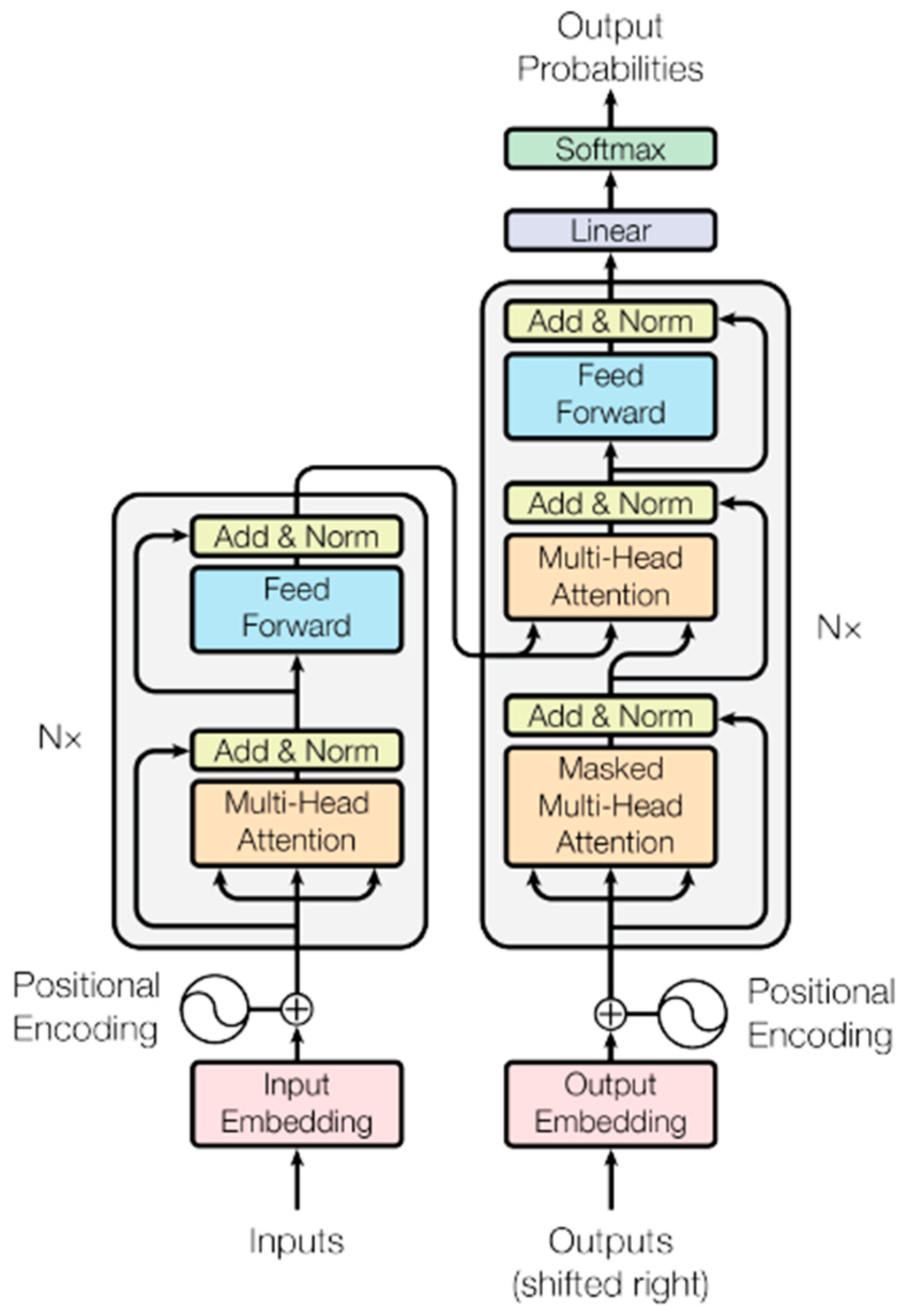
Figure 1.
Block diagram of the Transformer model from the paper “Attention is all you need” [
1].
Figure 1.
Block diagram of the Transformer model from the paper “Attention is all you need” [
1].
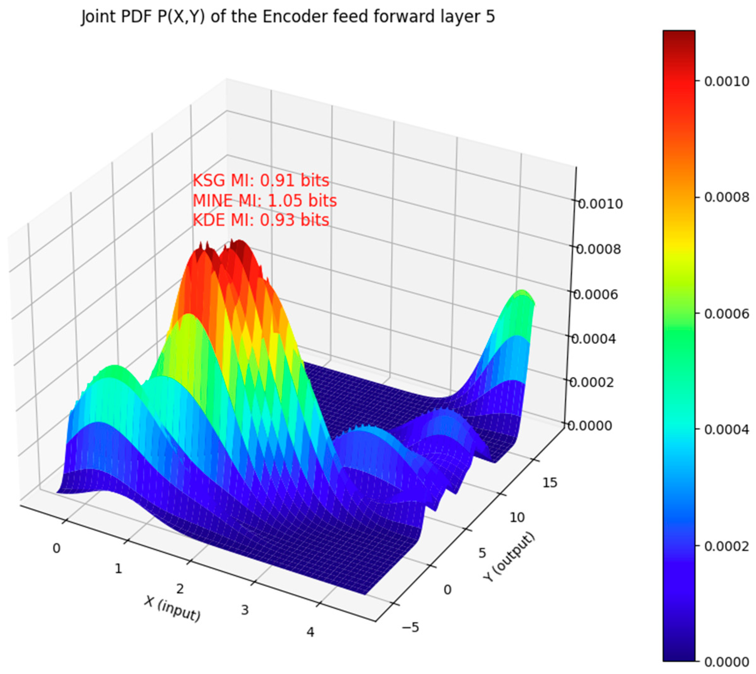
Figure 2.
Comparison of the MI estimate with the KSG, MINE, and KDE methods for the input and output vectors that are jointly distributed as shown. The input and output vectors are from the feedforward neural network of the layer 5 encoder sub-layer of the Transformer model. In this case, the mutual information computed by all three estimators is within ±0.14 bits of each other.
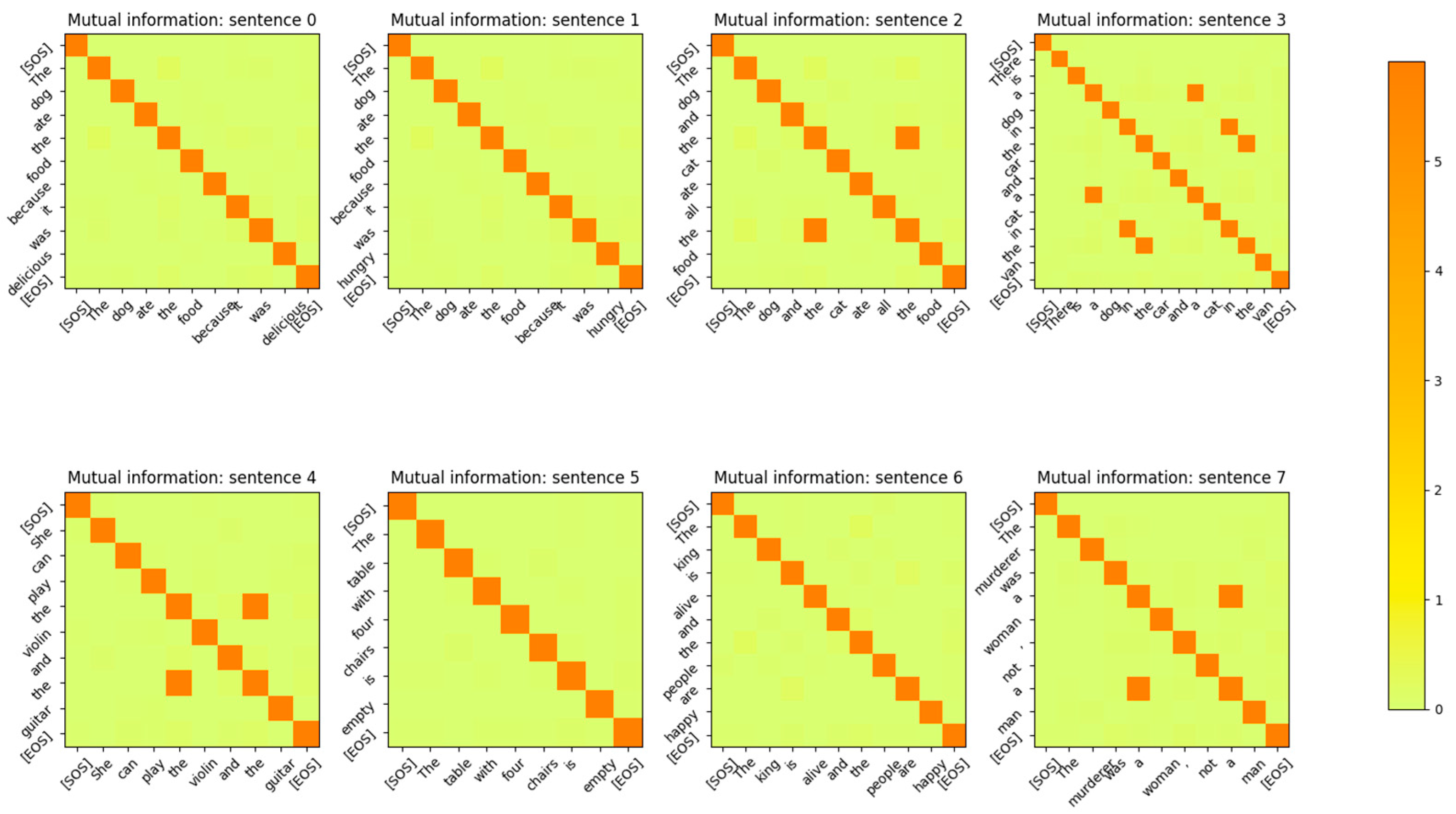
Figure 3.
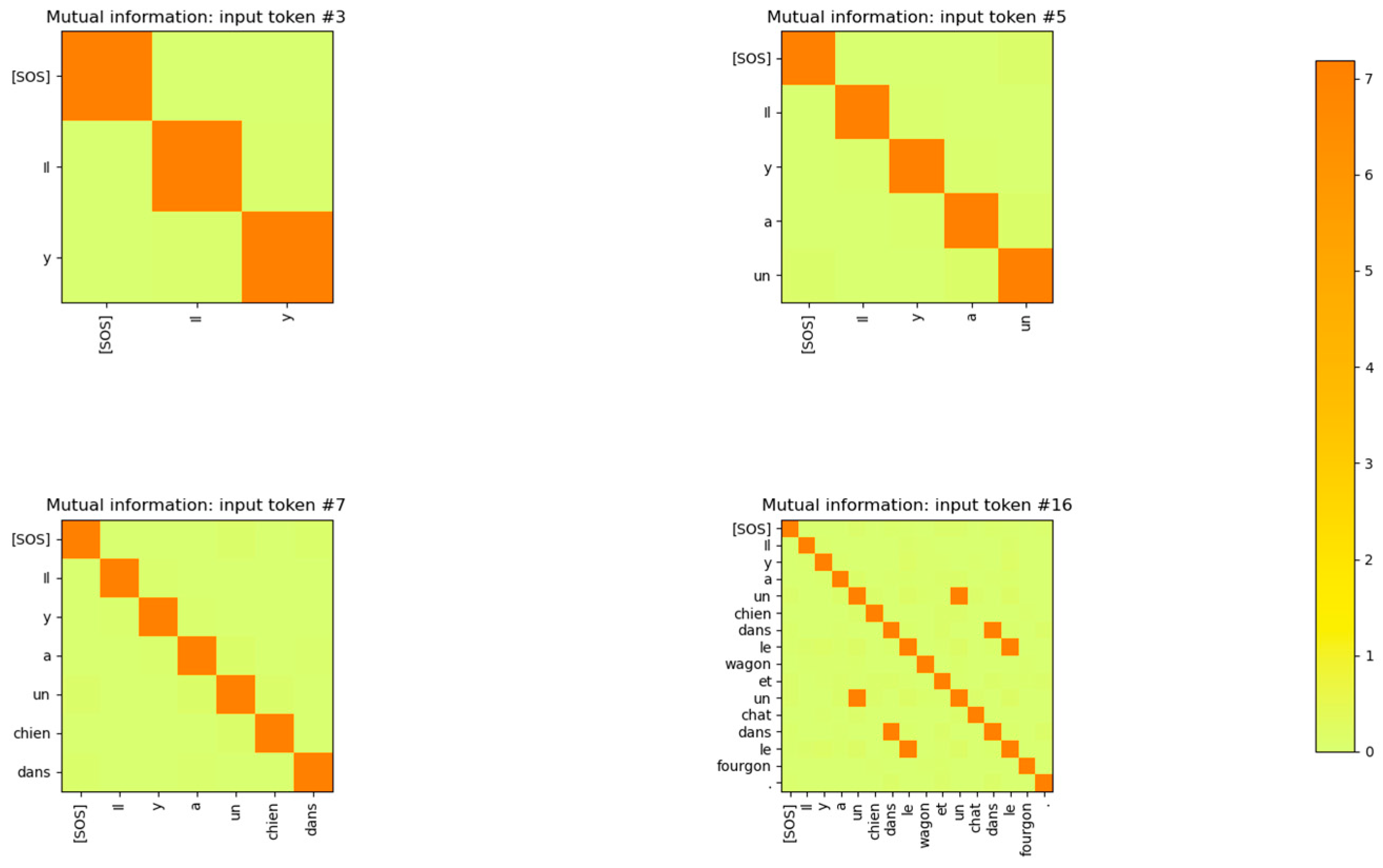
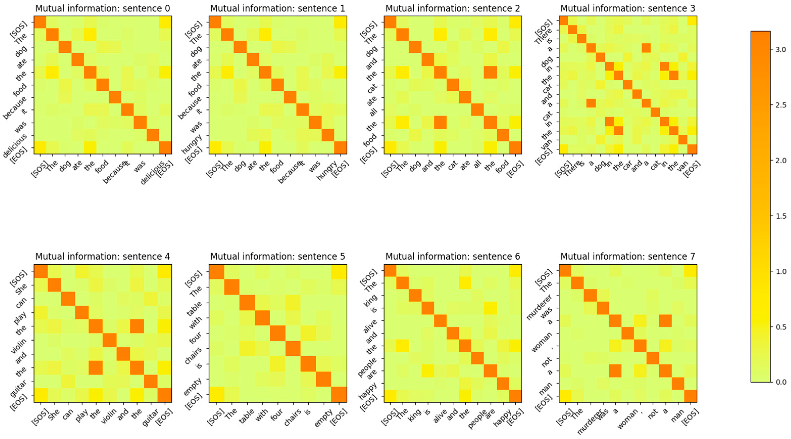
Mutual Information between the Input Embedding output vectors for at the end of the last epoch of training. The input sentences are from the validation set. The same tokens, irrespective of the position in the sentence, have high MI. Embedding vectors for different tokens are mutually independent. The diagonal represents the entropy of the token. Some token vectors that correspond to the same word but at a different position in the sentence have a high MI with the token at a different position. This shows that no positional information is encoded in the word embedding layer.
Figure 3.
Mutual Information between the Input Embedding output vectors for at the end of the last epoch of training. The input sentences are from the validation set. The same tokens, irrespective of the position in the sentence, have high MI. Embedding vectors for different tokens are mutually independent. The diagonal represents the entropy of the token. Some token vectors that correspond to the same word but at a different position in the sentence have a high MI with the token at a different position. This shows that no positional information is encoded in the word embedding layer.
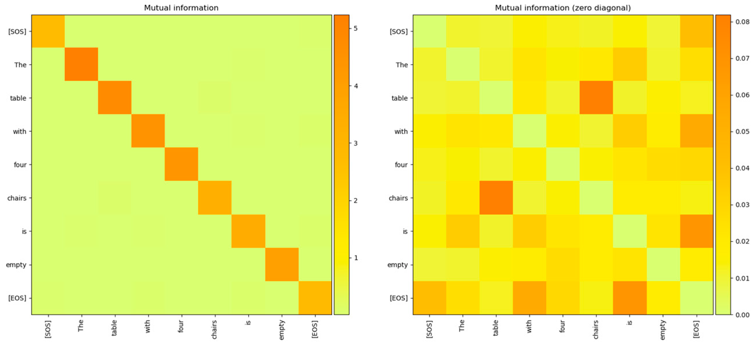
Figure 4.
The mutual information between the word embedding vectors plotted with and without the diagonal zeroed out to expose the low values of the Mutual Information between different token vectors. The picture on the right is with the diagonals zeroed out and it clearly shows that the mutual information of the token vector distribution with other vectors is very low, making the distributions independent of each other.
Figure 5.
MI between the rows of the decoder’s word embedding layer output matrix for each token input to this layer. The decoder’s output is concatenated with the previous output and fed as input to the word embedding layer. It is evident that the output vectors of different tokens are mutually independent from each other.
Figure 6.
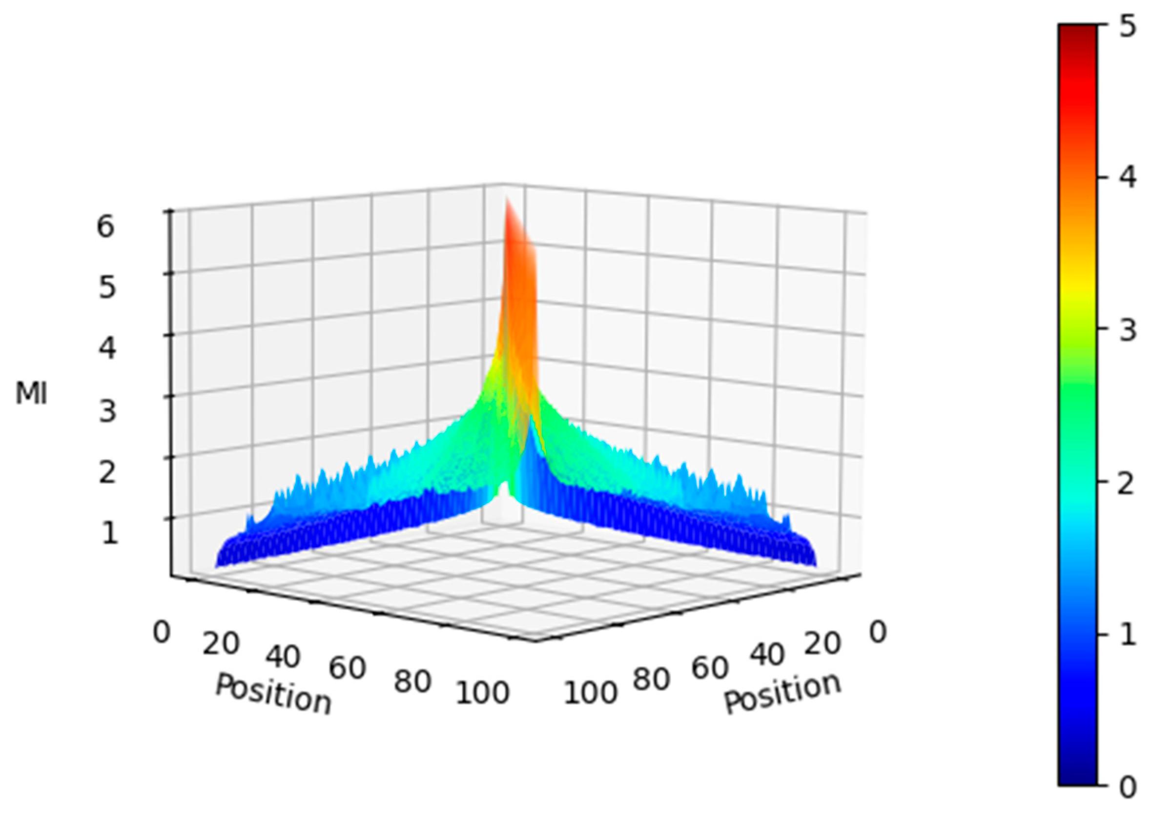
Mutual Information between the Positional Encoding vectors for seq length = 100 and (side view). The MI gradually tapers off with the position delta between tokens.
Figure 6.
Mutual Information between the Positional Encoding vectors for seq length = 100 and (side view). The MI gradually tapers off with the position delta between tokens.
Figure 7.
Mutual Information between the Positional Encoding vectors for seq length = 100, (top view). Tokens that are 20 positions away have an MI of about 3 bits.
Figure 7.
Mutual Information between the Positional Encoding vectors for seq length = 100, (top view). Tokens that are 20 positions away have an MI of about 3 bits.
Figure 8.
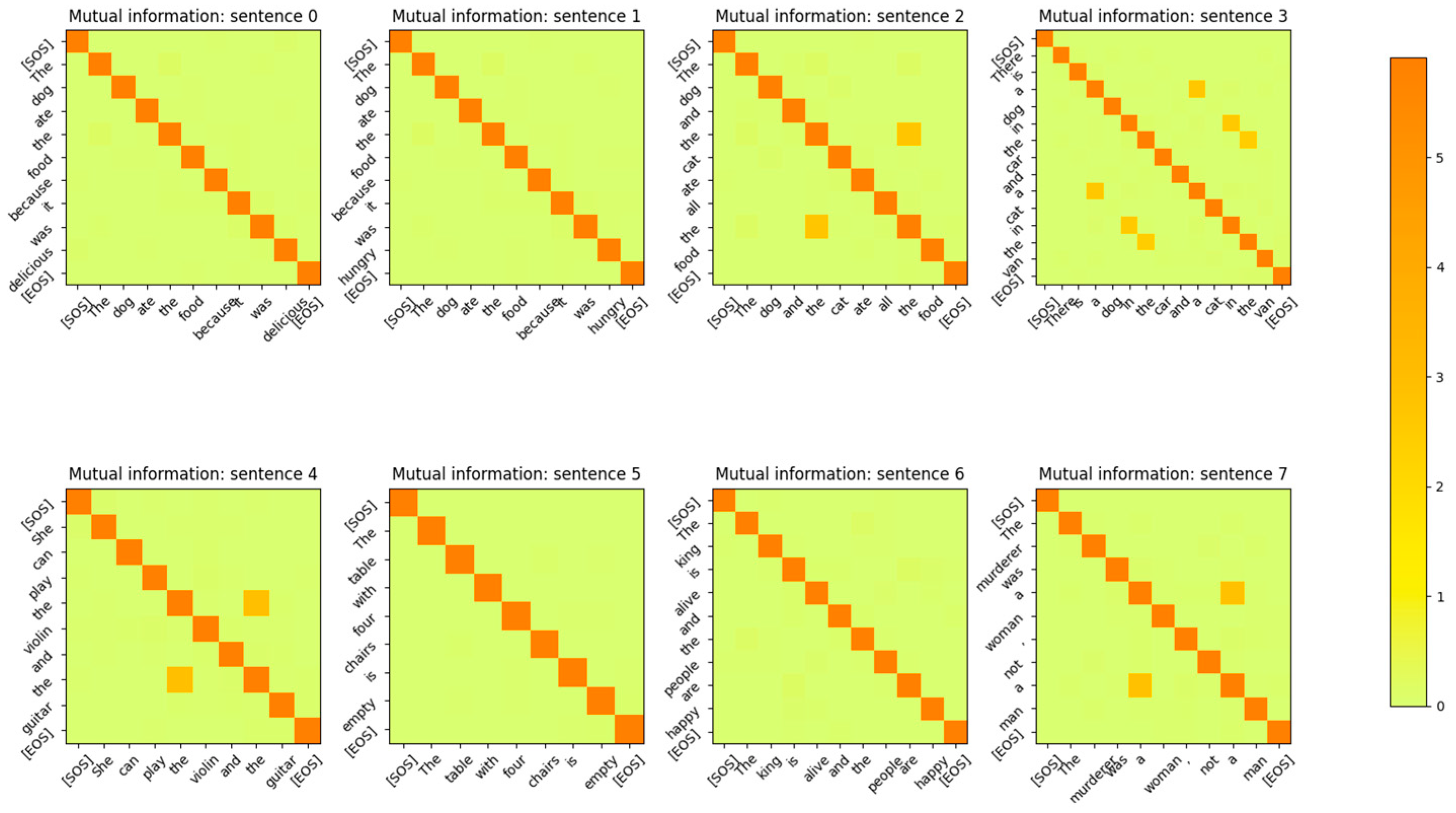
Mutual Information between the vectors of the Positional Encoding layer output for the sentences in the validation dataset. Comparing these plots to
Figure 3 shows that the MI of the same tokens at different positions has reduced from 5 bits to 2 bits due to the addition of positional information.
Figure 8.
Mutual Information between the vectors of the Positional Encoding layer output for the sentences in the validation dataset. Comparing these plots to
Figure 3 shows that the MI of the same tokens at different positions has reduced from 5 bits to 2 bits due to the addition of positional information.
Figure 9.
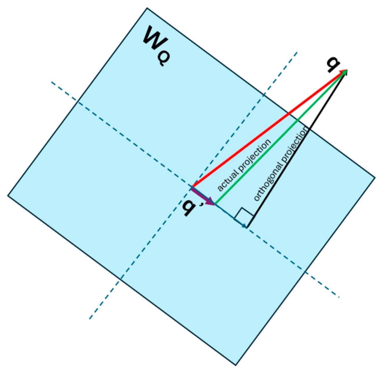
Projection of the input vector q to the column space of is not orthogonal.
Figure 9.
Projection of the input vector q to the column space of is not orthogonal.
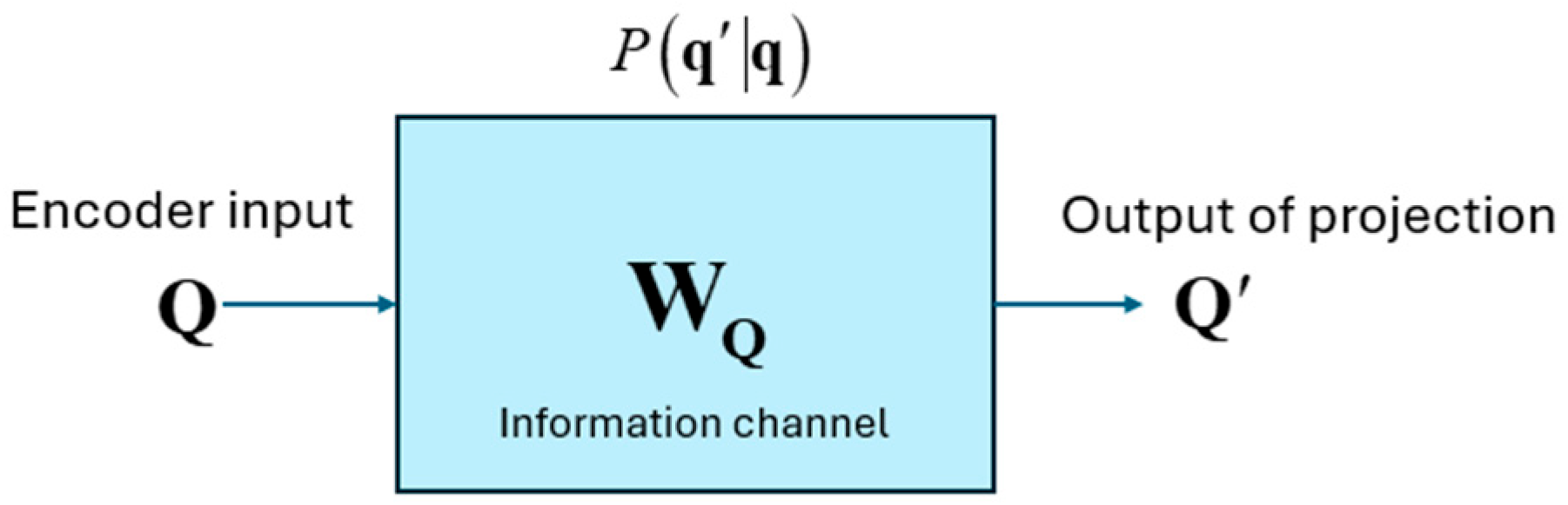
Figure 10.
Projection matrix as an information channel.
Figure 10.
Projection matrix as an information channel.
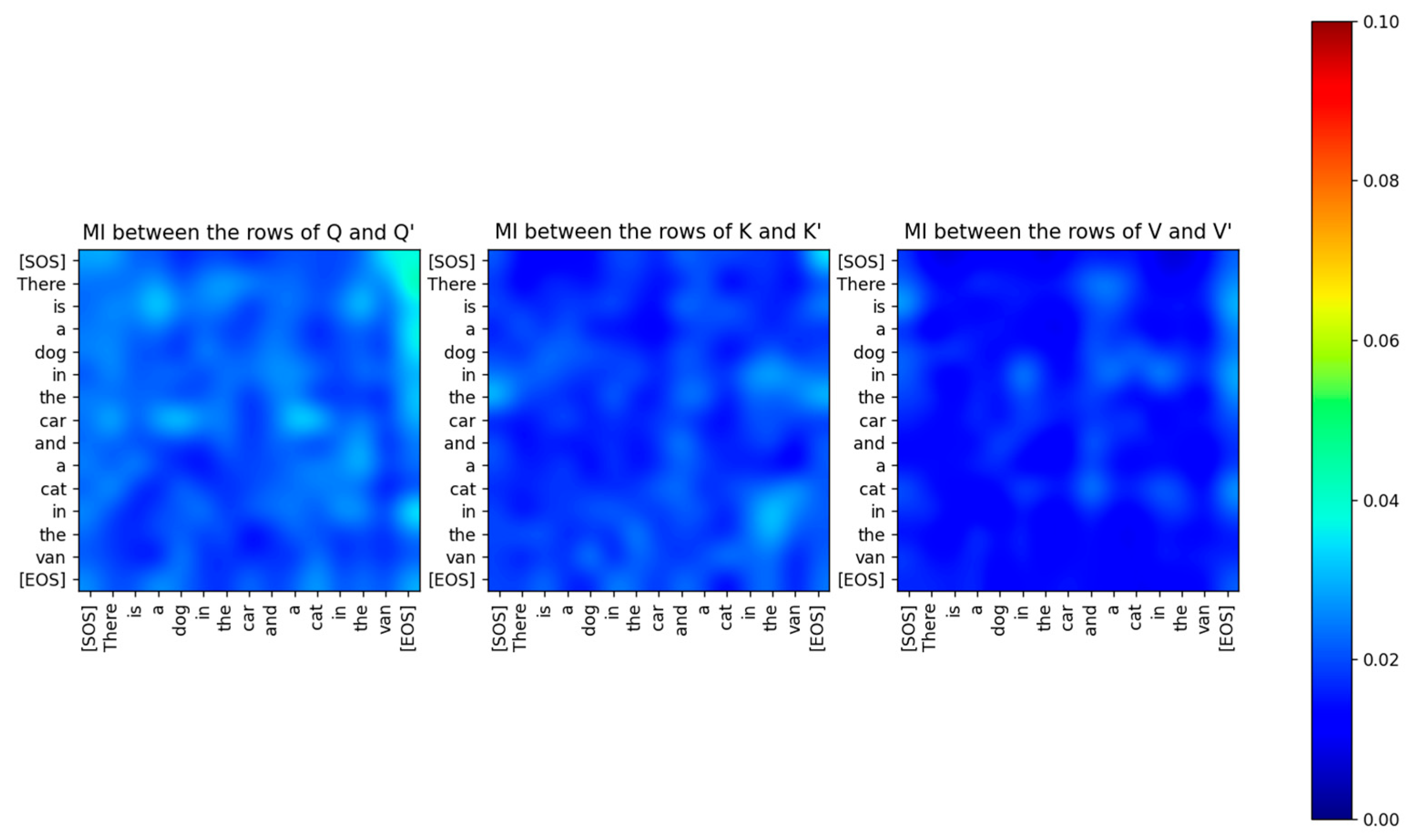
Figure 11.
The Mutual Information (MI) between the rows of and for attention layer 2 for a specific sentence. The MI is very low even between the same tokens which shows that the vectors and are mutually independent after the projection. All the attention layers show the same behavior.
Figure 11.
The Mutual Information (MI) between the rows of and for attention layer 2 for a specific sentence. The MI is very low even between the same tokens which shows that the vectors and are mutually independent after the projection. All the attention layers show the same behavior.
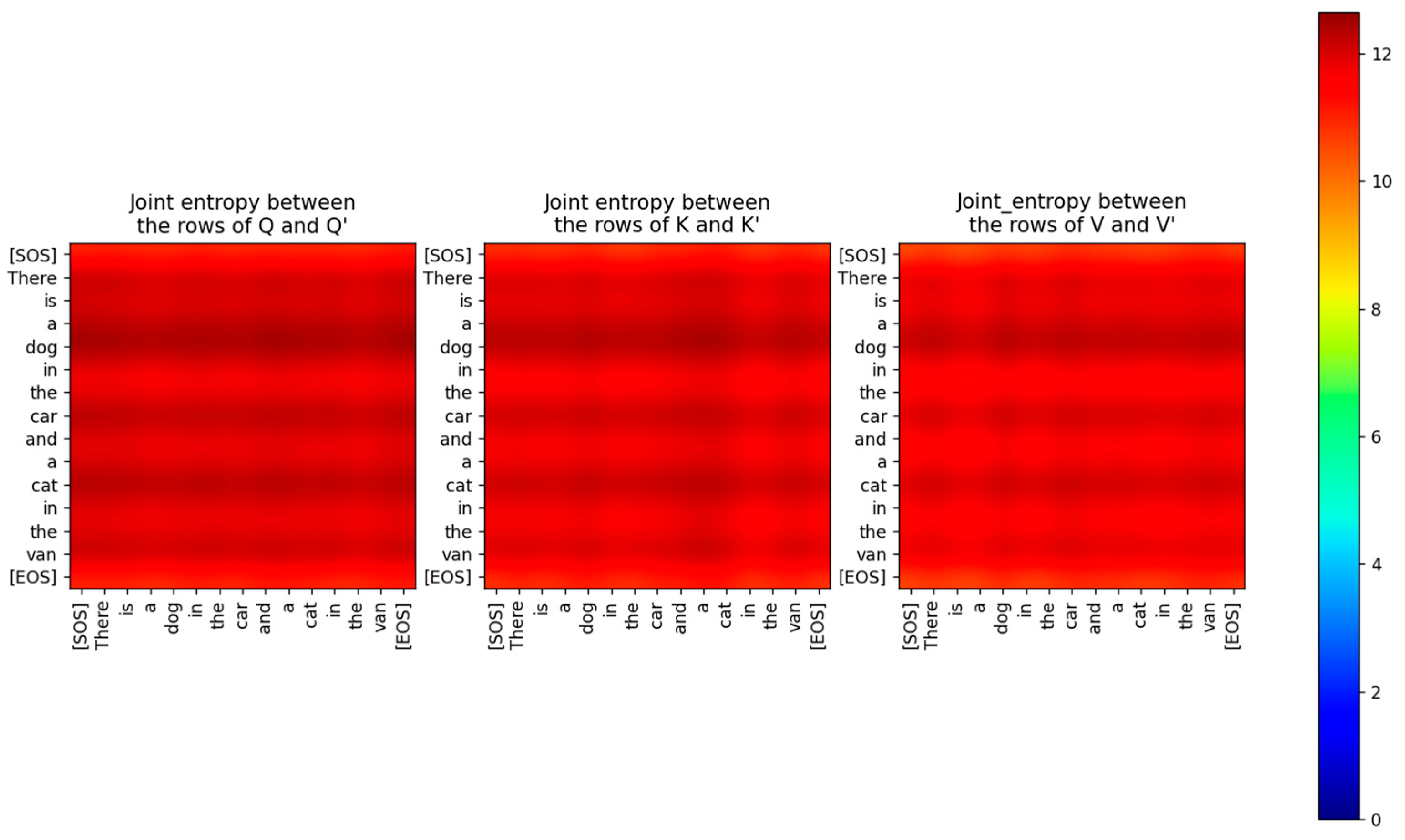
Figure 12.
Joint Entropy between Q, K, V and Q’, K’, V’ respectively.
Figure 12.
Joint Entropy between Q, K, V and Q’, K’, V’ respectively.
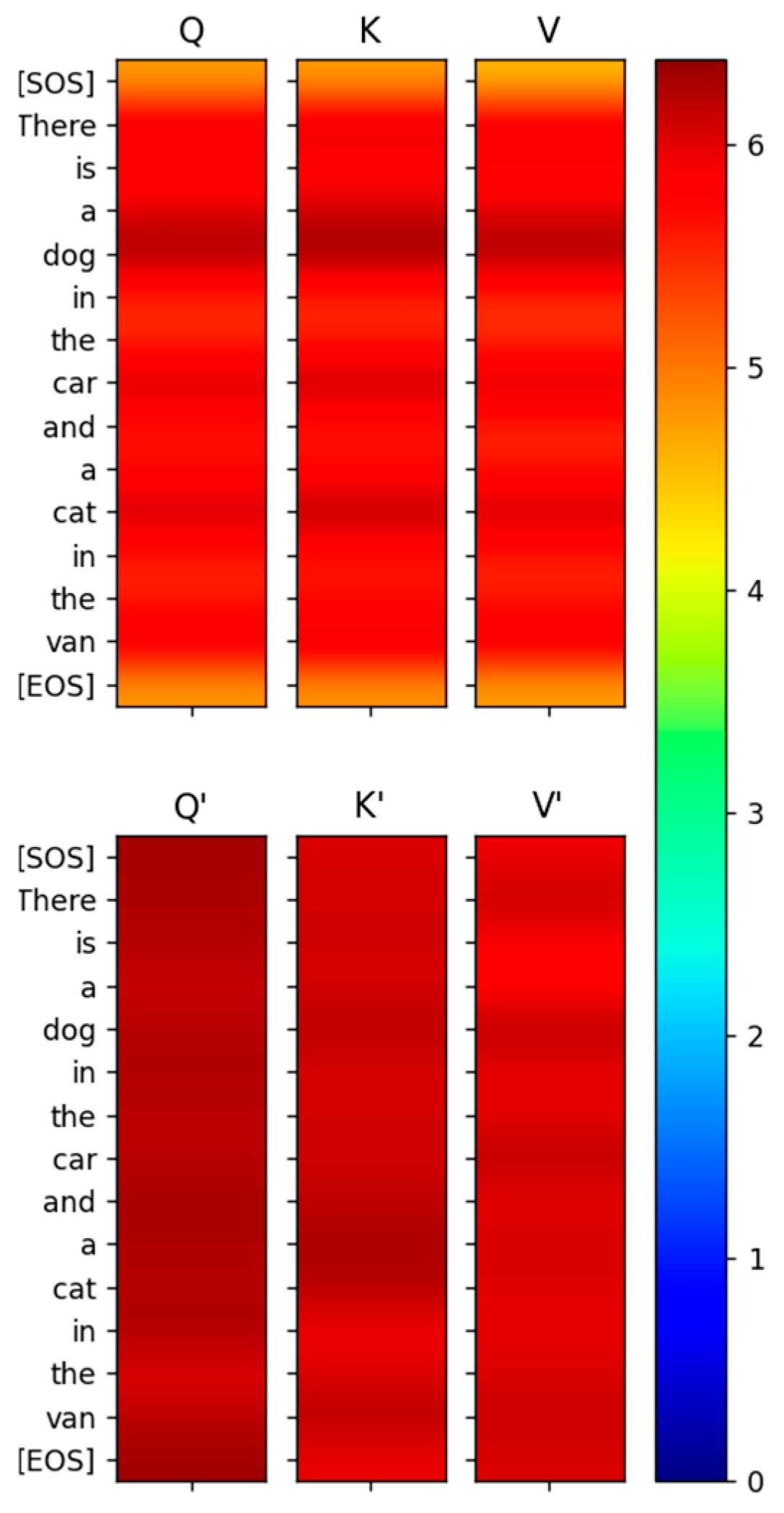
Figure 13.
Entropy of the rows of Q, K, V and Q’, K’, V’ is high indicating high information content.
Figure 13.
Entropy of the rows of Q, K, V and Q’, K’, V’ is high indicating high information content.
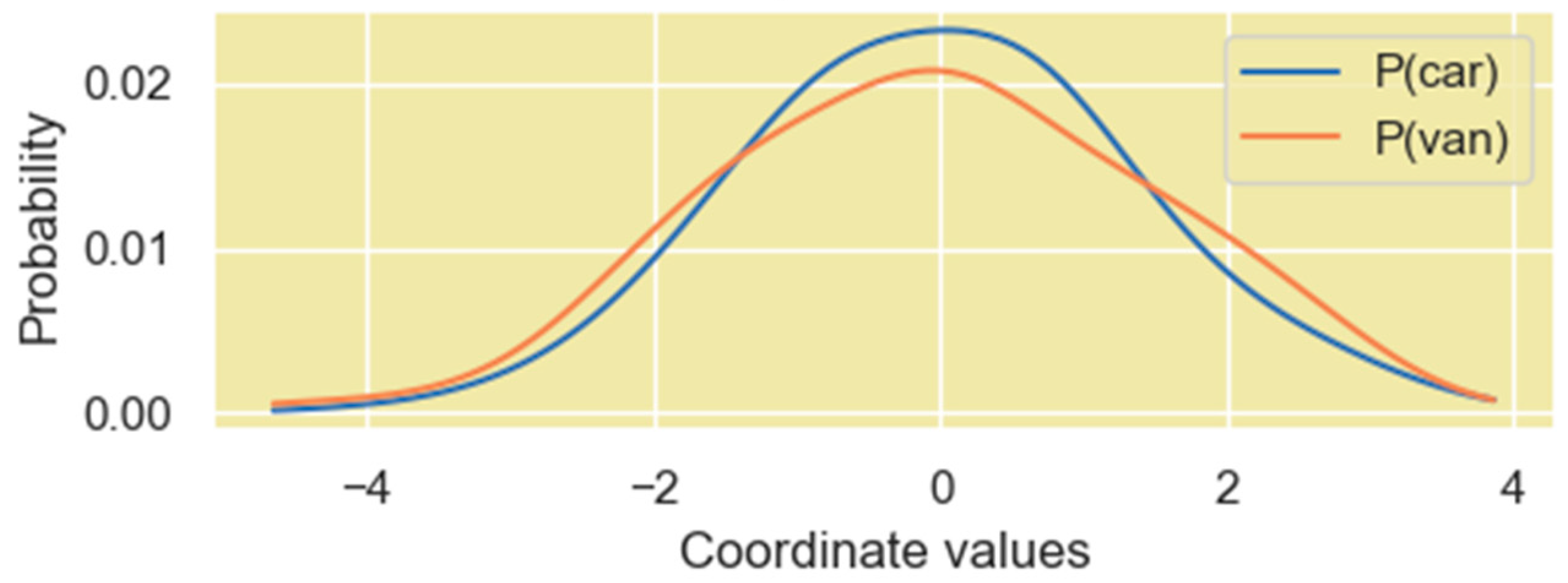
Figure 14.
PDF of the vector coordinate values when the coordinates are viewed as numerical outcomes of a single random variable. The vectors in the plot correspond to the words “car” and “van” in the Q’ matrix.
Figure 14.
PDF of the vector coordinate values when the coordinates are viewed as numerical outcomes of a single random variable. The vectors in the plot correspond to the words “car” and “van” in the Q’ matrix.
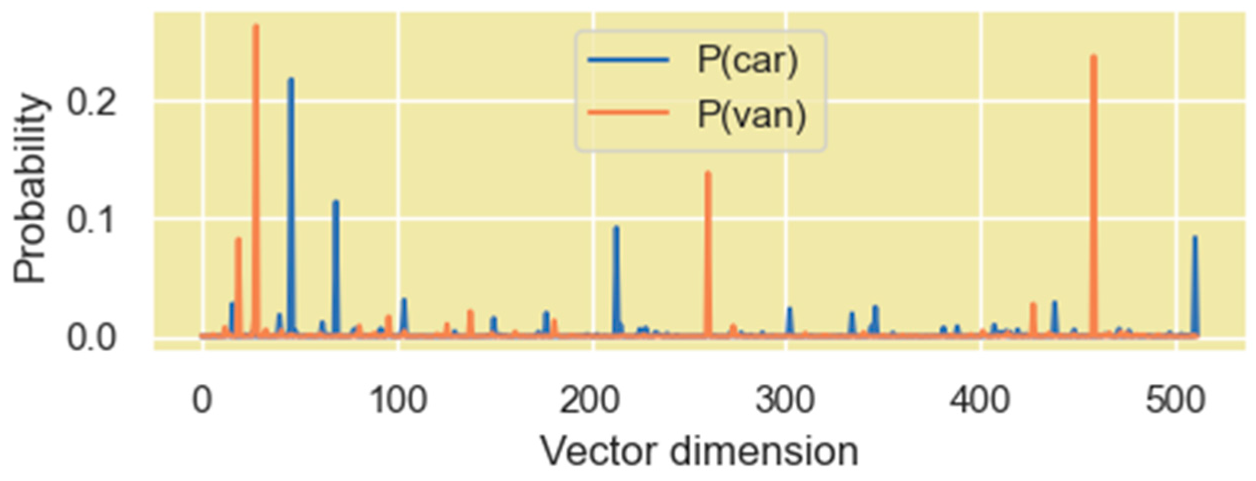
Figure 15.
PDF of the vector coordinate values when the coordinates are viewed as energy levels of the individual microstates. The vectors correspond to the word “car” and “van” in the Q’ matrix.
Figure 15.
PDF of the vector coordinate values when the coordinates are viewed as energy levels of the individual microstates. The vectors correspond to the word “car” and “van” in the Q’ matrix.
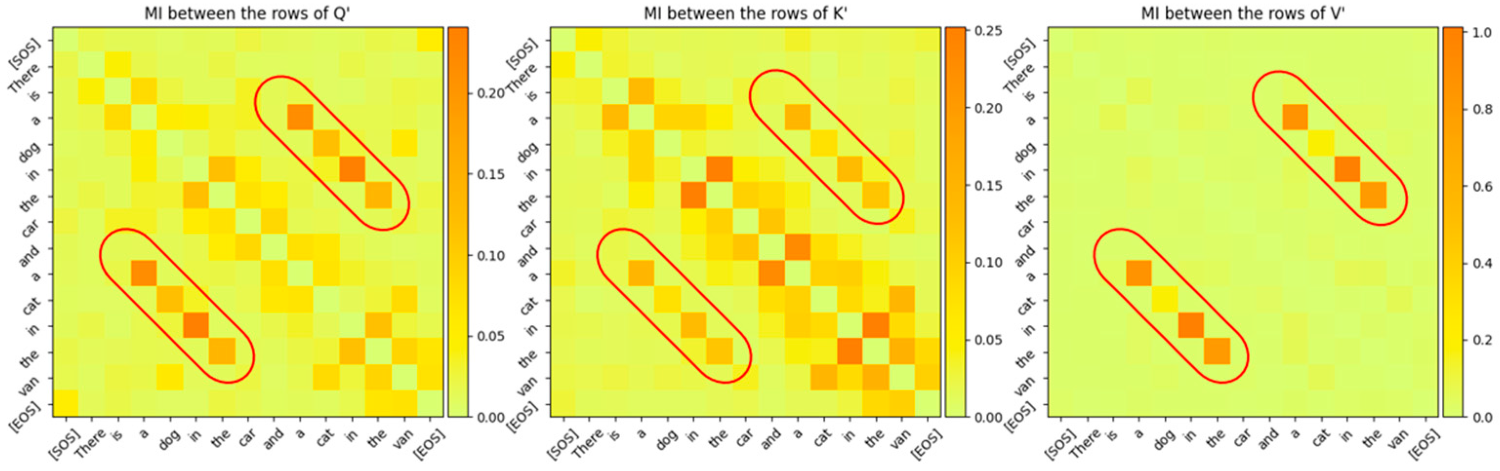
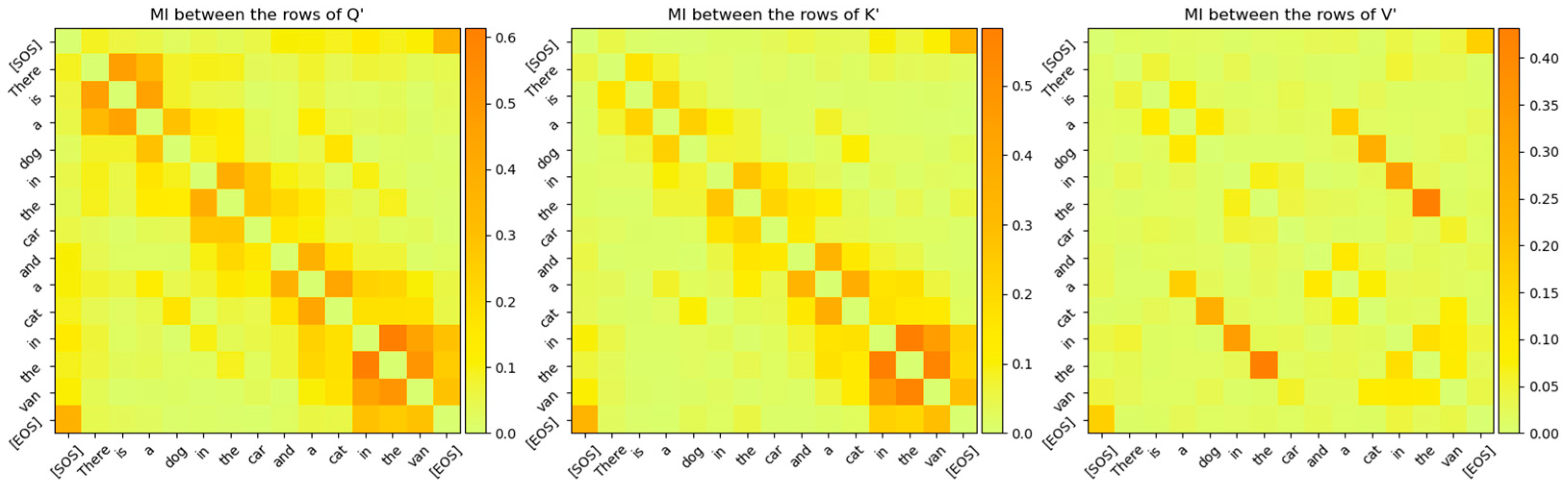
Figure 16.
Mutual Information between the rows of Q’, K’, V’ for Attention Layer 0. The relationship between the word sequence “cat in the van” and “dog in the car” is clearly visible even though these vectors are projected to high-dimensional vector space. The diagonal entries, which are entropies of the token vectors, have been intentionally zeroed out so that the other MI values are visible.
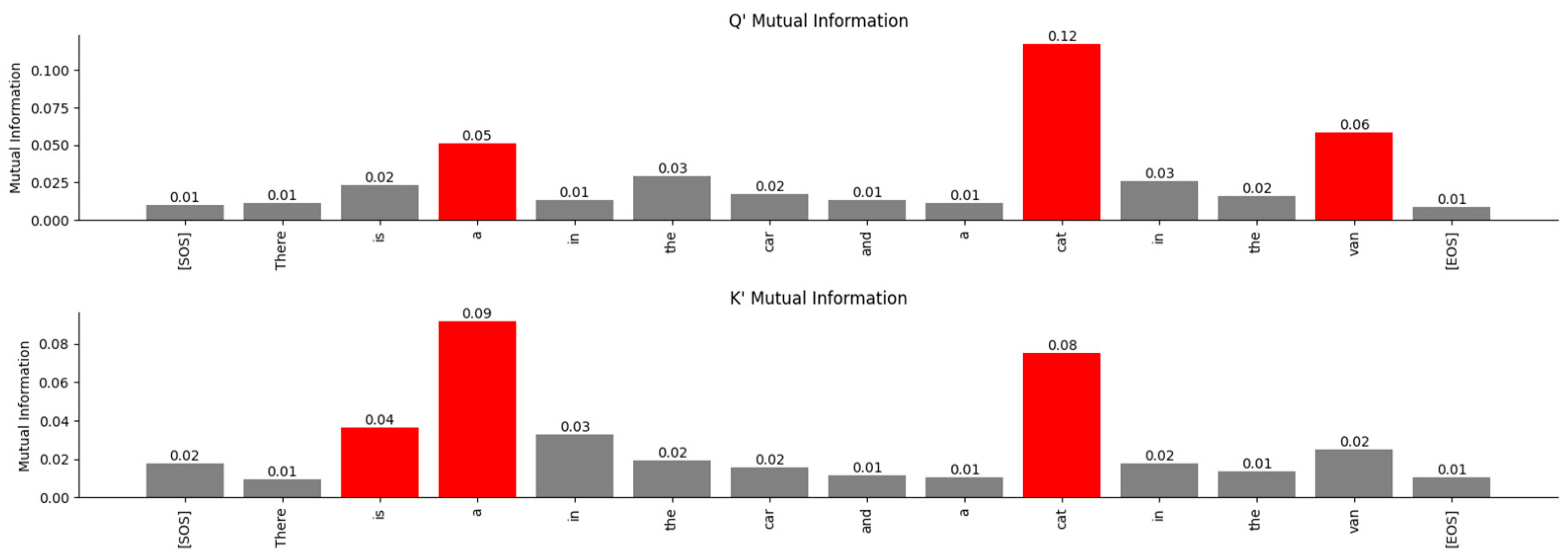
Figure 17.
Attention layer 0 relationships between the word “dog” and the other words in the Q’ and K’ matrices in high-dimensional space exposed by MI. The Transformer associates the word “dog” with the words “a”, “cat”, “van” in the Q’ matrix and the words “is”, “a”, “cat” in the K’ matrix.
Figure 17.
Attention layer 0 relationships between the word “dog” and the other words in the Q’ and K’ matrices in high-dimensional space exposed by MI. The Transformer associates the word “dog” with the words “a”, “cat”, “van” in the Q’ matrix and the words “is”, “a”, “cat” in the K’ matrix.
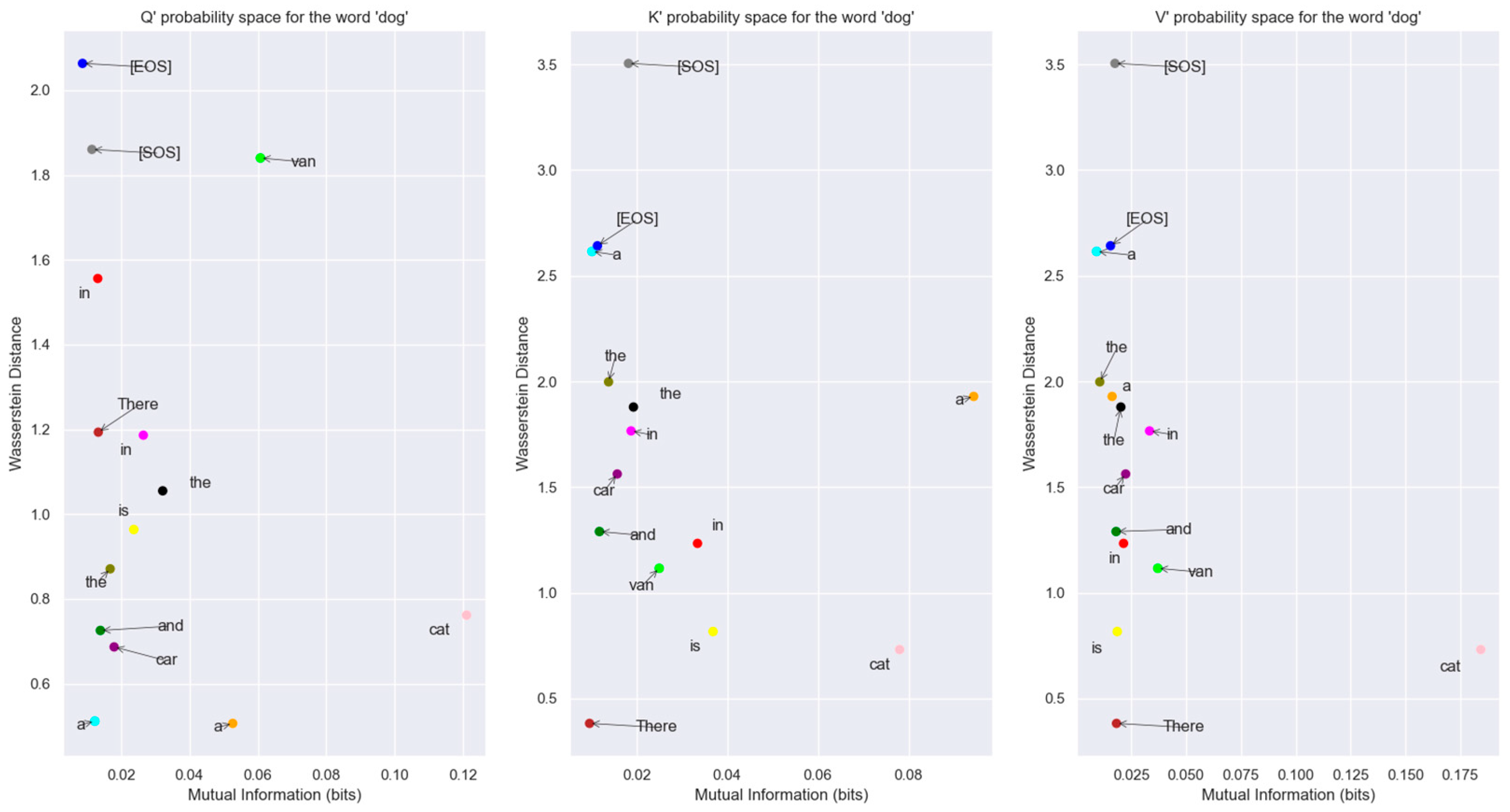
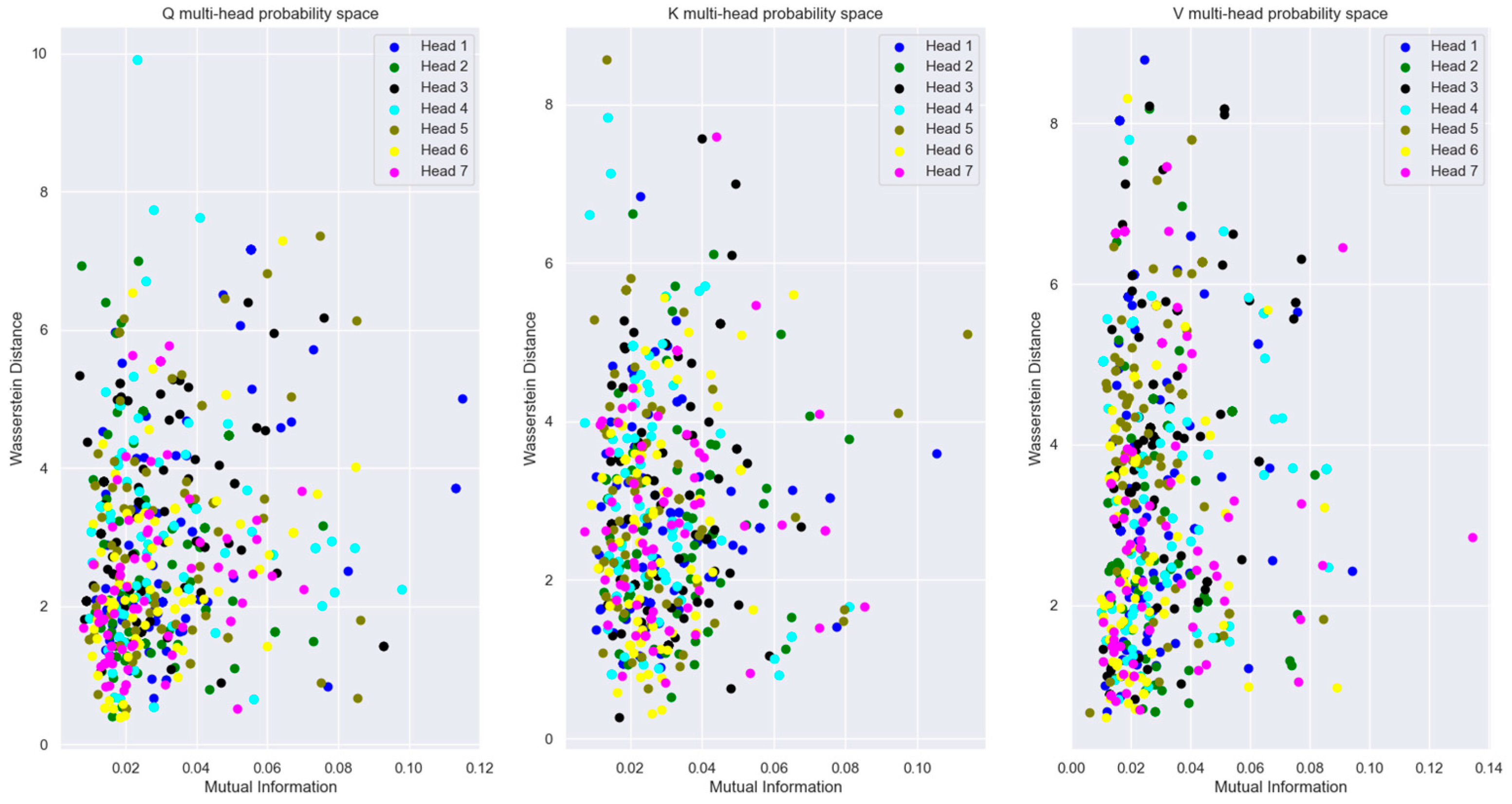
Figure 18.
Word vectors for Q’, K’, V’ prime in The Mutual Information vs. Wasserstein distance plane. Each of the words in this plane is compared to the word vector for “dog”. Points that are closer to the bottom right part of each plot have their distributions closer to the word dog. The word “cat” is closest to the word “dog” in probability space. This view allows us to understand the relationship between words in probability space.
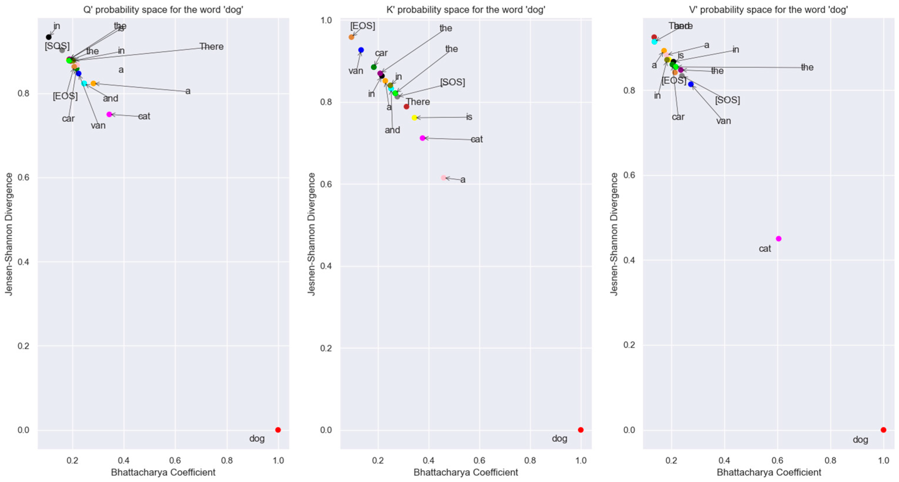
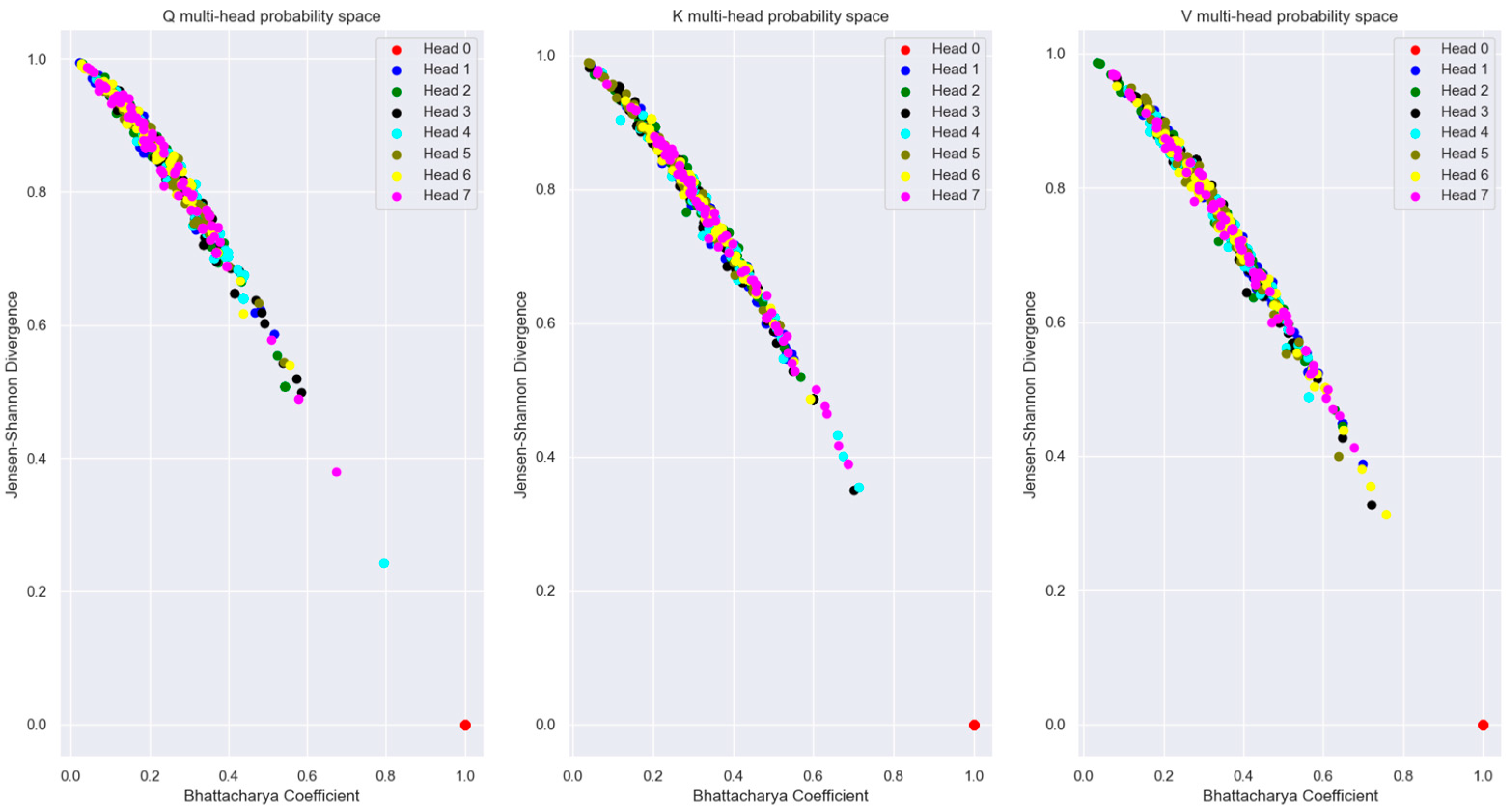
Figure 19.
Plot of the different word tokens vectors of Q’, K’, V’ in probability space. The points that are closer to the lower right-hand corner in each graph are closer in probability space to the word vector “dog”. From this plot, it is obvious that the Boltzmann distributions of the individual vectors don’t overlap with the vector distribution for “dog”. Also, the distributions are divergent from each other. The vector distribution for “cat” is the closest to the vector distribution for “dog” in this plane.
Figure 20.
Mutual Information between the rows of for Attention Layer 3. The relationships between the word sequences “There is a”, “in the car”, and “in the van” are clearly visible even though these vectors are projected to a high-dimensional vector space. The darker colored MIs are different compared to attention layer 0, indicating that this layer is focused on different relationships between words compared to attention layer 0. The diagonal entries, which are entropies of the token vectors, have been intentionally zeroed out so that the other MI values are visible.
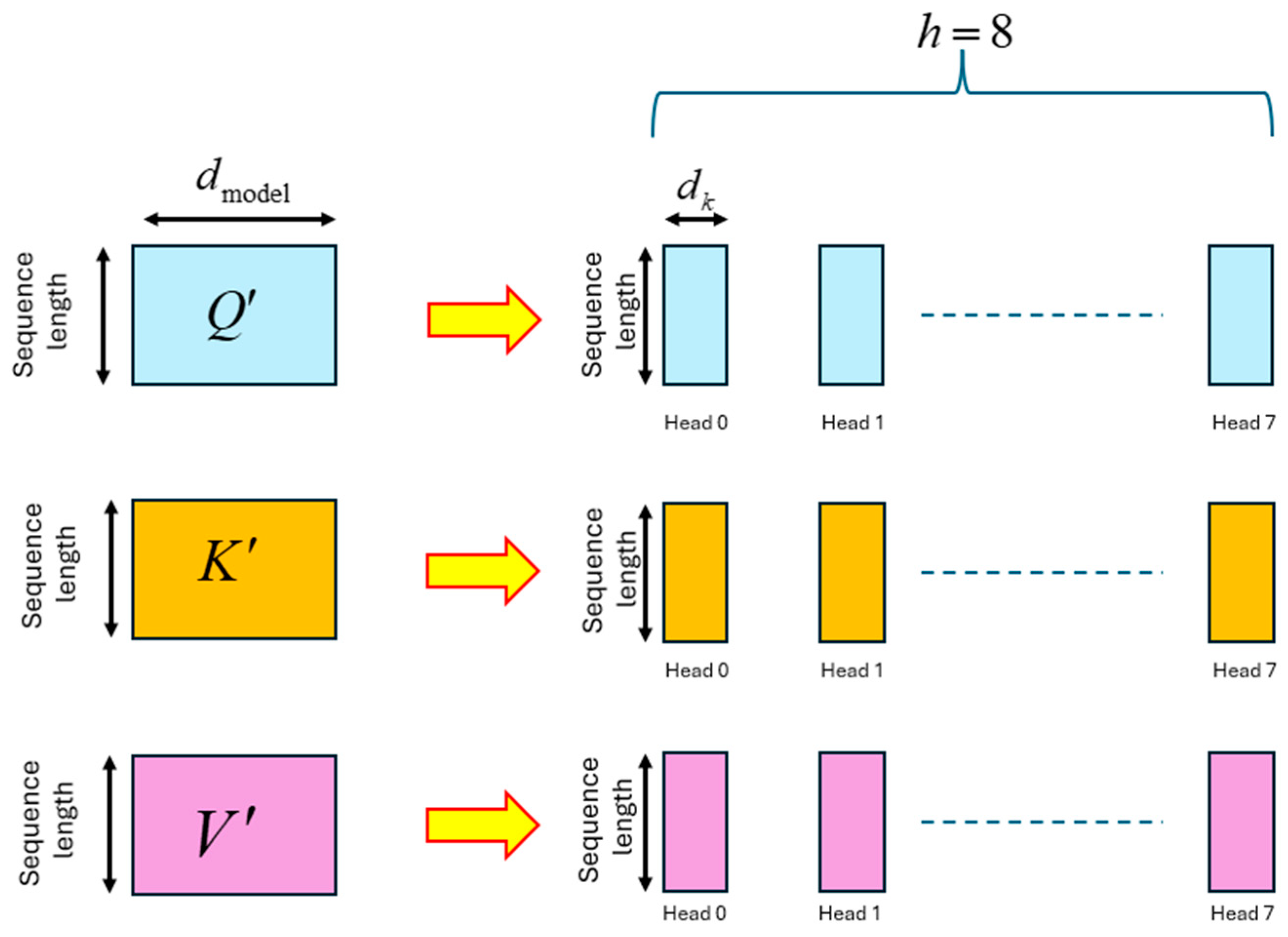
Figure 21.
Partitioning of the Q’, K’, V’ matrices into h = 8 sub-matrices for multi-head processing.
Figure 21.
Partitioning of the Q’, K’, V’ matrices into h = 8 sub-matrices for multi-head processing.
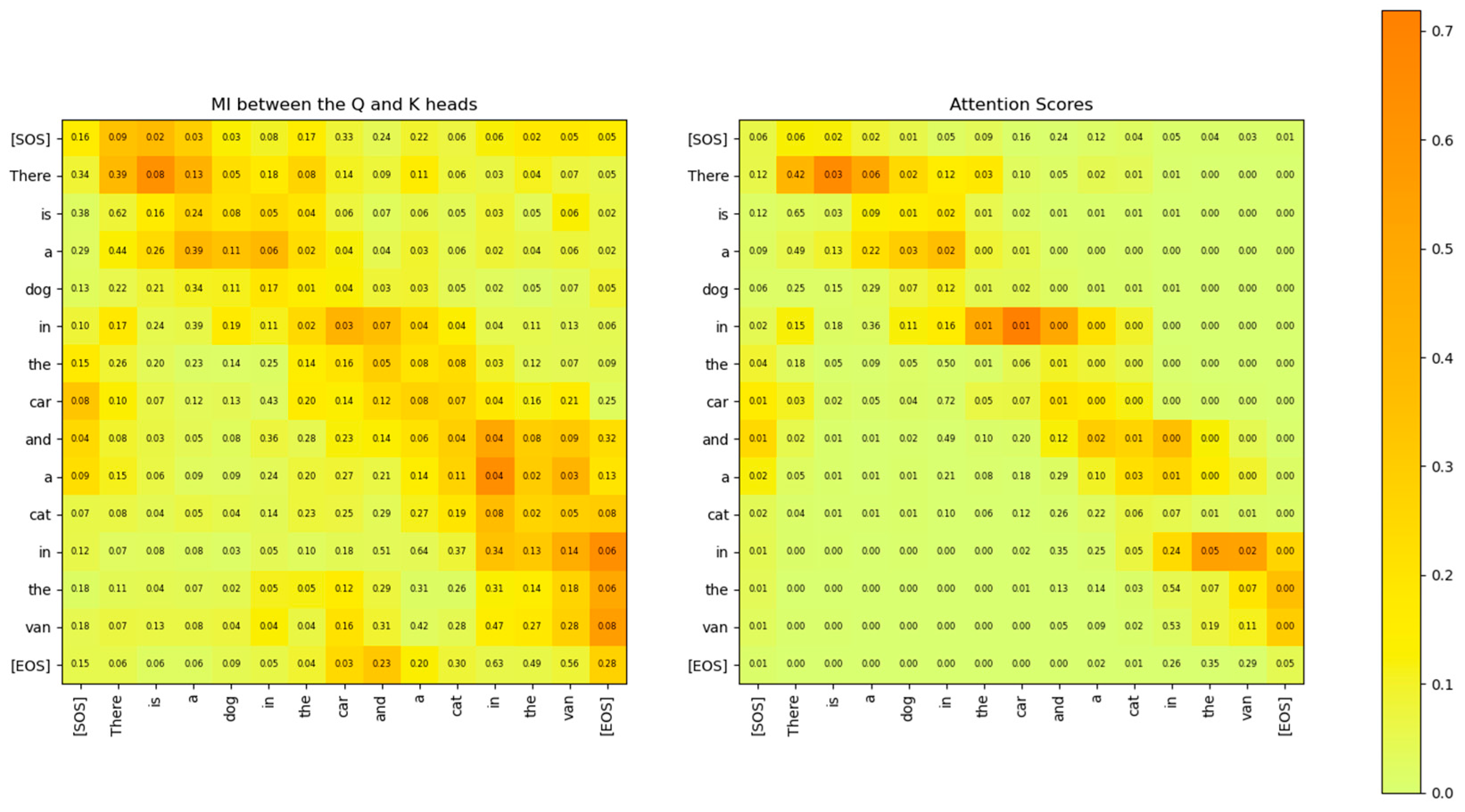
Figure 22.
Comparison of the Mutual Information between the Q and K heads (left) and the attention scores (right) for attention layer 2, head 2. The two matrices show similar relationships between the words of the sentence. However, the MI matrix exposes weaker relationships that are not visible in the attention scores matrix.
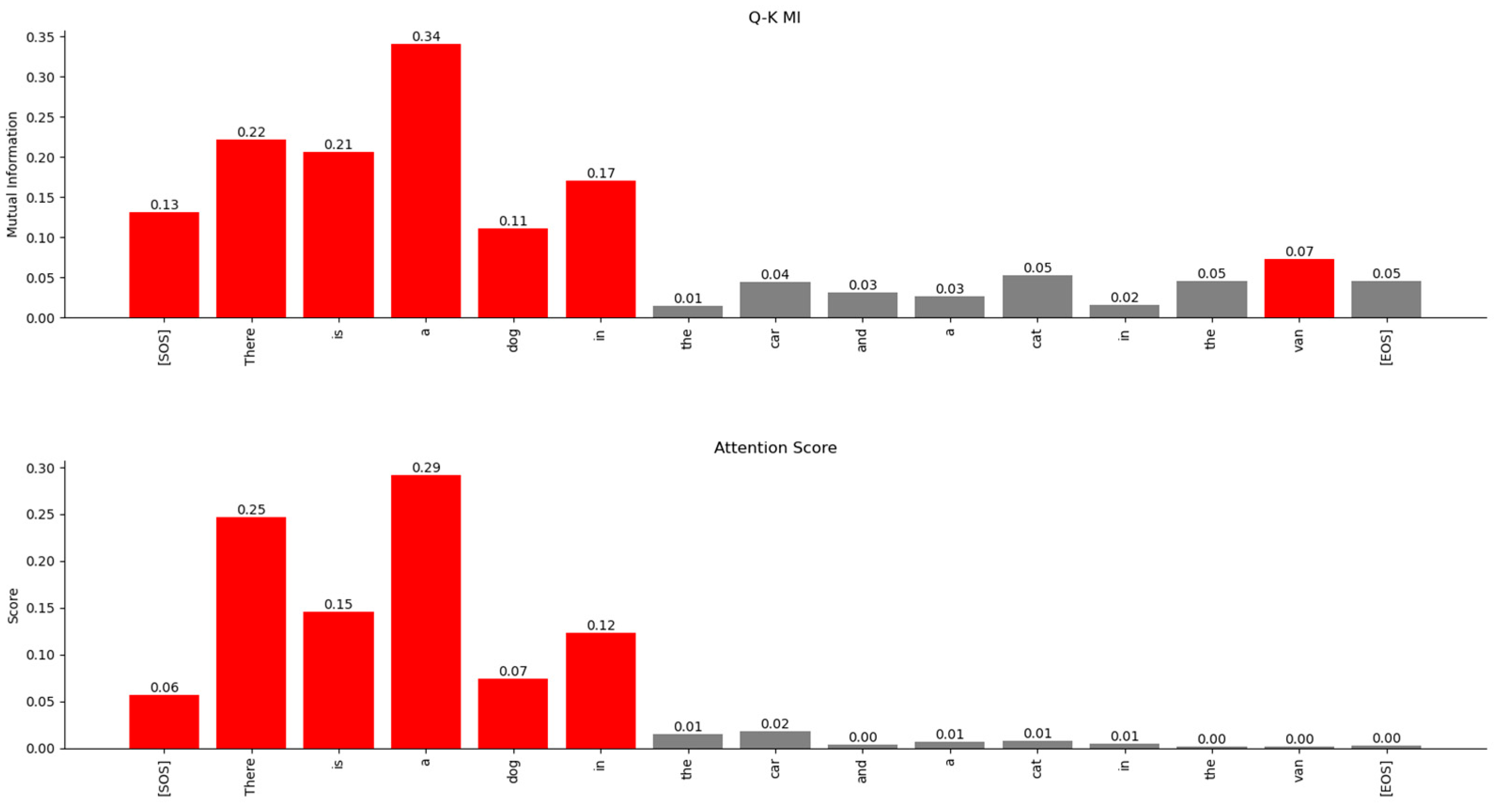
Figure 23.
Relationship of the word ‘dog’ with other words in the sentence. The MI-based relationships (top) and the Attention Scores-based relationships (bottom) show similar trends. However, MI exposes a weaker relationship with the word “van”, which is not visible in the Attention Scores matrix.
Figure 23.
Relationship of the word ‘dog’ with other words in the sentence. The MI-based relationships (top) and the Attention Scores-based relationships (bottom) show similar trends. However, MI exposes a weaker relationship with the word “van”, which is not visible in the Attention Scores matrix.
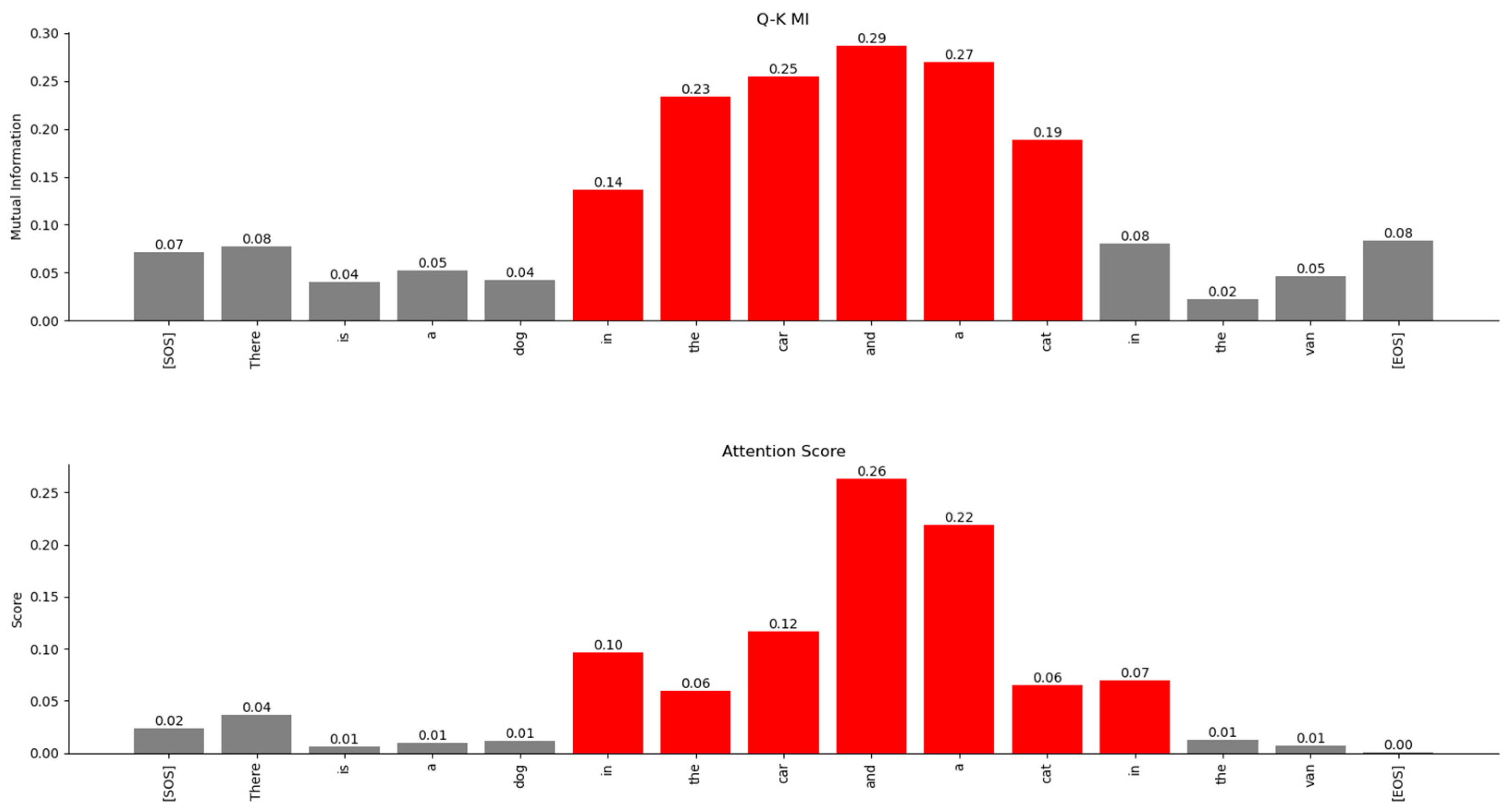
Figure 24.
Relationship of the word ‘car’ with other words in the sentence. The MI-based relationships (top) and the Attention Scores-based relationships (bottom) show similar trends. However, MI exposes a weaker relationship with the word “van,” which is not visible in the Attention Scores matrix.
Figure 24.
Relationship of the word ‘car’ with other words in the sentence. The MI-based relationships (top) and the Attention Scores-based relationships (bottom) show similar trends. However, MI exposes a weaker relationship with the word “van,” which is not visible in the Attention Scores matrix.
Figure 25.
Relationship of the word ‘cat’ with other words in the sentence. The MI-based relationships (top) and the Attention Scores-based relationships (bottom) show similar trends.
Figure 25.
Relationship of the word ‘cat’ with other words in the sentence. The MI-based relationships (top) and the Attention Scores-based relationships (bottom) show similar trends.
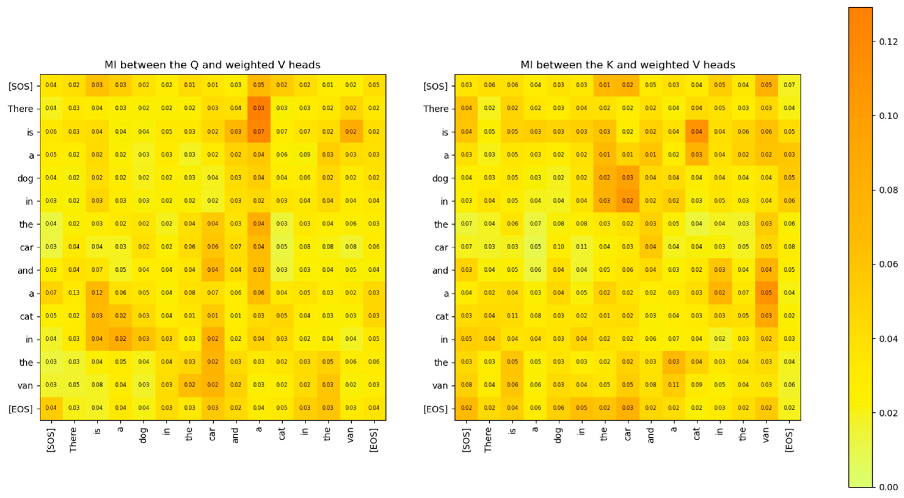
Figure 26.
MI between Q head and weighted V head, and the MI between the K head and weighted V head for attention layer 2 and head 2. The MI shows how much information from Q and K heads is contained in the weighted V head matrix.
Figure 26.
MI between Q head and weighted V head, and the MI between the K head and weighted V head for attention layer 2 and head 2. The MI shows how much information from Q and K heads is contained in the weighted V head matrix.
Figure 27.
Distribution of the same word vector coordinates in different attention layer heads with respect to head 0 of the encoder. The plots show that the Boltzmann distributions for the same words are sufficiently separated statistically between the different attention heads so that each head can attend to different latent parameters of the words. Several words from the validation dataset are plotted in this probability distribution plane.
Figure 28.
Plots of the same word vectors across multiple attention heads with reference to head 0. The plot shows that the coordinate distributions of the word vectors are not statistically far apart. However, the Mutual Information between the same word vectors across multiple attention heads is very low, making them mutually independent. Several words from the validation dataset are plotted in this figure.
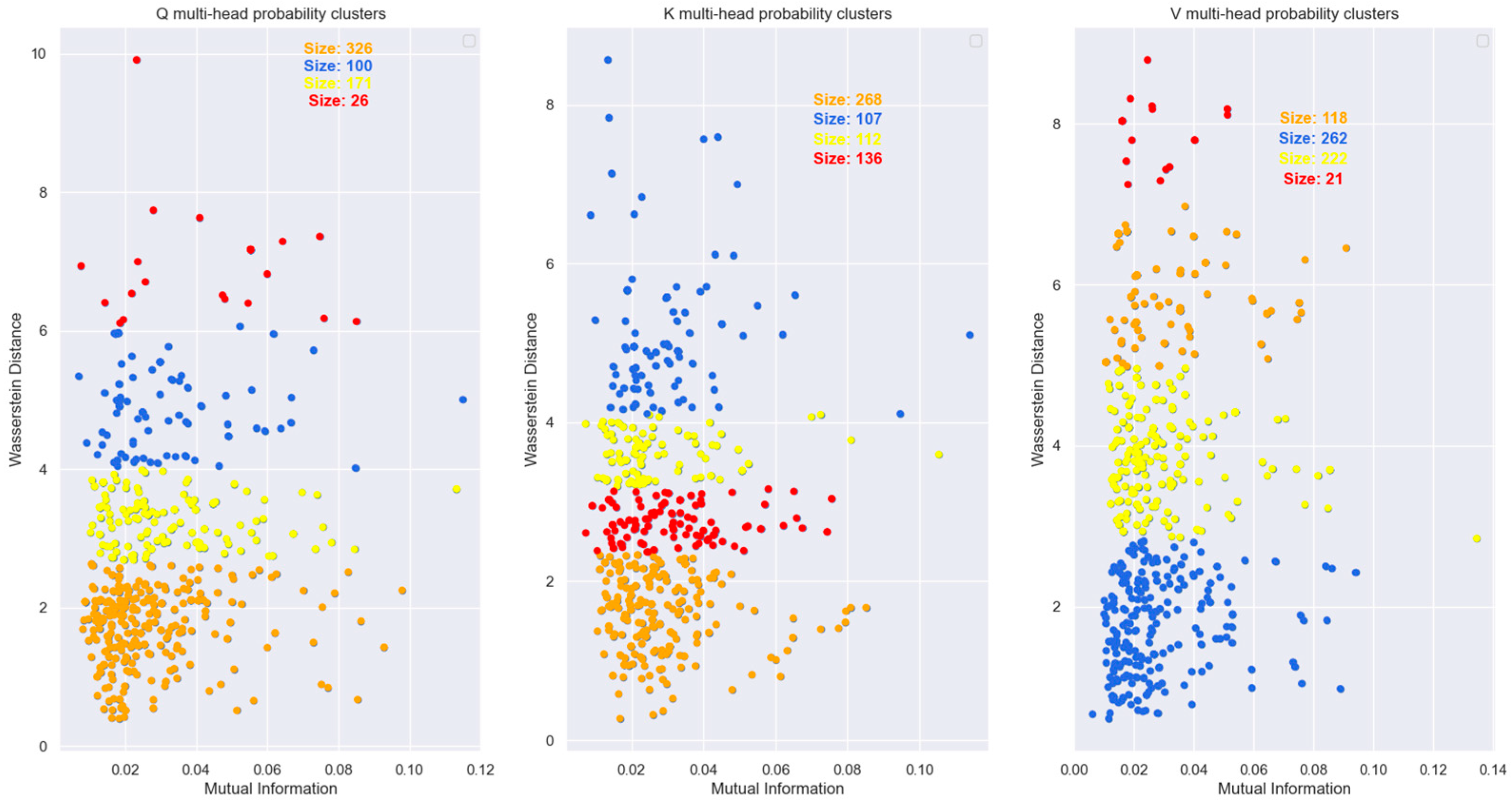
Figure 29.
Spectral clustering of the data points from
Figure 28. The clusters show that most of the points in the plane lie in a cluster with statistically similar coordinate distributions. However, the distribution of the same word vectors across the various heads are mutually independent.
Figure 29.
Spectral clustering of the data points from
Figure 28. The clusters show that most of the points in the plane lie in a cluster with statistically similar coordinate distributions. However, the distribution of the same word vectors across the various heads are mutually independent.
Figure 30.
Numerical verification of the supermodular property of mutual information for the encoder’s (left plot) and decoder’s (right plot) heads shows that the Transformer’s attention heads satisfy the inequality . This implies that the distributions of the heads are mutually independent. The supermodularity condition can be used as an upper bound for the number of attention heads. In other words, the number of attention heads cannot exceed a threshold that will violate the supermodularity constraint.
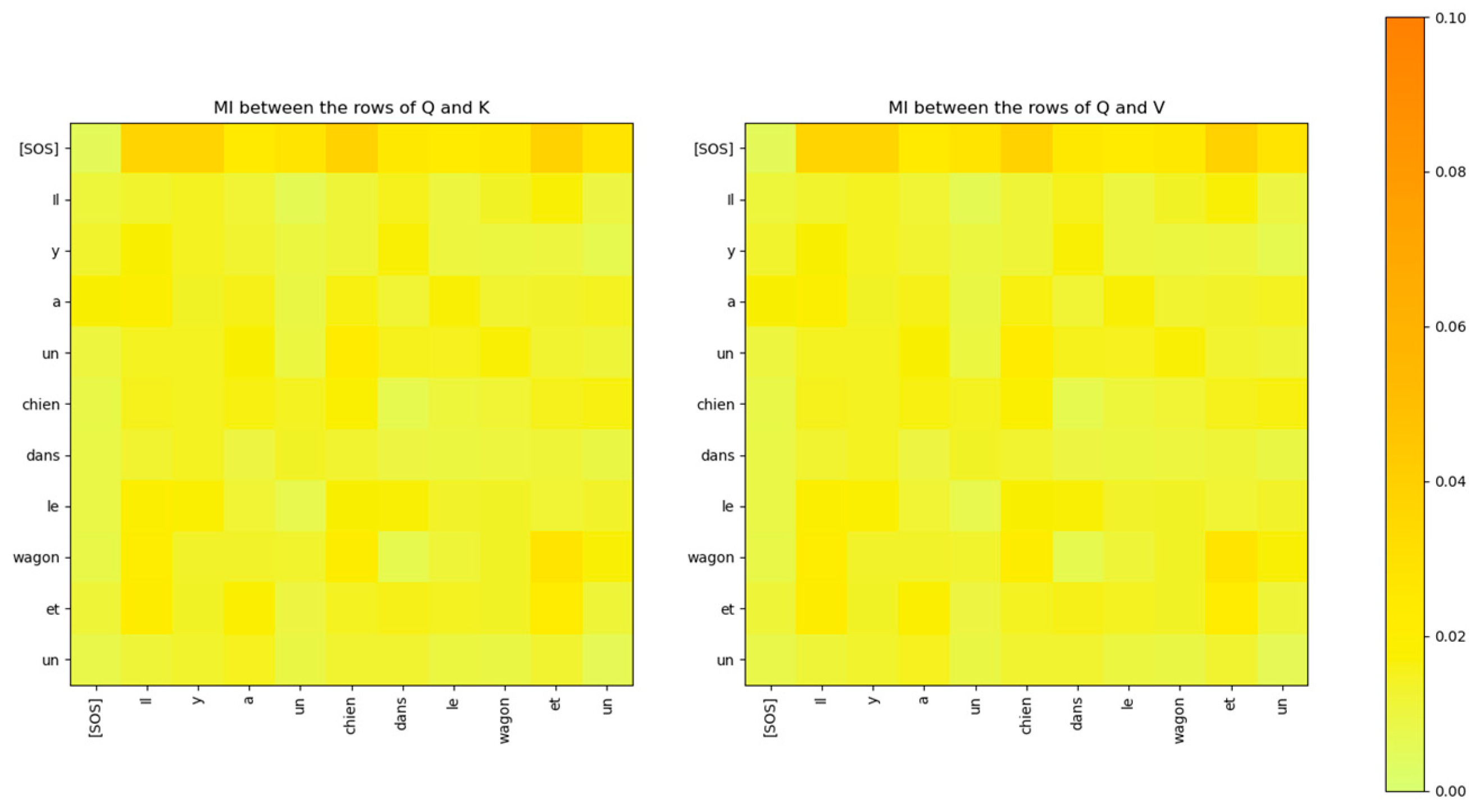
Figure 31.
The Mutual Information between the rows of the input Q matrix of the cross-attention layer of the decoder and the rows of the input K and V matrices from the encoder is low.
Figure 31.
The Mutual Information between the rows of the input Q matrix of the cross-attention layer of the decoder and the rows of the input K and V matrices from the encoder is low.
Figure 32.
Comparison of the Mutual Information between the Q and K heads (left) and the attention scores (right) for attention layer 2, head 2 of the decoder. The two matrices show similar relationships between the words of the sentence. However, the MI matrix exposes weaker relationships that are not visible in the attention scores matrix.
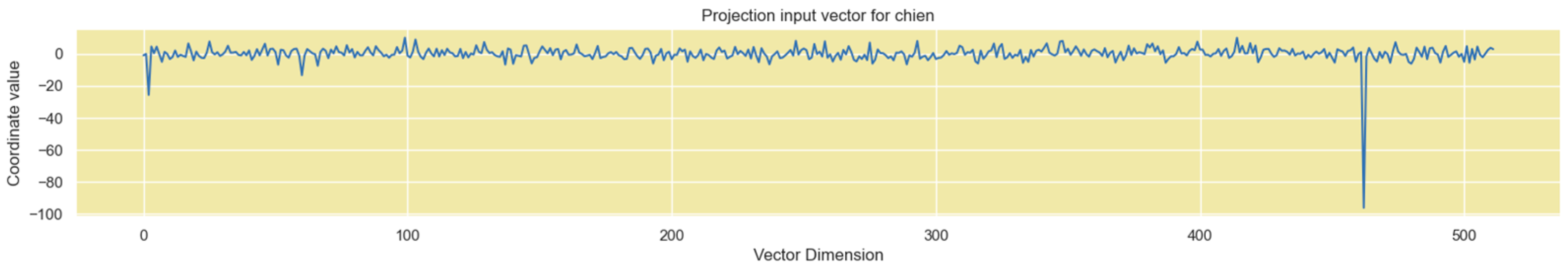
Figure 33.
Projection input vector has a single high coordinate value in dimension 461. All other dimension coordinates have low values.
Figure 33.
Projection input vector has a single high coordinate value in dimension 461. All other dimension coordinates have low values.
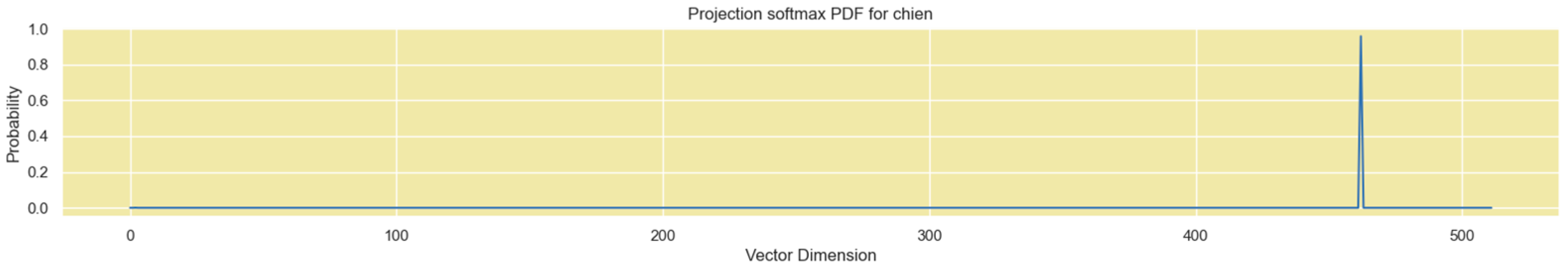
Figure 34.
Boltzmann probability distribution of the Projection vector input.
Figure 34.
Boltzmann probability distribution of the Projection vector input.
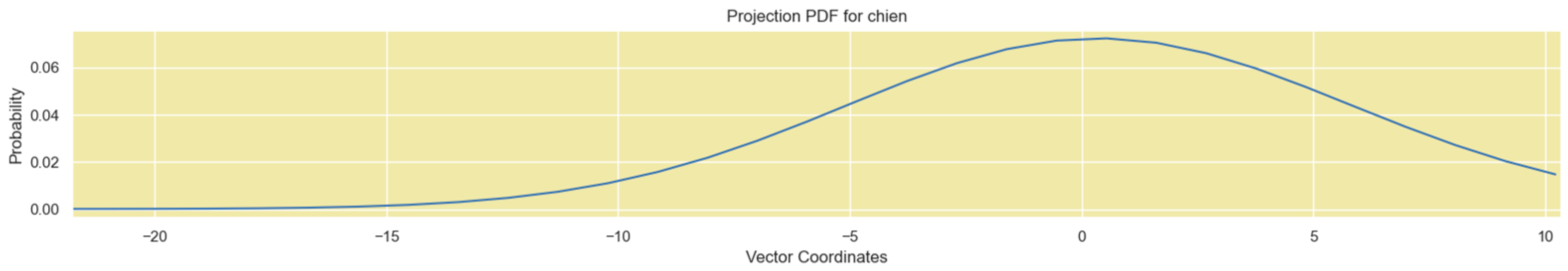
Figure 35.
The distribution of the other coordinate values of the Projection vector has a Gaussian shape.
Figure 35.
The distribution of the other coordinate values of the Projection vector has a Gaussian shape.
Figure 36.
Mutual Information between the Embedding output vectors for . Embedding vectors for different tokens are not completely mutually independent.
Figure 36.
Mutual Information between the Embedding output vectors for . Embedding vectors for different tokens are not completely mutually independent.
Figure 37.
Mutual Information between the Input Embedding output vectors for . The embedding vectors for different tokens are not mutually independent.
Figure 37.
Mutual Information between the Input Embedding output vectors for . The embedding vectors for different tokens are not mutually independent.
Figure 38.
Comparison of the statistical separation of vector coordinate distribution for the same word vector across multiple attention heads for and . The statistical separation is smaller with .
Figure 38.
Comparison of the statistical separation of vector coordinate distribution for the same word vector across multiple attention heads for and . The statistical separation is smaller with .
Figure 39.
Comparison of the MI and Wasserstein distance between the vector coordinate distribution across multiple attention heads for and . The figures show that the MI between the distribution across multiple attention heads is reduced with the reduced dimension model. Also, the distance between the coordinate distributions increased with the reduced dimension model.
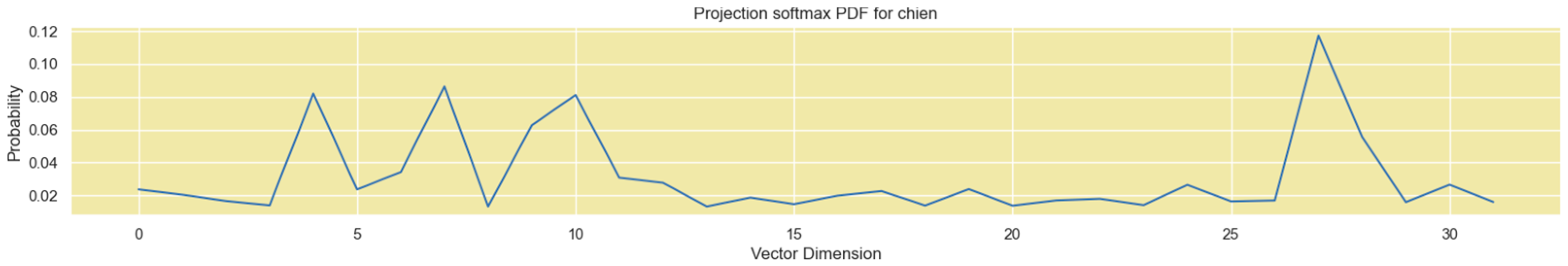
Figure 40.
Boltzmann probability distribution of the Projection vector input for . The impaired model shows that there are several dimensions with relatively high probability values, which will reduce the confidence of the softmax probabilities at the projection layer output.
Figure 40.
Boltzmann probability distribution of the Projection vector input for . The impaired model shows that there are several dimensions with relatively high probability values, which will reduce the confidence of the softmax probabilities at the projection layer output.
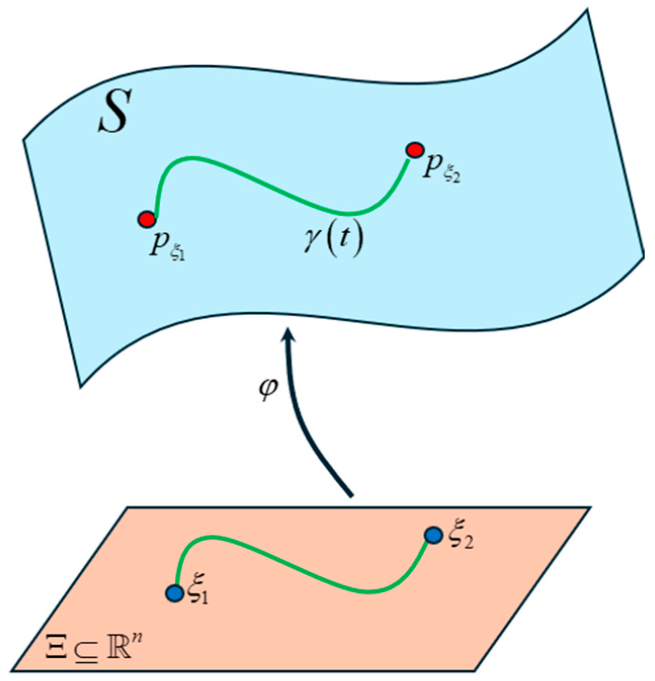
Figure 41.
Statistical manifold where each point is a probability distribution of the Transformer word vectors. Our goal is to find the shortest curve (i.e., geodesic) that connects these points.
Figure 41.
Statistical manifold where each point is a probability distribution of the Transformer word vectors. Our goal is to find the shortest curve (i.e., geodesic) that connects these points.
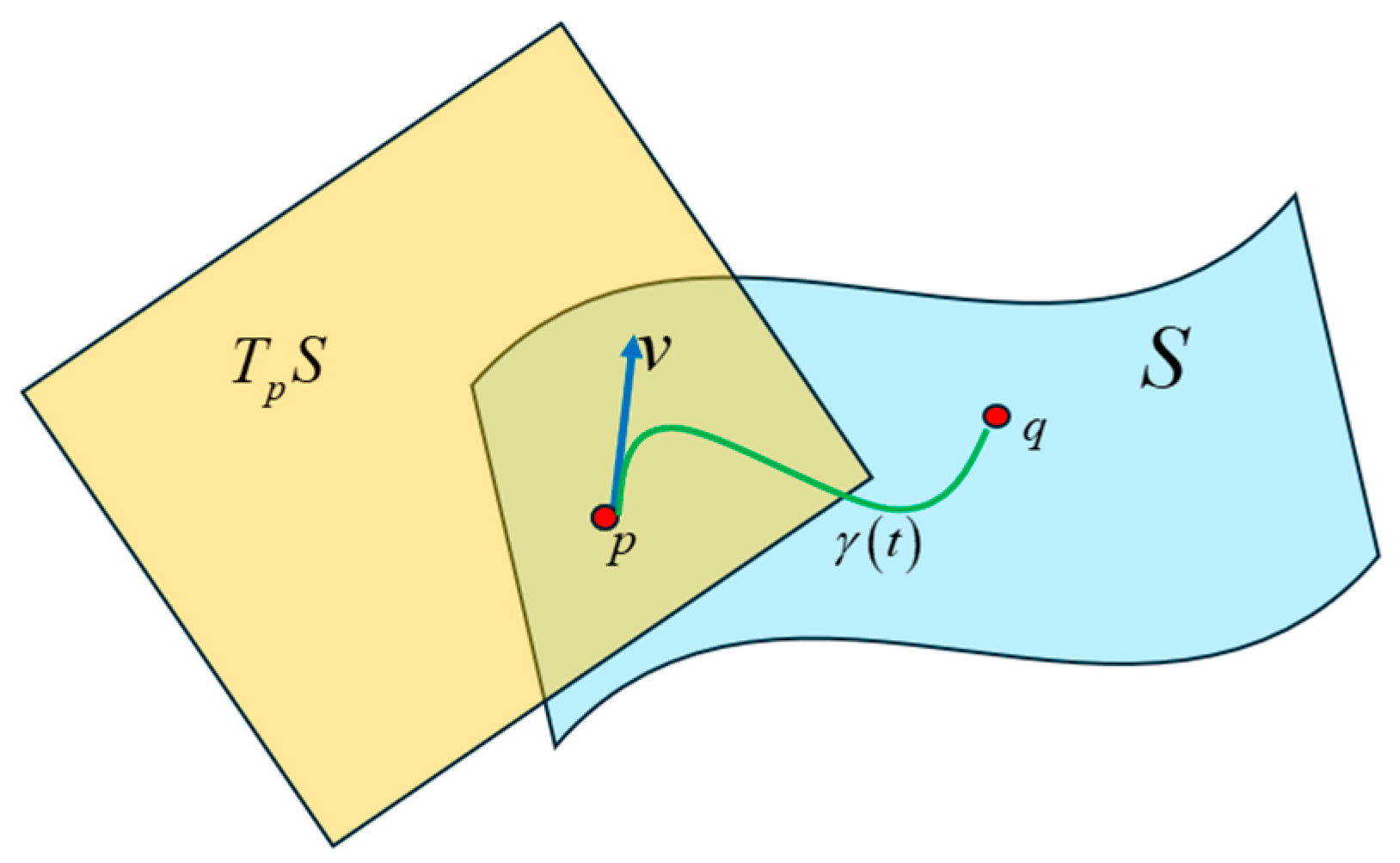
Figure 42.
A tangent space defined at the point p on the manifold and the tangent vector v lies in this space. This vector is tangent to the curve at point p.
Figure 42.
A tangent space defined at the point p on the manifold and the tangent vector v lies in this space. This vector is tangent to the curve at point p.
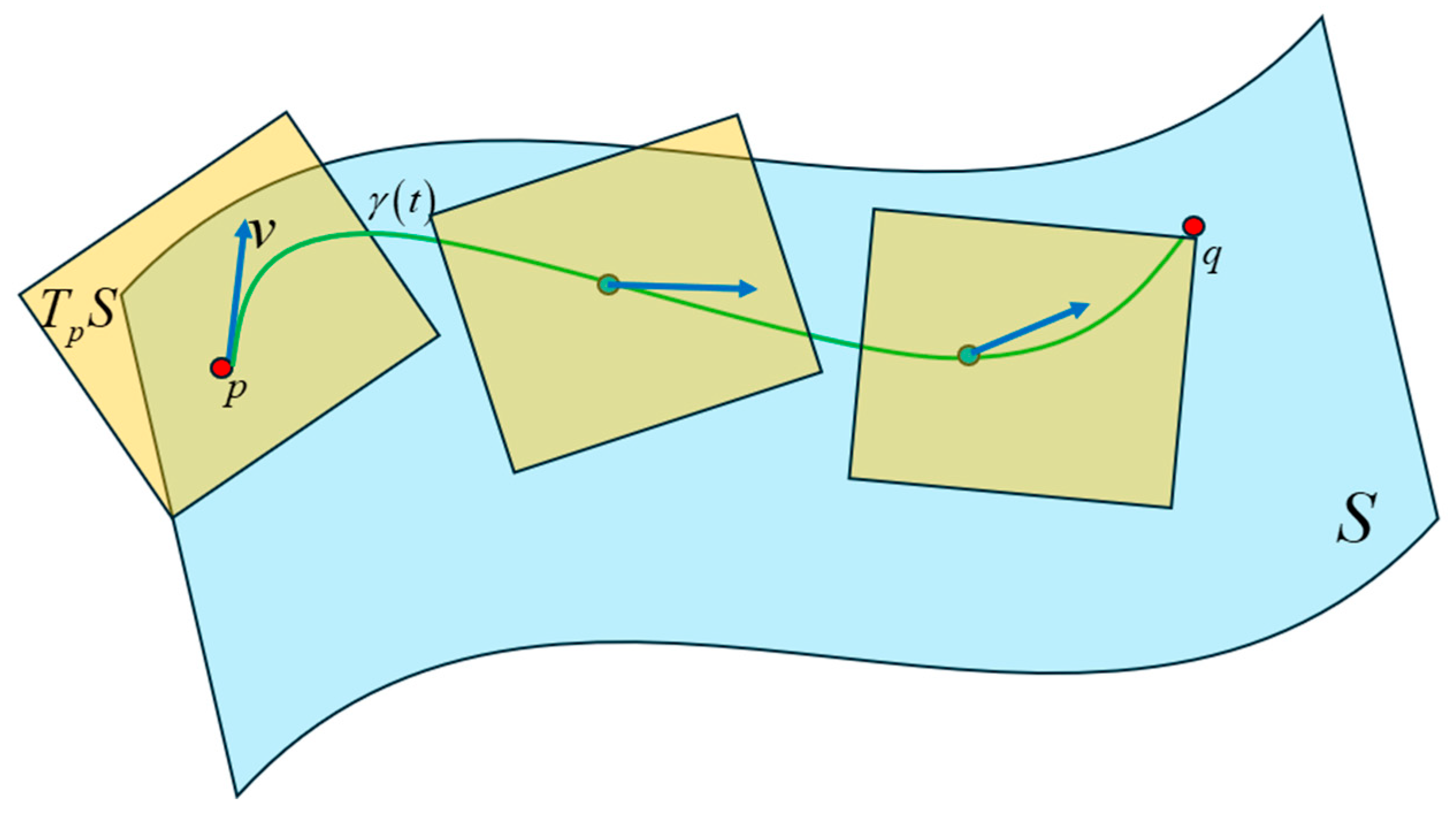
Figure 43.
A tangent space is defined at each point on the curve on the Riemann manifold by taking the derivative at that point. The tangent vector at each point lies in the tangent space at that point. Each tangent space is connected with an affine connection called the Levi-Civita connection. The Christoffel symbols are the connection coefficients for the Levi-Civita connection and describe how the basis vectors of the tangent spaces change throughout a coordinate system.
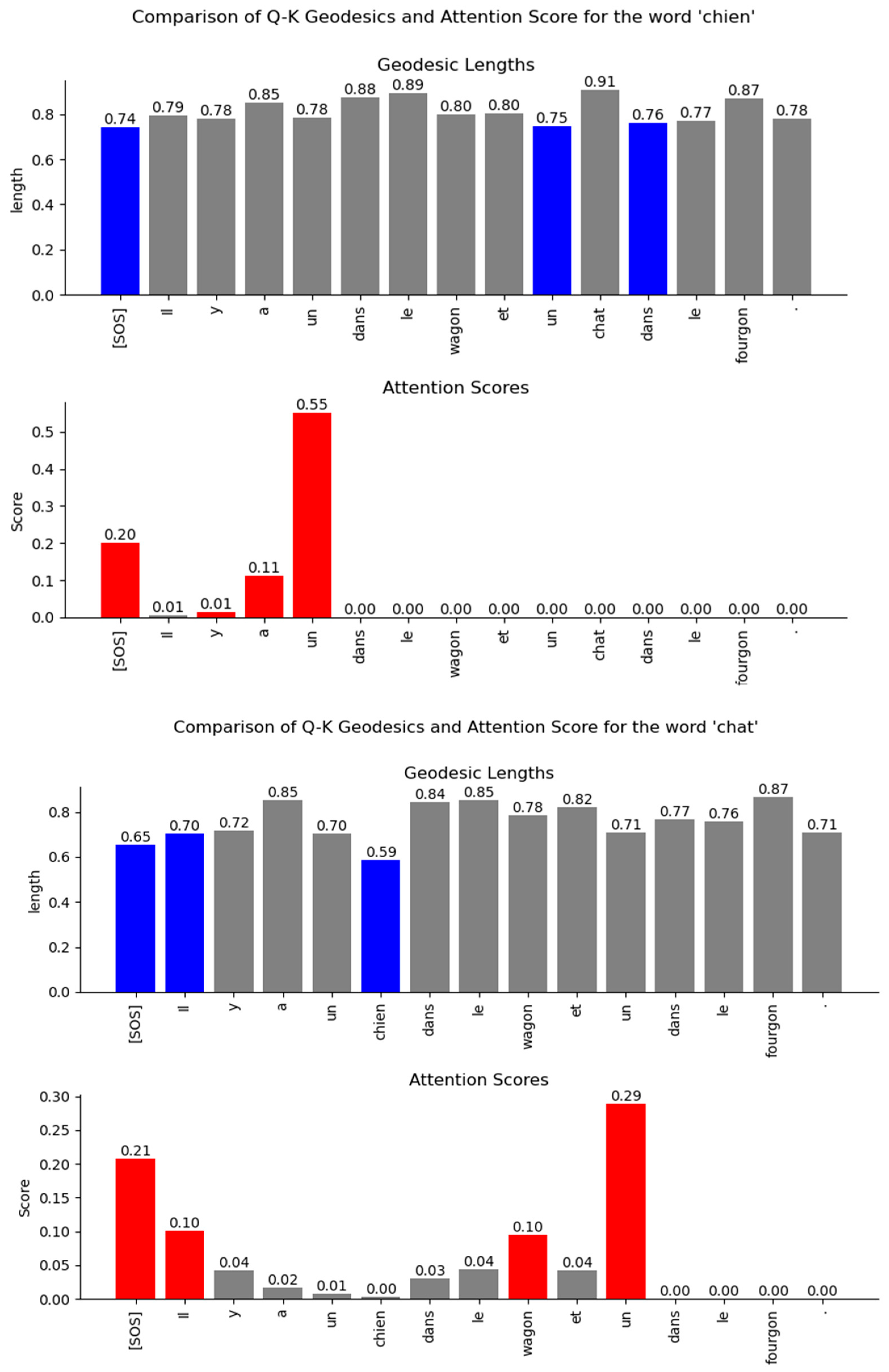
Figure 44.
Comparison of the geodesic lengths between the Encoder’s word vector distribution and the attention scores for specific words. The comparison is shown for layer 0, attention head 0. The smaller the value of the geodesics in the high-dimensional Riemann manifold, the stronger the relationship between the words. The bars in blue mark the lowest three geodesic values, while the bars in red highlight the highest three attention scores. The relationships inferred from the length of the geodesics are similar to the attention scores. The geodesic lengths expose additional relationships between the words that are not visible in the attention score plots.
Figure 45.
Comparison of the geodesic lengths between the Decoder’s word vector distribution and the attention scores. The comparison is shown for layer 0, attention head 0. The smaller the value of the geodesics in the high-dimensional Riemann manifold, the stronger the relationship between the words. The bars in blue mark the lowest three geodesic values, while the bars in red highlight the highest three attention scores. The relationships inferred from the length of the geodesics are similar to the attention scores. The geodesic lengths expose additional relationships between the words that are not visible in the attention score plots.


