1. Introduction
Jaynes popularized the entropy maximization technique as a powerful modeling tool for working with finite systems, where results like the Central Limit Theorem or the Stirling Approximation are neither necessary nor appropriate [
1,
2,
3]. On the basis of Jaynes’ work, this survey is designed to highlight some selected aspects of the technique that have appeared over the last thirty years, particularly driven by biological insights in parallel with more traditional topics from physics. Our examples are chosen to be as simple as possible, while still illustrating the key points we wish to convey. In particular, we avoid any reprise of the dependence of entropy and randomness on computational complexity or instrumental resolving power, as discussed in [
4]. Further details may be found in the cited references and their bibliographies, but there are many opportunities for interested readers to continue the development and refinement of the topics that we raise.
In
Section 2, we set the framework for most of the paper by revisiting the very well-known Gibbs Canonical Ensemble. In particular, we draw attention to an important but rarely mentioned subtlety, namely the strength of the inequality constraints in the procedure of entropy maximization by the method of Lagrange multipliers (
7). For perspective,
Section 3 takes a brief look at the alternative game-theoretic approach adopted by Topsøe and his school (cf. e.g., [
5,
6,
7]). We propose a biological interpretation for the game as ecological co-evolution between a pair of species: predator and prey. The prey’s interest in randomizing the interactions with the predator, and the predator’s interest in regularizing those interactions, exactly capture the roles of the two players in the abstract game. Thus, the issue,
“The sense in assuming that Player I has the opposite aim, namely to maximize the cost function is more dubious”.
Ref. [
5] (p. 198) is resolved by assigning the role of Player I to the prey and Player II to the predator. In this interpretation, the cost function measures how long it will take the predator to determine the prey’s strategy for escape from pursuit.
Section 4 reviews the standard interpretation of the entropy maximization approach to the Canonical Ensemble within statistical mechanics, where macrostates
are identified by respective energies
. In preparation for the subsequent application to a phase transition in an ecological system (
Section 6), we go one step beyond Baez’ advocacy of the Lagrange multiplier
as a “coolness” parameter [
8] in preference to the temperature
T, arguing instead for
, the negative of the coolness
, as the best choice. Certainly, the temperature
T is ill-suited to treatment of condensed matter situations where energies of states are bounded both below and above (e.g., in quantum optics, cf. [
9,
10]). The use of
as a coordinate in condensed matter physics [
9] (Figure 2) then naturally leads to our preference for
, whose increase is subsequently seen to concur with the Arrow of Time. Compare (
27) with (
31), for example.
Section 5 uses the Canonical Ensemble for the analysis of an ecology,
Lake Gibbs, where species
with respective natural growth rates
compete within an environment having a fixed carrying capacity of
N individuals. This system provides a macroscopic model of Eigen’s phenomenological rate equations [
11]. While the equations may be solved using standard techniques for handling ordinary differential equations (ODEs), starting from known initial conditions [
12,
13], the entropy maximization technique offers a novel approach to the solution of the system of coupled ODEs, without the need for initial conditions [
14]. This feature of the entropy maximization technique is especially relevant for biological applications, where one encounters existing systems whose genesis is uncertain: the classic “chicken-and-egg” dilemma!
At first glance, use of the Canonical Ensemble in biology may appear to be unrelated to the classical use case of statistical mechanics. However, following the lead of the particle physicists in using natural units with Planck’s constant set to 1 [
15] (§III.2), the energies
that appear in the statistical mechanics applications of the Canonical Ensemble are seen to have the dimensions of inverse time, exactly like the growth rates
that appear in the ecological application. Thus, our preferred conjugate Lagrange multiplier
becomes directly identifiable as an emergent time parameter, sharing the statistical macroscopic nature of temperature. As
increases, the ecology of Lake Gibbs ages by moving from a diverse mix of the species
towards an unhealthy monoculture dominated by the most prolific species
r—compare (
1). The ecology could be rejuvenated by restocking the lake with a broad variety of species, thereby resetting the emergent system time
back to a lower value.
Section 6 extends the entropy maximization treatment of the Lake Gibbs ecology: not only to cover the constrained phase analyzed in
Section 5, but also the earlier unconstrained phase where each species
i (for
) is growing exponentially at its natural, unchecked pace
, before the carrying capacity of the lake is reached [
16]. Thus, entropy maximization is shown to handle a phase transition, for a finite system, without resort to any infinite “thermodynamic limit”. This is achieved by moving beyond the strict inequalities for the constraints on the optimization domain noted in
Section 2. Along with positivity constraints for parameters
tracking the respective species
, an
order parameter subject to a weak non-negativity constraint is added (
38). If the constraint is binding, i.e.,
, then the entropy maximization reduces to its previous form for the constrained phase as described in
Section 5. On the other hand, if the constraint is slack, i.e.,
, then the entropy maximization returns the unconstrained phase where each species is growing exponentially. As a proof of concept, this basic example suggests that future research, working with richer constellations of strong and weak inequality constraints, should provide finitary entropy maximization analyses of more elaborate, multidimensional phase diagrams.
2. The Canonical Ensemble
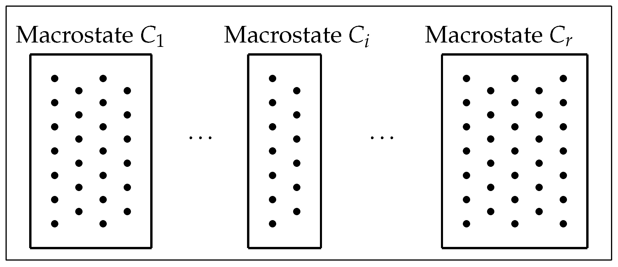
Consider a finite, nonempty set or
phase space (
Figure 1) that comprises
N equally likely individual elements or
microstates (dots in
Figure 1) with a partition
into the disjoint union of a family of
r subsets or
macrostates (boxes in
Figure 1). Suppose that the macrostate
comprises
microstates, for
, so that
The set
of (
2) may be considered as (invoking) an
experiment: take a microstate and determine the macrostate
to which it belongs.
Figure 1.
A phase space of microstates, with a partition
into macrostates [
17] (Figure 2).
Figure 1.
A phase space of microstates, with a partition
into macrostates [
17] (Figure 2).
What information is gained by performing the experiment? Initially, a store of size
would be required to tag the microstates. Suppose that we perform the experiment and obtain outcome
. In that case, knowing that the microstates are localized within
, we now only require a store of size
. The information gain as a result of the experiment is
. However, there is only a probability
of obtaining outcome
. The expected information gain from the experiment is the weighted average
of the information gains from each of the possible outcomes. This quantity is described as the (information-theoretic)
entropy of the partition
. It may be characterized as the expected value of the logarithm of the odds, namely
to one, of obtaining a particular macrostate
.
In practice, the specific partition of the phase space into macrostates is not known a priori. However, suppose that a numerical value (typically representing a dimensioned scientific quantity like an energy or a growth rate) is associated with each macrostate. A particular macrostate
then consists of all those microstates that yield an observed numerical value
when the experiment is performed. While the actual probabilities
of the individual macrostates may be unknown themselves, suppose that the expected outcome
is known, say from a measurement performed on a sample of the microstates. In order to construct a model, the probabilities
have to be assigned. If the expected value (
6) is the only information available, then the truest model is the one that maximizes the entropy
subject to the constraint (
6). This model is known as Gibbs’
canonical ensemble.
The maximization problem is usually solved by the method of Lagrange multipliers [
18] (Th. 3.2.2). Here, we wish to draw attention to a subtle detail of the procedure, which is rarely stated explicitly: the nonemptiness of the macrostates in the family (
2) means that the optimization is taken over the set
of
positive probabilities, the interior of the
-dimensional simplex
. Thus, in maximization of the Lagrangrian
the stationarity conditions
for all
apply since the maximization is performed over
. They give
or
Substitution in the completeness constraint from (
3) yields
or
Defining the
partition function (or “Zustandsumme”)
of
, we have
in Gibbs’ canonical ensemble. The entropy (
5) may be written as
in terms of the variable
. As another point worthy of special attention, we emphasize that the units for the multiplier
are inverse to those for the numerical values
.
3. The Game Theoretic Approach
While the entropy maximization procedure outlined in the previous section has a number of advantages, most notably the identification of the Lagrange multiplier
as a conjugate to the numerical values
assigned to the macrostates, it is not the only approach. The Danish school (cf. [
5,
6,
7], for example) have strongly advocated for an approach that involves a game between two players. In their version,
Player I chooses a consistent distribution, and Player II chooses a general code. …[T]he objective of Player II appears well motivated. [A] cost function can be interpreted as mean representation time, …and it is natural for Player II to attempt to minimize this quantity. The sense in assuming that Player I has the opposite aim, namely to maximize the cost function, is more dubious. [
5] (p.198).
Here, in our simplified setting, which is chosen to avoid detailed topological and analytical concerns, we present a brief and introductory alternative account that is founded upon a more adequate, symmetrical notation and a representative interpretation of the two respective Players I and II as prey and predator in an ecological context. A parallel interpretation in a political science context might identify “people” and “government” as the two players. A relationship of this kind is implied, for example, in the work of J.C. Scott [
19,
20]. We refer to our description as the
Predator–Prey Representation.
The ecological principle underlying the Predator–Prey Representation is that predators must seek to regularize their relationships with their prey, while the prey seek to randomize those relationships. To catch their prey, predators need encoded hunting strategies. But to evade their predators, the prey need unpredictable escape strategies.
In the model, the prey may draw from a set
of so-called
consistent probability distributions
on a set of evasive actions that includes no more than a finite number
r of elements. Thus, a consistent distribution gives a specific option for an escape strategy.
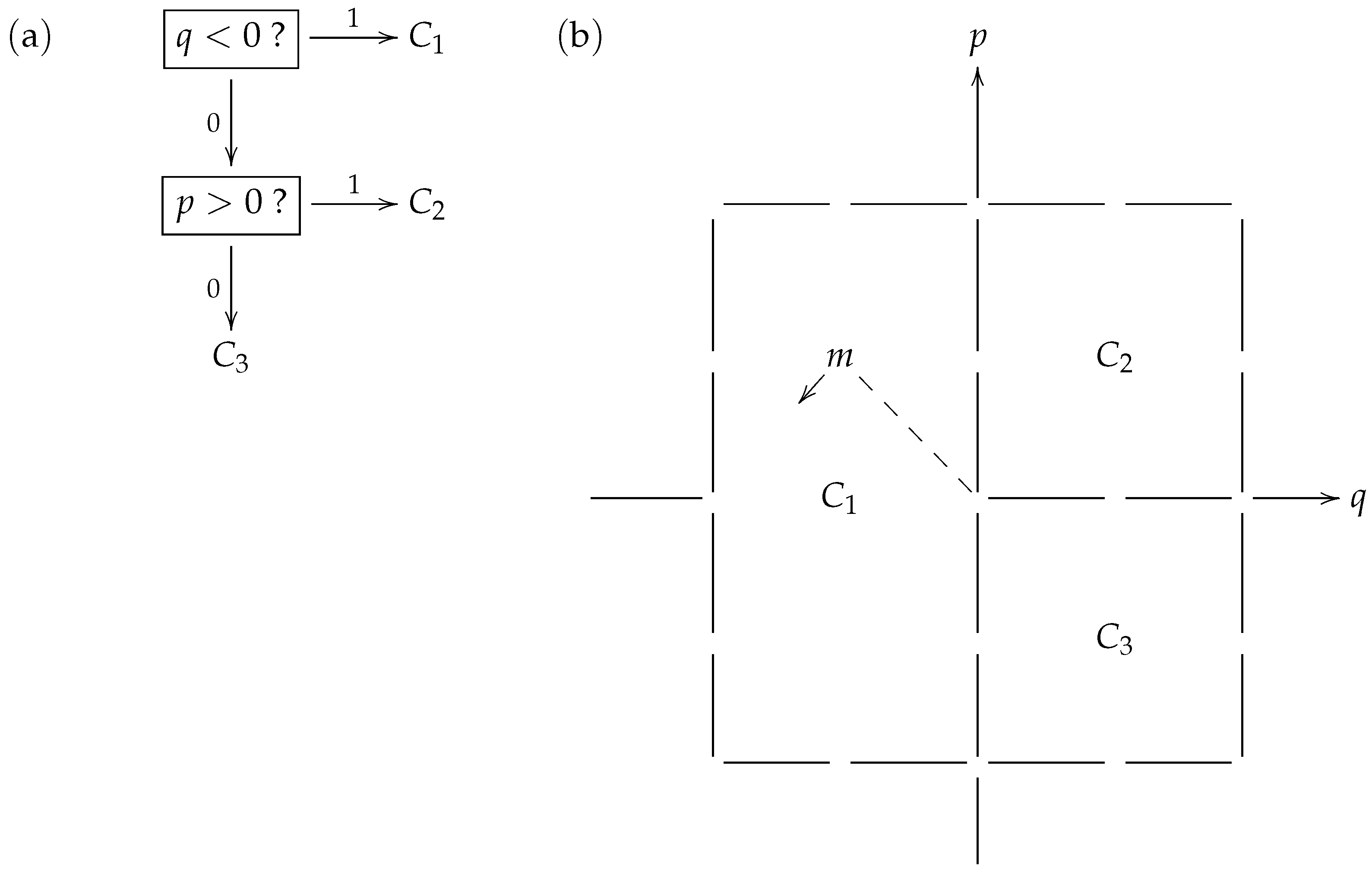
Figure 2 shows a toy model strategy where the prey is aiming to distract its predator when being pursued from behind, by swinging its tail in a pendulum-like motion. In
Figure 2b, the particular consistent distribution
exhibited is related to (and identified with) a macrostate partition
of the type of phase space displayed in
Figure 1. Furthermore, the phase space in this particular example may be overlaid on the classical phase space of a linear harmonic oscillator (such as a pendulum) with position variable
q and momentum variable
p. Thus, a microstate (such as
m that appears in the macrostate
) may be considered to describe a brief video clip of a specific tail motion.
Table 1 identifies the macrostates with specific tail motion features that would be perceived by the predator in their encoding of the prey’s behavior, using the binary prefix code
displayed in
Figure 2a.
When applying the code
during the chase in its attempt to learn what the prey is doing, the predator first checks if the prey’s tail is on the left side (
). If the answer is “yes” or 1, the predator has taken just 1 step to correctly identify that the prey has selected macrostate
. This event occurs with probability
within the prey’s strategy
. On the other hand, if the answer is “no” or 0, so the tail is on the right, the predator then checks if the prey’s tail is swinging to the right (
). If the answer to this question is “yes” or 1, the predator has taken 2 steps to correctly identify that the prey has selected macrostate
, an event that occurs with probability
within the strategy
. Finally, if the answer to the latter question is “no” or 0, the predator has taken 2 steps to correctly identify that the prey has selected macrostate
, an event that, again, occurs with probability
within strategy
. Thus, with the code
, the expected number of steps that the predator takes to recognize the prey’s strategy
is
matching the entropy
of the consistent distribution
in bits.
In the “bra-ket” notation that appears on the left of (
14), we switch the sides relative to [
5] (p.196) and [
7] (8) so that the distribution
belonging to Player I (the prey) appears first, while the code
belonging to Player II (the predator) appears second. In general, for a code
with respective code lengths
and a consistent distribution
with respective probabilities
, the
cost function
is defined. As seen on the basis of the illustrative example from
Figure 2, the cost function represents the expected time (number of questions asked and answered) taken for Player II using a binary prefix code
to recognize which macrostate has been chosen from the canonical distribution
adopted by Player I. The abstract information-theoretic game between Player I and Player II, as envisaged by the Danish school, is instantiated by the concrete ecological games that take place over multiple generations as prey and predator population pairs co-evolve. In particular, the problem raised in the earlier quotation from [
5] (p. 198),
“The sense in assuming that Player I has the opposite aim, namely to maximize the cost function is more dubious”,
is clearly solved by the prey’s interest in extending the time it takes its predators to identify an escape strategy.
The full set of escape strategies
available to the prey is identified as the set
of consistent distributions. Now, consider a particular code
available to the predator as a hunting strategy. The
risk [
5] (3.11)
associated with that hunting strategy expresses the maximum length of time it might take the predator to identify the prey’s behavior using
—a measure of the predator’s risk of starvation if it were to stubbornly rely on
as its hunting strategy. Successful predators deploy multiple hunting strategies, assembled in a set
of codes
. Their risk of starvation is reduced to their
minimum risk value [
5] (3.12)
if they are able to draw on any one of these strategies.
Dually, we begin by noting that the full set of hunting strategies
available to the predator has been identified as the set
of codes. We may now consider a particular consistent distribution
that is available to the prey as an escape strategy. The
coded entropy(cf. [
5] (3.9)) associated with that escape strategy expresses the minimum length of time it might take a predator to identify the strategy—a measure of the prey’s risk of capture or randomization success—if it were to stubbornly rely on
as its escape strategy. Successful prey species deploy multiple escape strategies, assembled in their repertoire
. Their time of freedom when pursued is maximized to the
maximum coded entropy
if they are able to draw on any one of these strategies (cf. [
5] (3.10)).
Taking infima over
on each side of the quantified statement
gives
. The inequality
then follows on taking the supremum over
. It provides the final link in the full chain
of inequalities that summarizes the relationships between the behaviors of the prey and the predator. Reference [
5] continues with a general abstract analysis of when equality is obtained. In the ecological setting, equality is to be expected for stable predator–prey population pairs that have co-evolved over multiple generation times.
4. Statistical Mechanics
After the brief excursion into the game-theoretic approach, we return to a consideration of the Lagrangian approach as presented in
Section 2. In the classical applications of the canonical ensemble, one may consider the microstates as particles having a certain energy. Thus, the numerical value
associated with macrostate
is an energy (say in joules). The conjugate variable
, which was carefully chosen to match the non-classical applications in the subsequent sections, is connected to the temperature
T (say in degrees Kelvin) by
using Boltzmann’s constant
k. Baez [
8] (p. 30) refers to the traditional conjugate variable
as the
coolness: the lower the (non-negative) temperature
T, the higher the value of
. The problem with such traditional conventions, even within statistical mechanics, is that they are ill-adapted to handling
negative temperatures, which are readily observed in condensed matter situations where energy levels are bounded both below and above [
9,
10]. In particular, the use of
(i.e., our
!) as an abscissa coordinate in the first figure of [
9] should be noted. If
and
are avoided, (
22) shows that an increase in
conveniently corresponds to an increase in
T, and
vice versa.
The relation (
22) gives some insight into the nature of the quantity
in the canonical ensemble: Just like the temperature, it is a statistical property of collections of microstates. The
thermodynamic entropy is
in joules per Kelvin degree. The
thermodynamic potential is the dimensionless quantity
while the
Helmholtz free energy is
in joules. The relation (
13) takes the form
The Equation (
12) becomes
a well-known formula of kinetic theory (compare [
21]). For example, it may be used to describe the distribution of atmospheric particles at different heights, according to their potential energy in the Earth’s gravitational field [
21] (§40-1,2), [
3] (§6.1.2(a)).
When considering physical applications of the canonical ensemble, it may prove useful to use
natural units or
Planck units with Planck’s constant set to 1 [
15] (§III.2). Then, the energies that appear in the statistical mechanics applications of the Gibbs ensemble are seen to have the dimension (time)
−1. For example, the energy of a photon of light is given as the product of Planck’s constant with the frequency of the corresponding wave.
5. Time Emergence
In the statistical mechanical applications of the canonical ensemble discussed in
Section 4, the coolness
, a Lagrange conjugate of energy, emerges as a statistical property of a collection of microstates. On the other hand, using natural units, such Lagrange conjugates of energy as
or our preferred
should appear with the units of time. Now, following [
14], we examine a model where
does indeed represent an emergent intrinsic age of a biological system. It provides a conceptually instructive model of competition between
r different species, labeled
, as described by Eigen’s phenomenological rate equations [
11]. Suppose that species
i has an unconstrained growth rate of
(say in
per annum units). This means that a population of
individuals of species
i growing without constraint has a rate of change
(using Newton’s dot notation for the derivative). At a Newtonian time
t in an interval
from a start time
s to an ultimate time
u, the population
is given as
—exponential growth. Competition (as modeled by Eigen’s equations) arises when the individuals of the
r species form a joint population maintained at a constant total count
N. The birth of one individual is compensated for by the death of another.
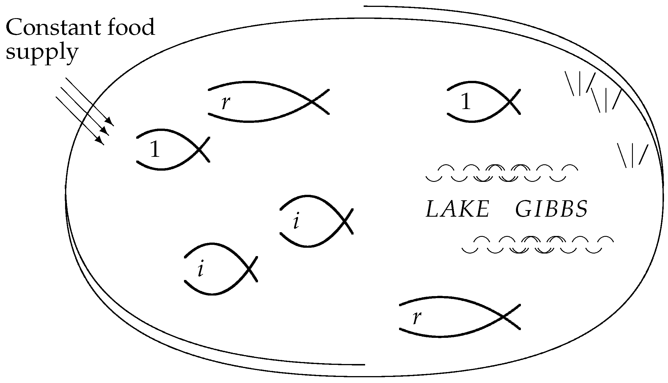
Figure 3 visualizes the individuals as fish in a lake, where the food requirements of each individual fish are the same, and the food supply sustains the constant total number
N.
Figure 3 may also be viewed as a slightly less abstract version of
Figure 1. The individual fish correspond to the microstates, which share a macrostate if they belong to the same species.
The traditional treatment to determine the population
of species
i at given Newtonian times
t in an interval
(cf. [
12,
13] or [
16] (§4)) involves solving the coupled quasilinear system
of ordinary differential equations. Although (
26) may be seen as a special case of [
3] (20 Equation (80)), the treatment in that reference, concerned as it is with equilibrium or long-term values, does not relate to our analysis, the coupling being introduced through the final, quadratic or two-point interaction term of (
26). Based on an Ansatz to translate to a linear system [
16] (26), the classical solutions
are valid over the Newtonian time interval
. Here, the initial conditions that are required to solve the system of ordinary differential equations record the population count
at
.
The function
appearing in the middle part of (
26), whose specification follows from
represents the instantaneous
cull rate
required to hold the total population constant at the carrying capacity
N. The argument
of the exponential in the denominator of the right hand side of (
27) is then recognized as counting the total number of starvation victims registered over the time interval
.
In the approach through the canonical ensemble, we imagine going to the lake and catching a moderately sized group of fish in a net. The relative frequency
of each species
i in the catch is taken as a good approximation to the overall probability
of catching a member of that species. In other words, we take
for
at any given time. Knowing these relative frequencies
, together with the unconstrained growth rates
of each species, we obtain the expected average value (
6) that is the premise for the canonical ensemble. The relationship (
28), fundamental to our approach, equates the cull rate
E to the average
or
gross growth rate (GGR) of the population. Equation (
12) yields
in particular with
as an initial condition that does not need to be specified separately in our approach. When the species are labeled by increasing unconstrained birth rates (assuming non-degeneracy), say
with
, then the most prolific species
r will ultimately dominate.
The intrinsic time
that appears in (
31) is an emergent statistical property of the complex system. As the system ages, the proportion of the dominant species
r increases, leading to a lack of biodiversity. Restocking the lake with a good mix of the various species would rejuvenate the ecosystem, resetting the system time
independently of the relentless forward progress of the Newtonian time
t.
In conjunction with the emergence of the system time
, the canonical ensemble treatment of the ecosystem with the fixed carrying capacity
N has an additional feature, which will be exploited more in the following section. For this discussion, assume the start time
s is set to
, with a uniform distribution at that time in which each species
i has a population
Then, the solutions (
25) of the unconstrained Equation (
24) for a negative time
t take the form
Let
M denote the total fish population at any given time. Thus,
for
, while Equation (
35) gives
for
. As a consequence, the equations
for the relative frequencies, obtained for a positive time
t from (
12) making use of the canonical ensemble description of the constrained ecology, are equally valid during the unconstrained population growth at negative times. It is indeed remarkable that the relative frequencies extrapolate backwards from the canonical ensemble, even though the assumptions leading to the canonical ensemble do not apply in this unconstrained regime.
6. A Phase Transition
In the classical entropy-maximization treatment of the canonical ensemble (
Section 2), the optimization is taken over the open set
(
7) of
positive probabilities, the interior of the
-dimensional simplex
. In the competition model presented in
Section 5,
represents the probability of catching a fish of species
i, for
, although we often prefer to use the relative frequency
of (
29) as a proxy. In this section, following [
16], we now consider an additional variable
and the subset
of the
r-dimensional simplex
, maximizing the
parametric entropy
over the non-open set
. This procedure leads to a more complete description of the ecology depicted in
Figure 3 that also applies to the
unconstrained phase where the total fish population
M is below the carrying capacity
N. In this broadened context, the regime analyzed in
Section 5 is called the
constrained phase. For simplicity of exposition, the phase transition is assumed to take place at system time
with a uniform distribution of all the species at that time, as in (
34) above. Following the analogy between time and temperature, one might regard setting the time of the phase transition to zero as analogous to the (pre-1948) Celsius scale setting of zero for a phase transition of water.
Given the various kinds of phase transition that physicists might recognize, we invoke Penrose’s general definition [
22] (§28.1),
“A phenomenon of this nature, where a reduction in the ambient temperature induces an abrupt gross overall change in the nature of the stable equilibrium state of the material, is called a phase transition”,
to justify our current terminology. In the ecological setting, a “reduction in the ambient temperature”
T is interpreted as an increase in the system time
in accordance with the relation (
22). Co-opting common physical terminology, we describe the variable
in (
38) as the
order parameter [
23]. Since the variables
no longer function directly as naive catch probabilities during the unconstrained phase, the way they do during the constrained phase, we refer to them as (additional)
parameters in the complete history of the ecosystem, thereby leading to the terminology of (
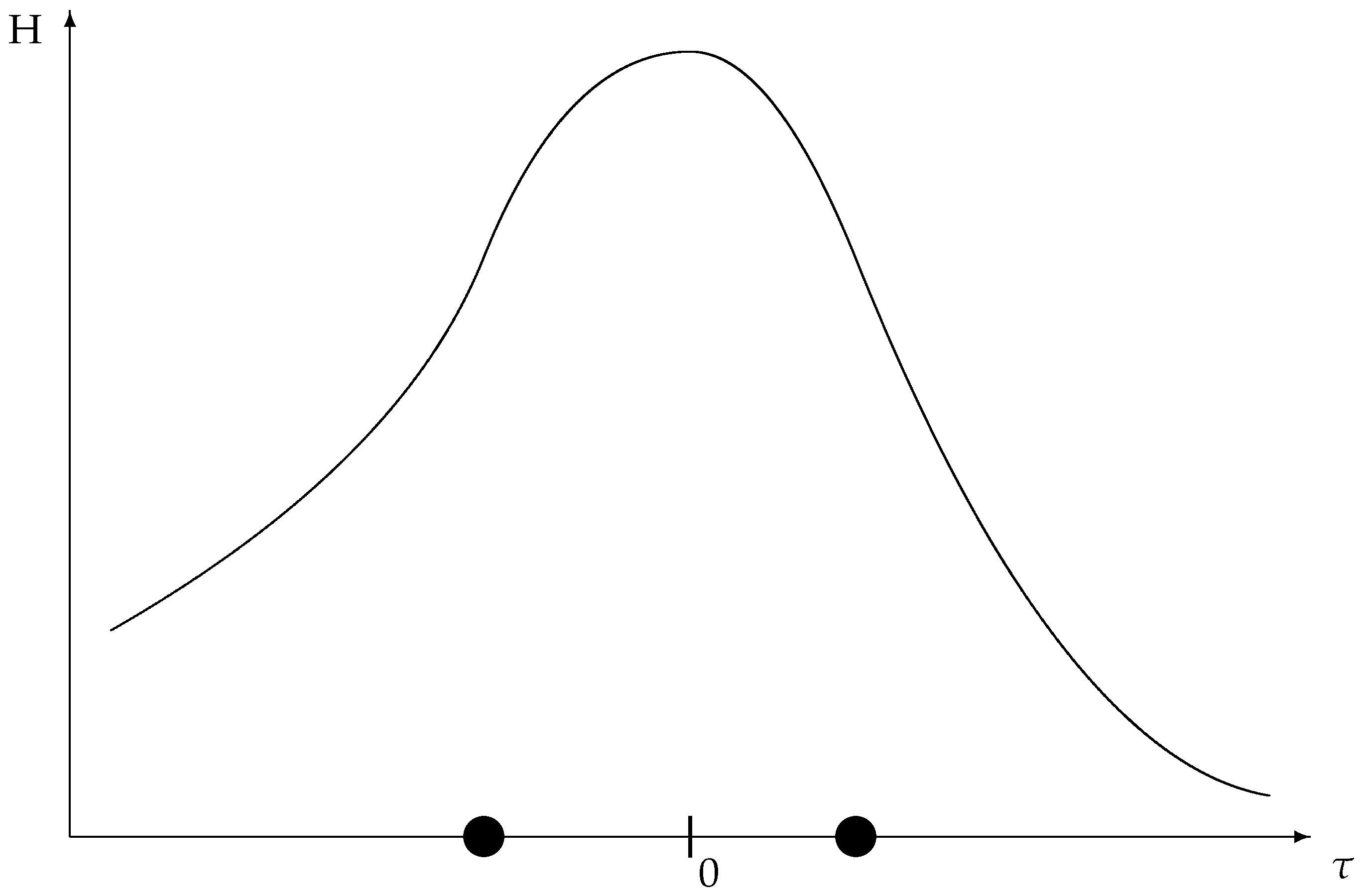
39) for the corresponding entropy. We then define
as the
population entropy (
Figure 4) to contrast with the parametric entropy of (
39).
Since the population counts of the various fish species do not undergo a discontinuous change at the phase transition, one may wonder where the “abrupt gross overall change in the nature of the stable equilibrium state” comes in. Mathematically, it is seen in the change from the exponential growth solution (
25) to the modified version (
27), where the denominator with the exponentiated integral suddenly appears. For the individual fish, it means the drastic arrival of the possibility of death by starvation, where previously they were always able to live out their natural lifespans. It is also worth noting the emergence of the “long-range correlations” indicated by the addition of the final term of (
26) to the original unconstrained growth Equation (
24).
Heuristically, if not too literally, the order parameter
may be associated with a
ghost species 0 having a natural unconstrained growth rate
. Consider maximization of the parametric entropy (
39) over the non-open set
of (
38) subject to the equality constraint
on the parameters. The quantity
D appearing in (
41)—obviously motivated as a version of (
6) that has been extended to include the ghosts—is discussed at the end of this section using (
51). We take the Lagrangian
in terms of the parameters
. When the weak inequality constraint on
from the definition (
38) of
is
binding or “active” [
18] (p 221), i.e.,
and
(either by convention or as the result of the limiting procedure
), we have
in terms of the original Lagrangian (
8). Thus, in the situation where the order parameter
is zero and the remaining parameters
are recognized as the corresponding relative frequencies, the extended description reduces to the original description. In particular, when
(i.e., there are no ghosts), the parametric entropy reduces to the population entropy.
When
, the weak inequality constraint on
from the definition (
38) of
is
slack or “inactive” [
18] (p. 221); the analysis of the Lagrangian (
42) for the parametric entropy proceeds in similar fashion to the analysis of the original Lagrangian (
8) in
Section 2. The stationarity conditions
for
reduce to
or
. A substitution in the completeness constraint yields
or
using (
11) for the latter term, yielding the expressions
for the parameters
.
For
, the expression (
43) determines the order parameter as
Taking Equation (
43) for
, the remaining parameters may be rewritten in the form
For
, a substitution of this expression into (
35) yields
whence (
36) may be rewritten as
to determine the total population in the unconstrained phase in terms of the order parameter. The assignment
represented by (
47) may also be inverted to yield
as an equivalent expression of
in terms of
M. It is clear that the expressions (
46) and (
47), valid for negative times, will not continue to hold in the constrained regime where
.
In the unconstrained phase, an experiment may be conducted to determine the total population (
47) and, thus, the order parameter as given by (
48). A fisherman trawls a fixed volume of water and counts the number
of fish caught in the trawl. The number of fish
that would be caught in the trawl at the carrying capacity
N is presumed to be known, so the total population
M is obtained as
. This refinement of the catch protocol is described as the
trawl. Using the relation (
45) that holds for
, the relative frequency of species
i in the trawl is
recalling (
37) for the first equality. The outer fragment
of (
49) is then seen to hold for the entire history, extending the previous identification
which only holds in the constrained regime
. The factor
appearing in (
50) is described as the
modifier for any
within the range
, and, thus, the parameters
are recognized as
modified relative frequencies.
The quantity
D that appears in the constraint (
41) may now be examined. We have
using the second equation of (
50). Since
D is given as the product of the modifier with the gross growth rate (
30), it is described as the
modified gross growth rate. In particular, once the order parameter is known from the trawl, then the modified GGR is obtained from the unmodified GGR, which is also determined from the trawl.
In summary, the extended Lagrangian
given in (
42) represents a maximization of the parametric entropy, subject to the completeness constraint on the parameters and the knowledge of the modified gross growth rate
D that is obtained from the trawl. When
is maximized over the constraint set
that includes a weak inequality for the order parameter
along with the usual strong inequalities for the remaining parameters, it enables one to use entropy maximization for the modeling of a phase transition in a finite situation without recourse to any infinitary “thermodynamic limit”.


