

Comparative Study on Flux Solution Methods of Discrete Unified Gas Kinetic Scheme


Abstract
1. Introduction
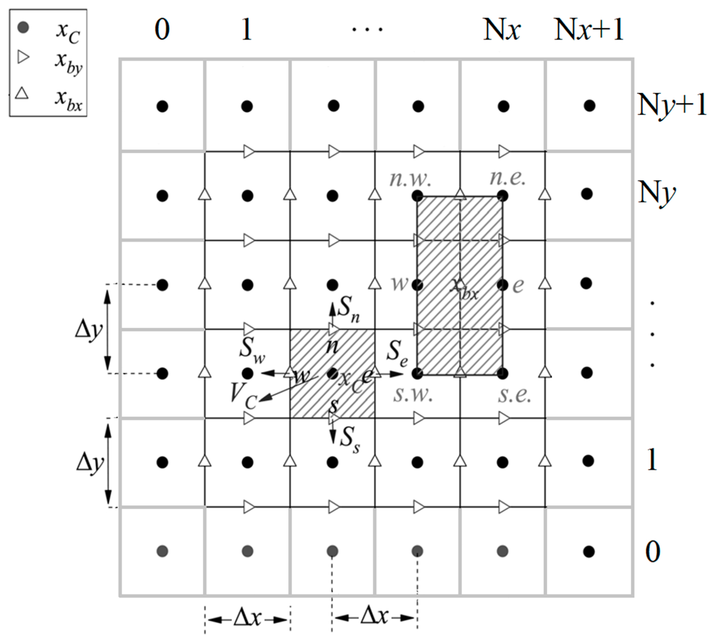
2. Numerical Method
2.1. Simplified Governing Equations of DUGKS with Force Term
2.2. Three Methods for Calculating Interface Flux
2.2.1. Original DUGKS
2.2.2. Optimize DUGKS
2.2.3. Simpson–DUGKS
2.3. Comparative Analysis
3. Numerical Test
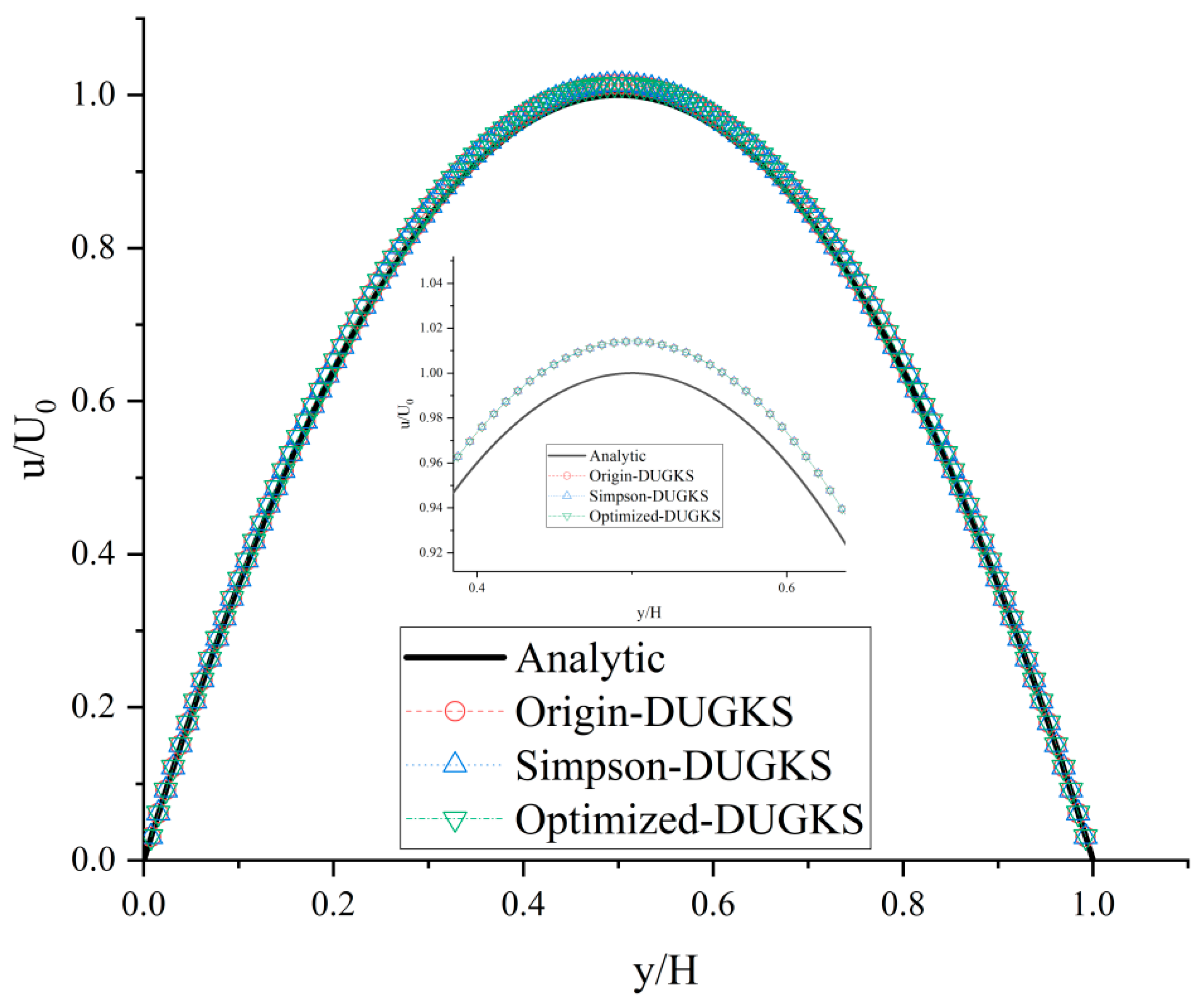
3.1. Couette Flow
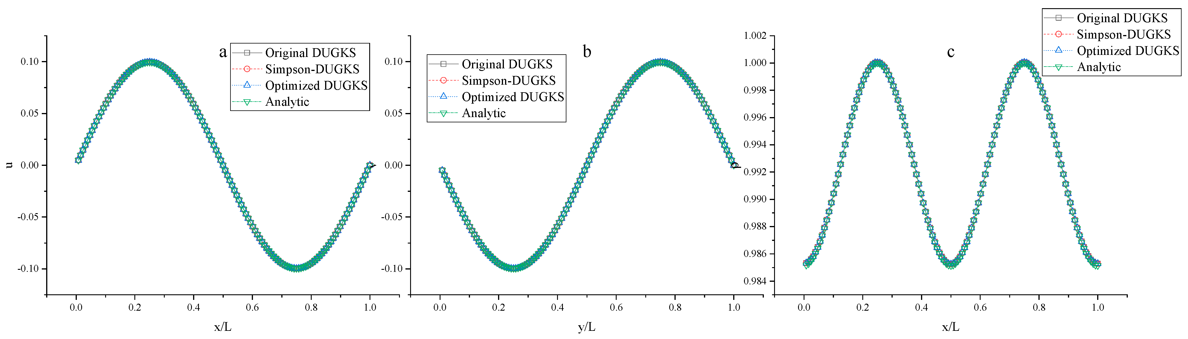
3.2. Poiseuille Flow
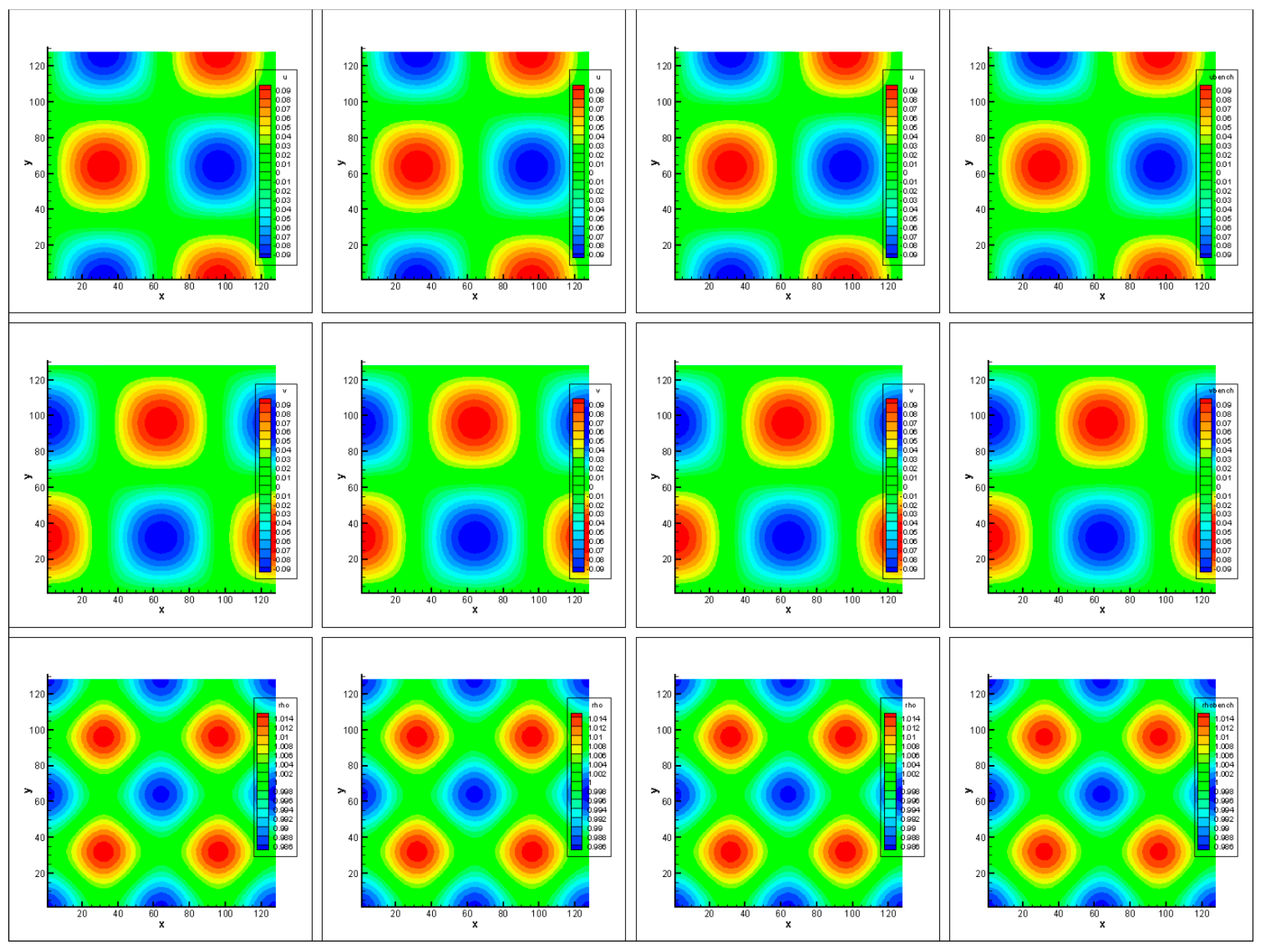
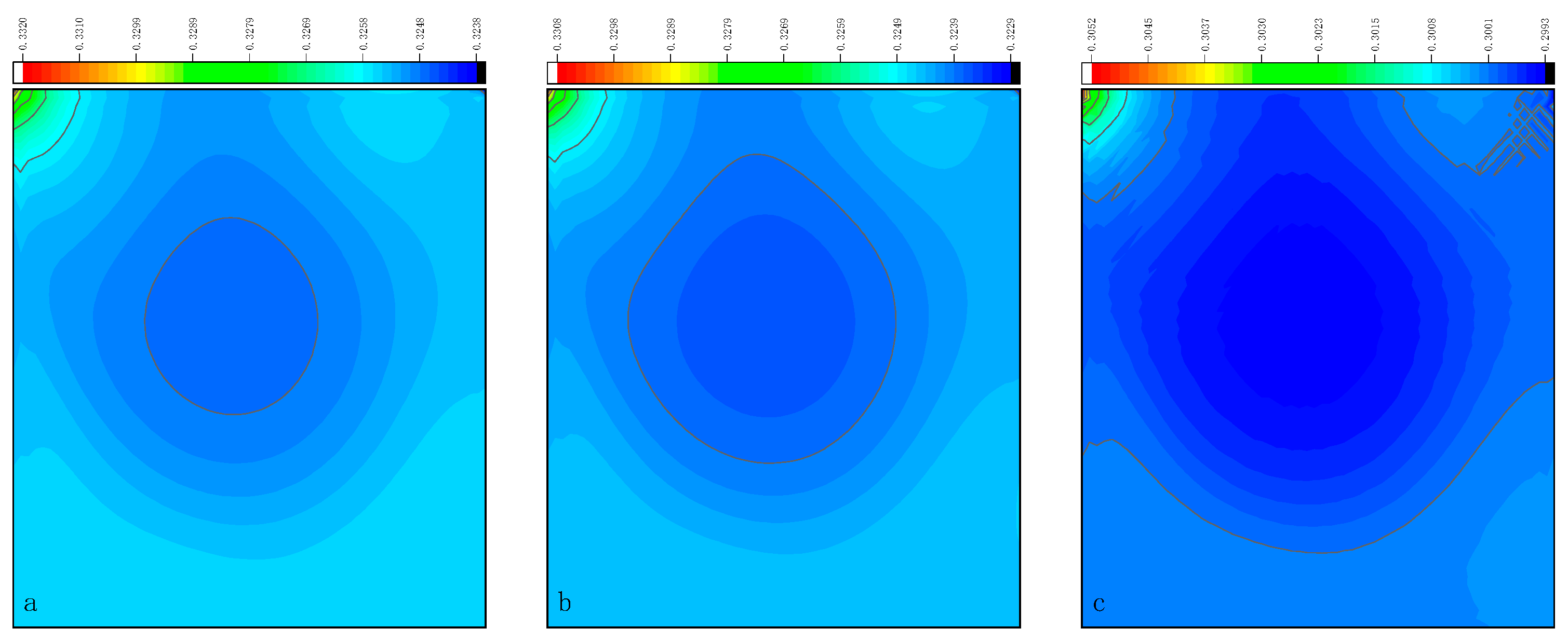
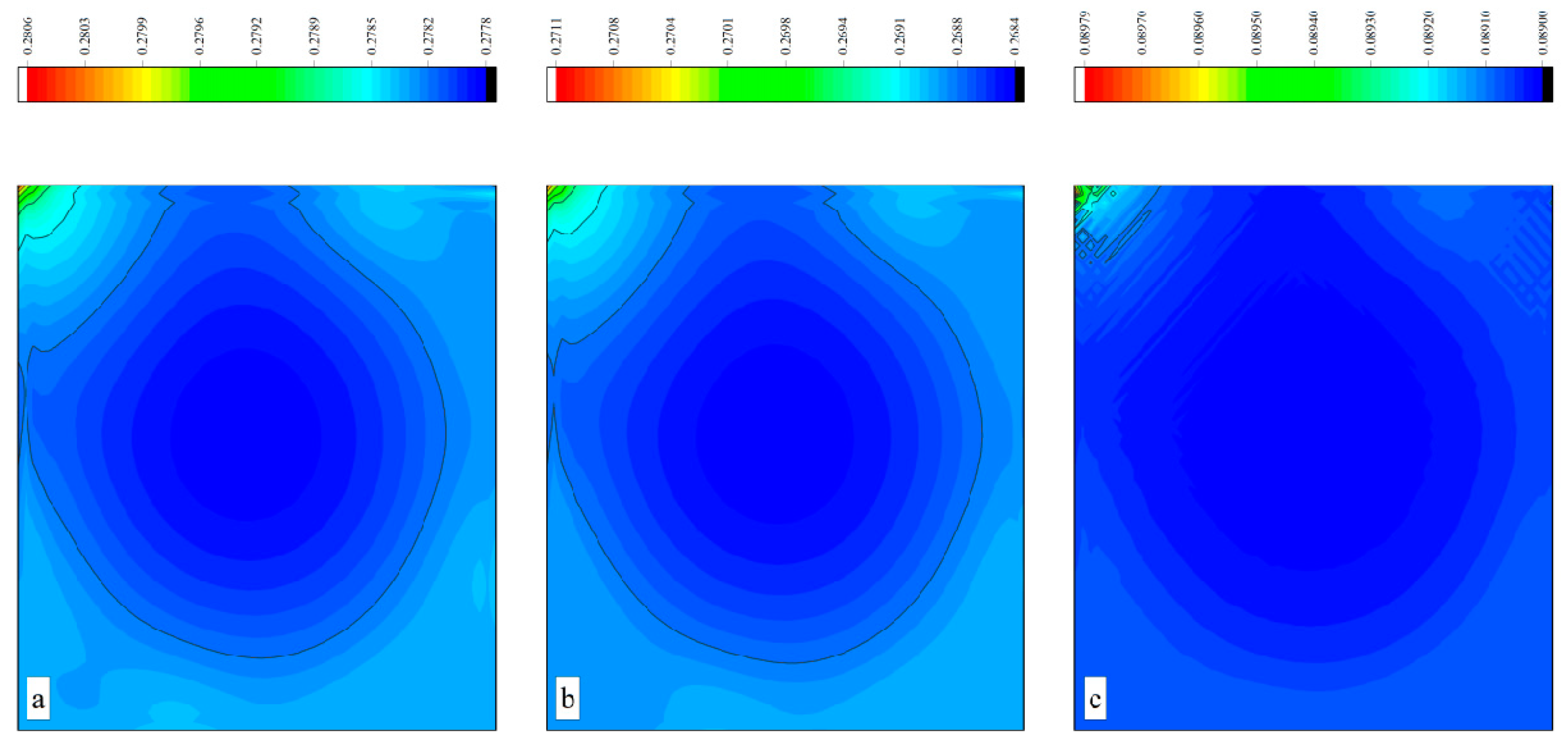
3.3. Taylor–Green Vortex Flow
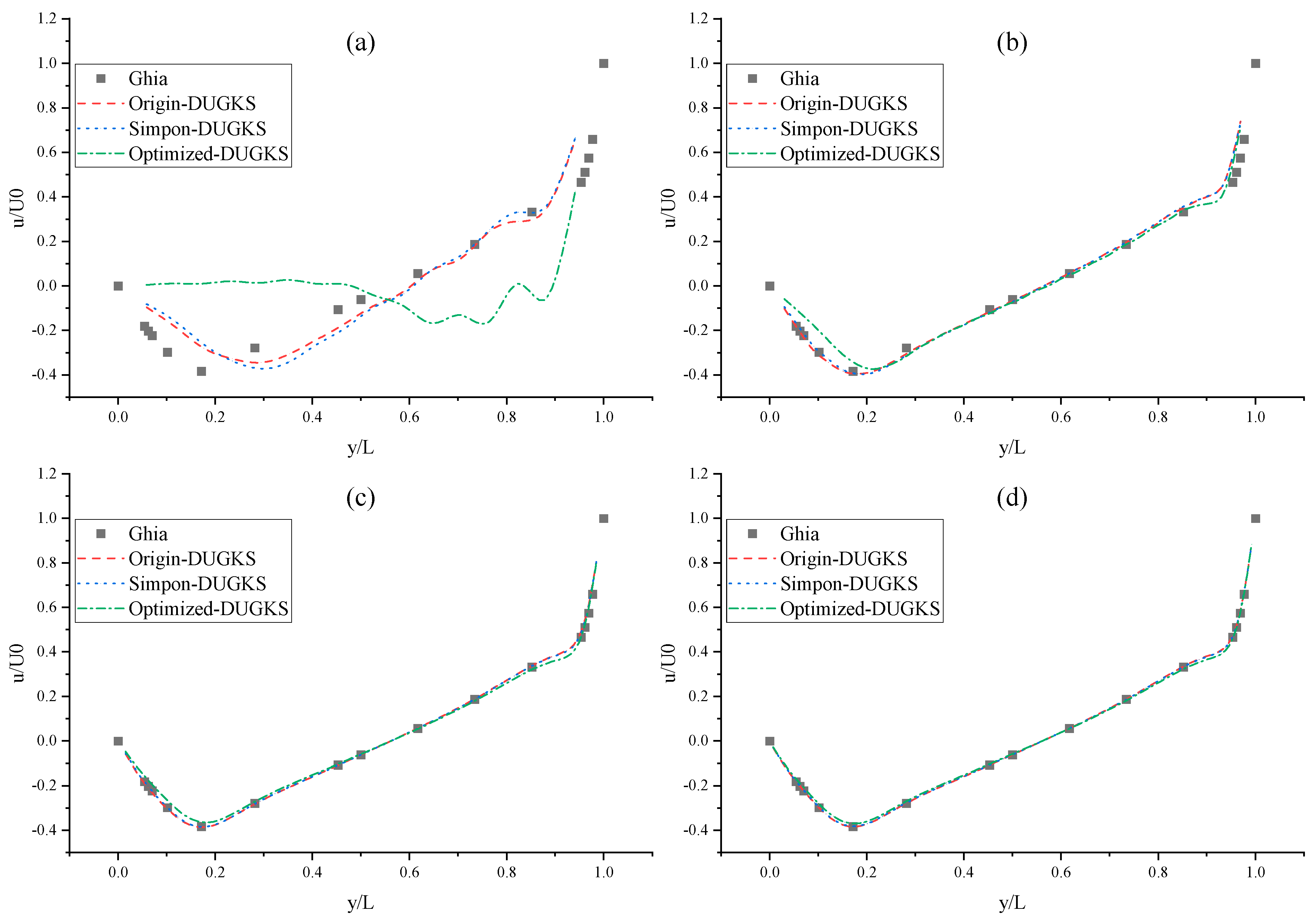
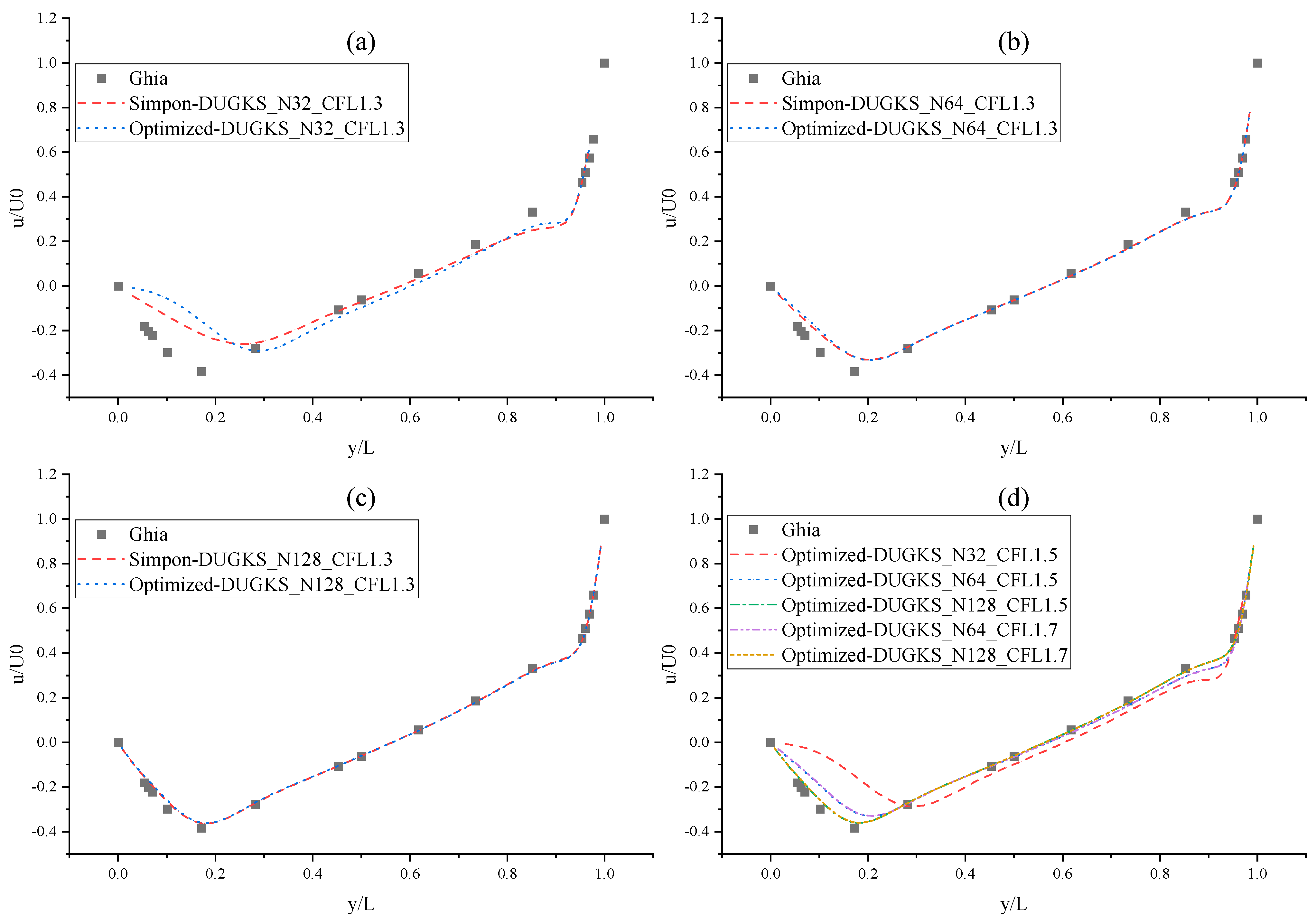
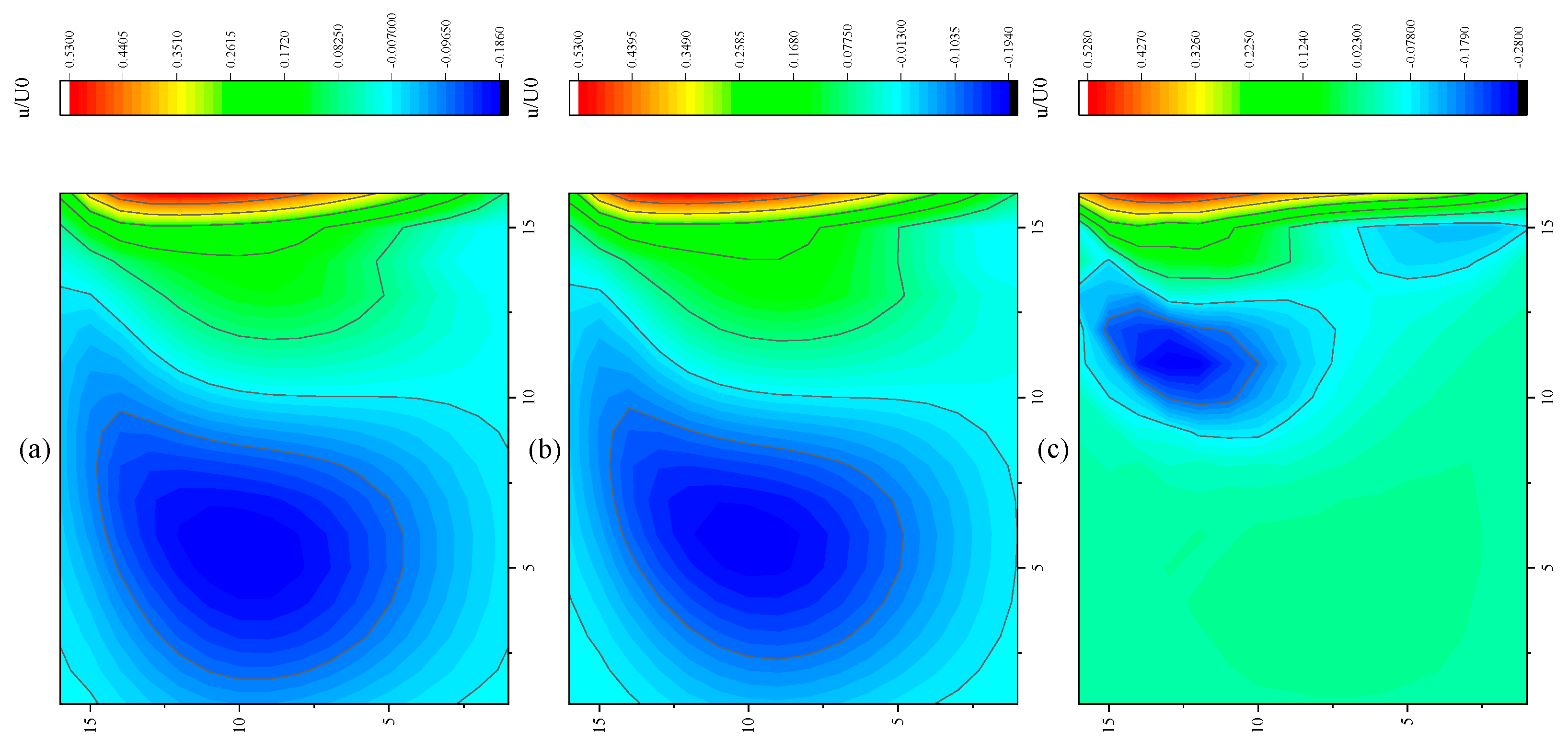
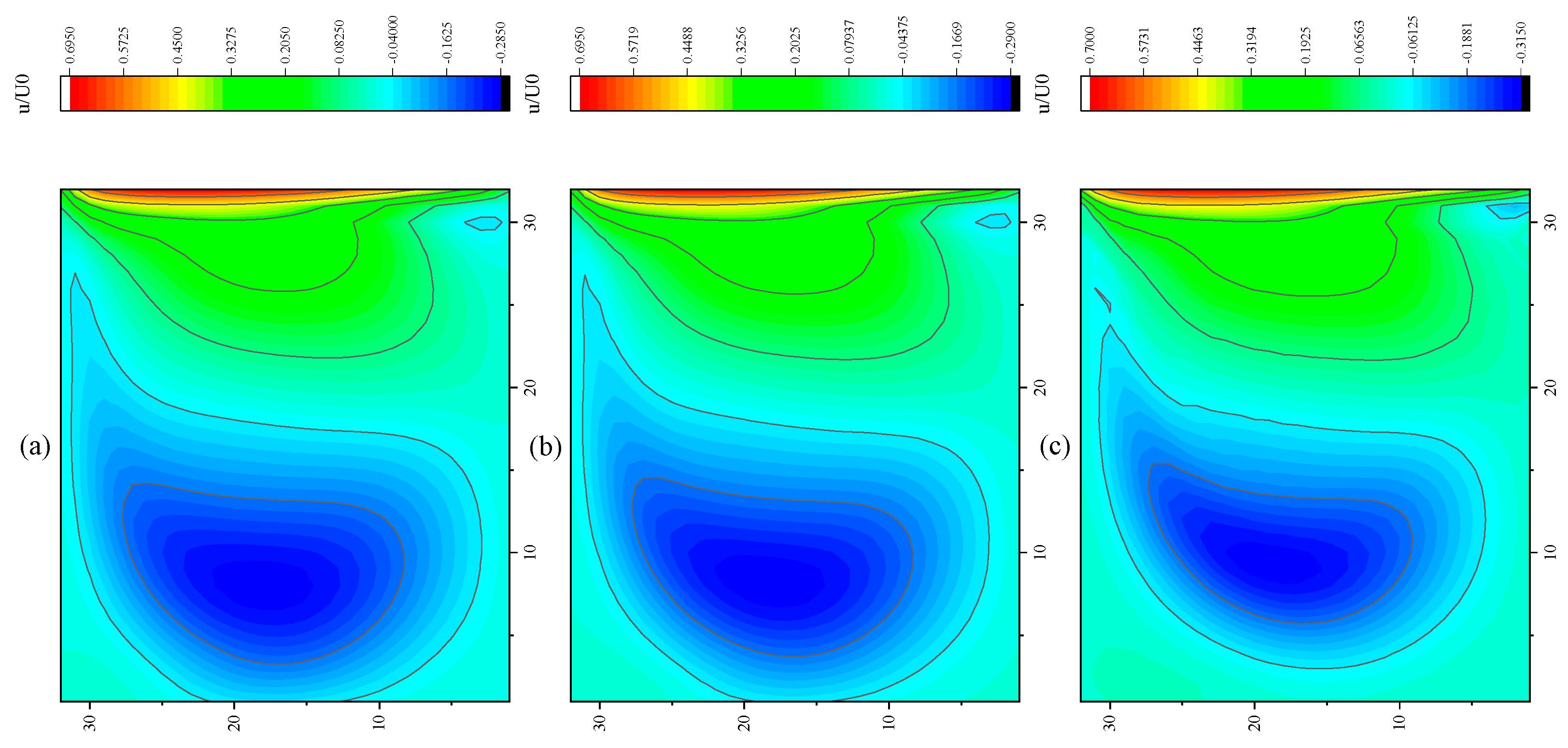
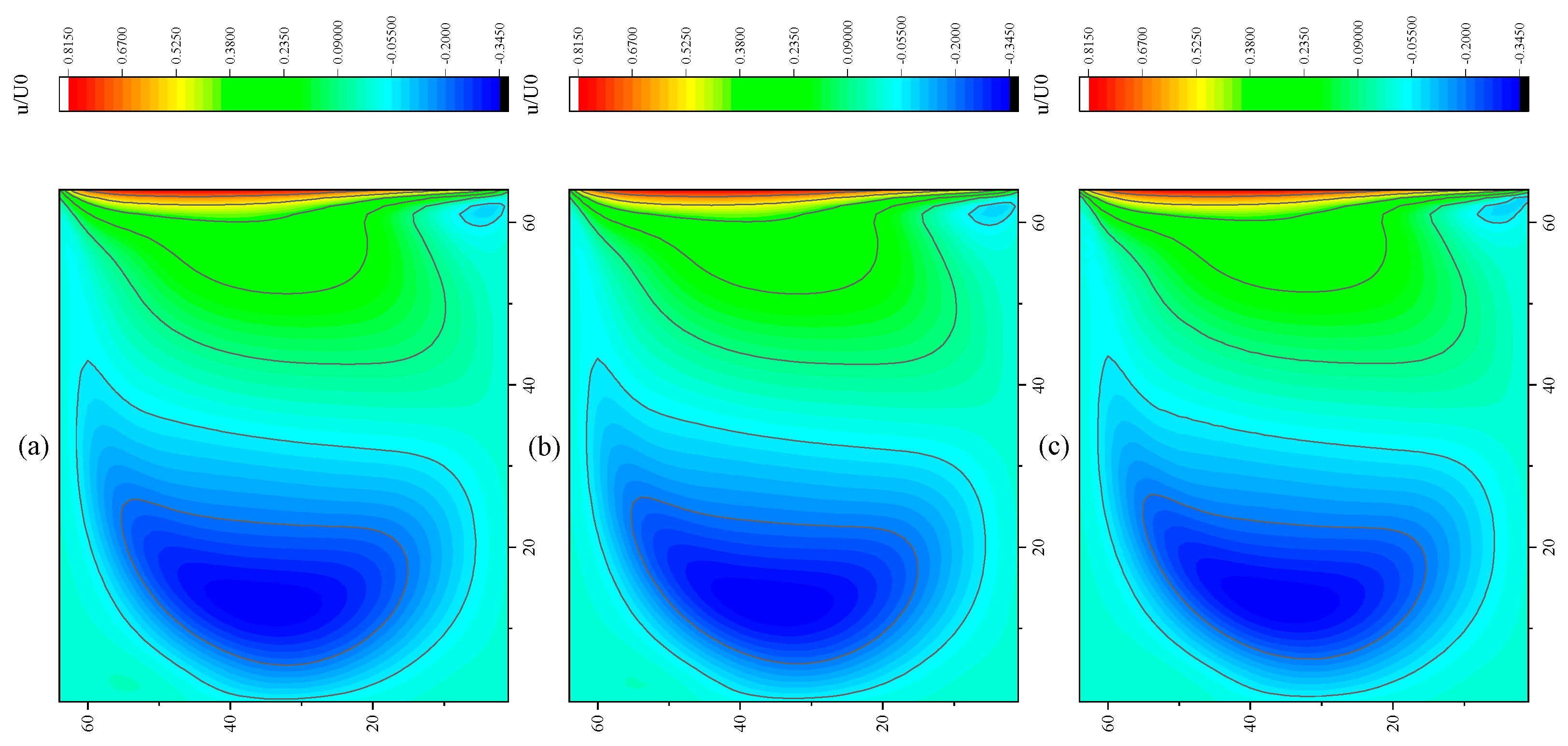
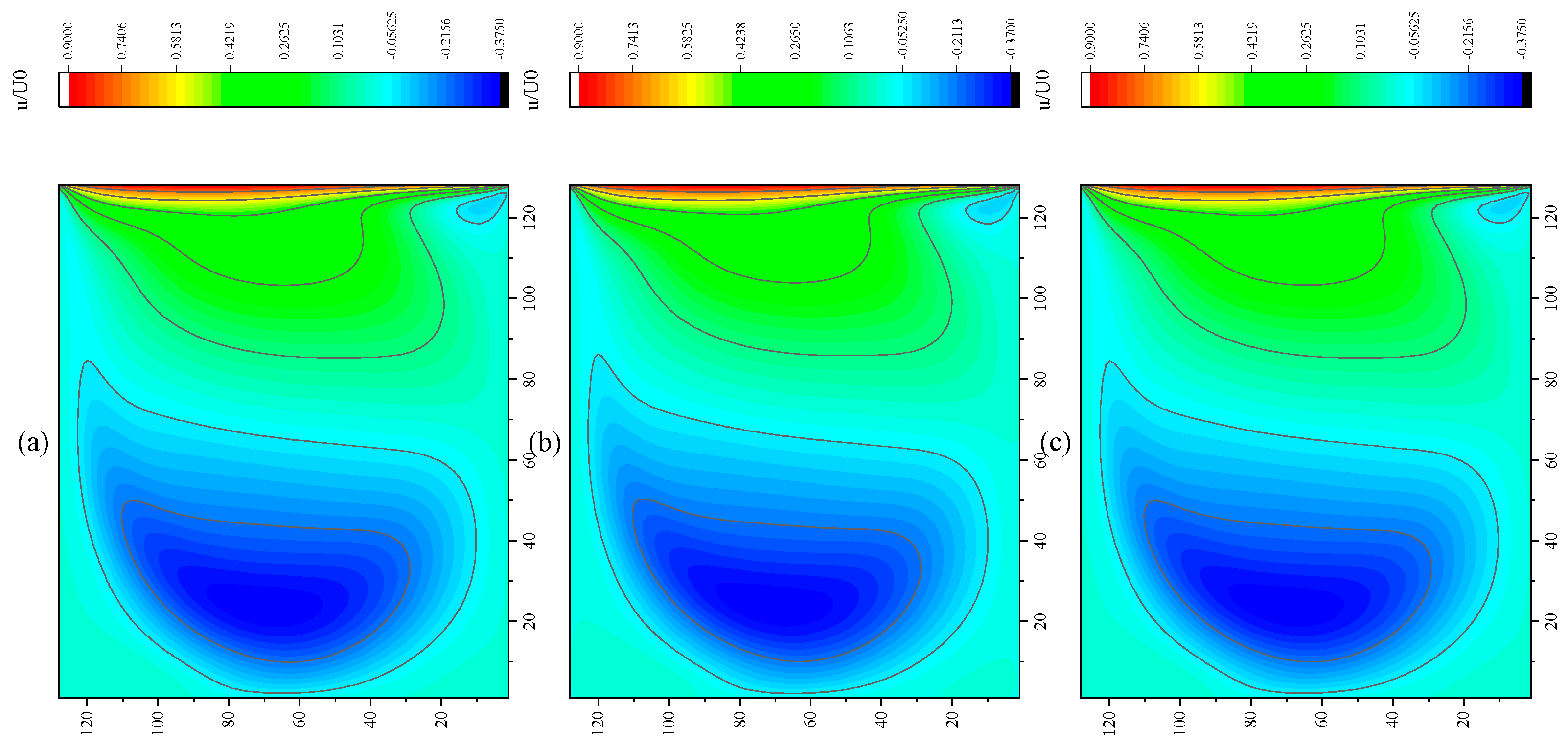
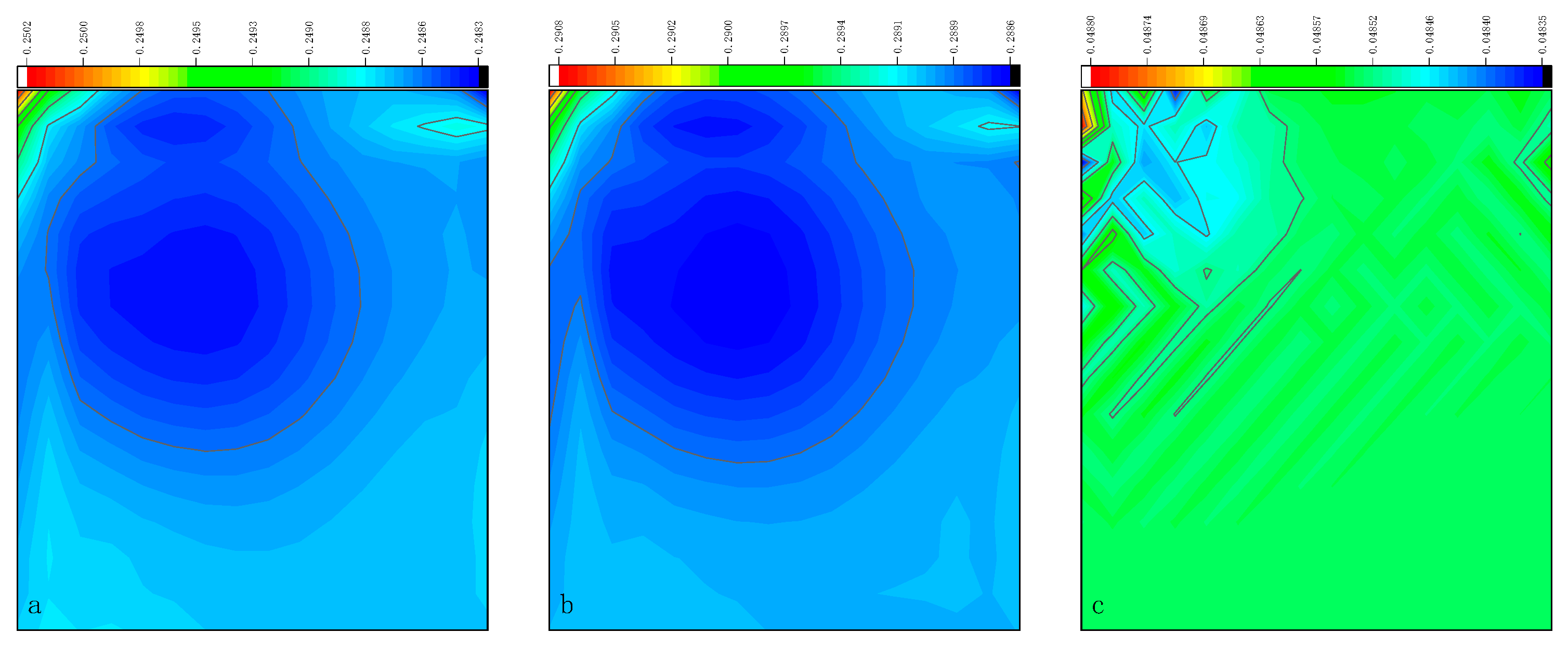
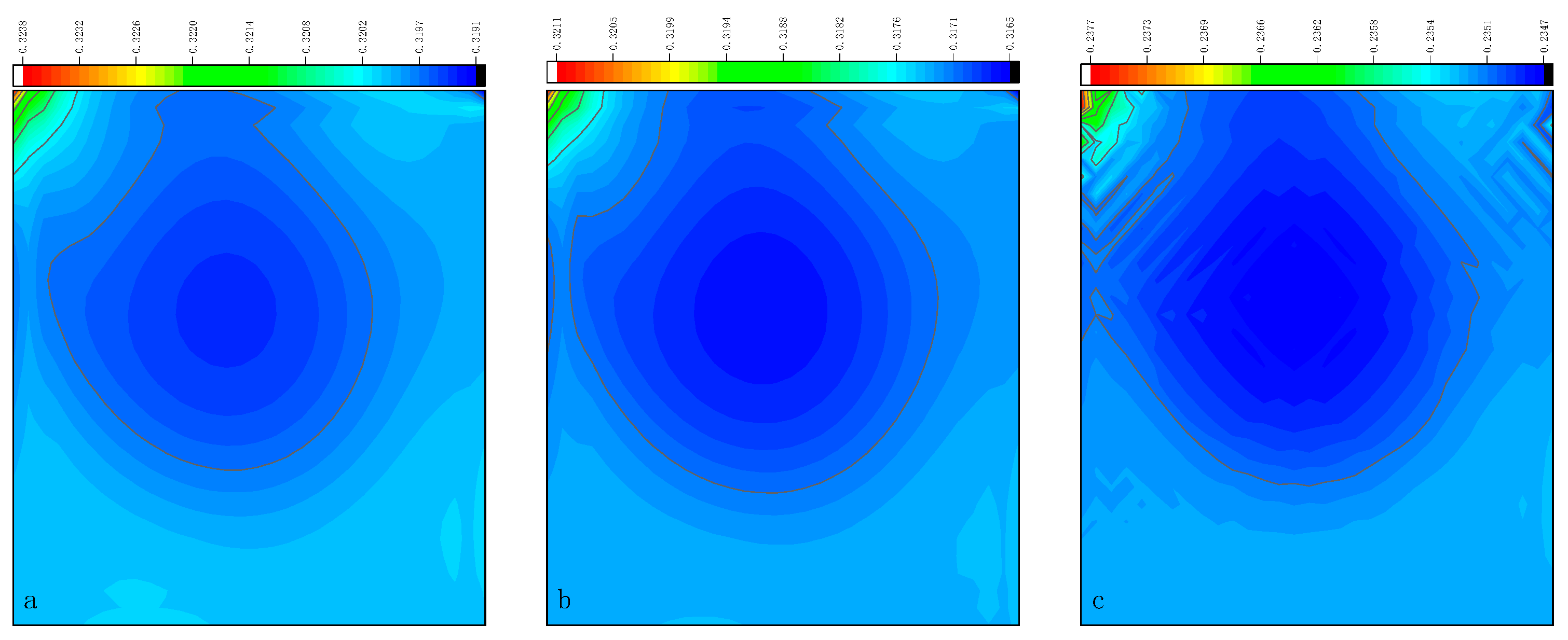
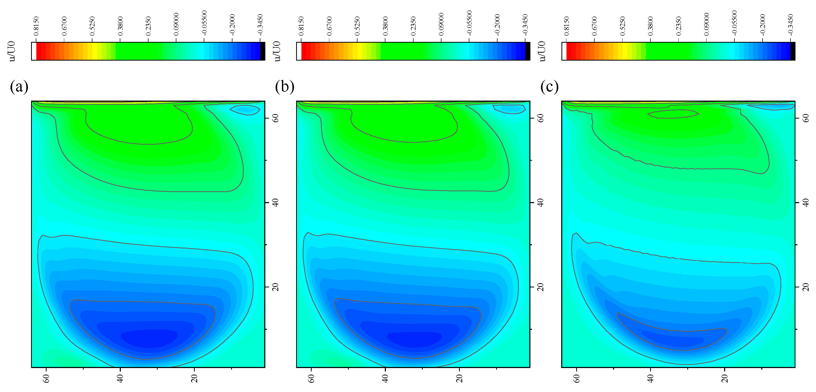
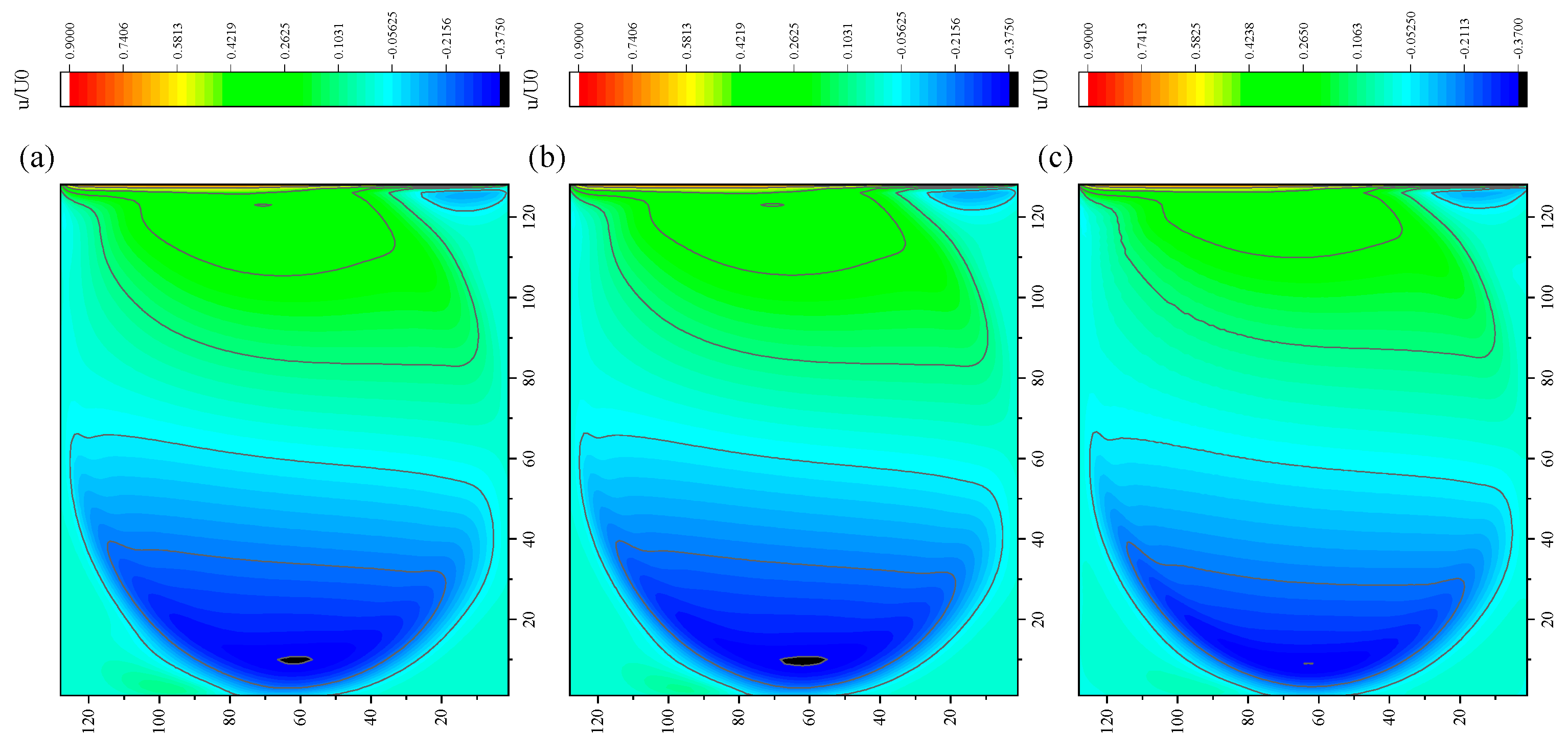
3.4. Lid-Driven Cavity Flow
- (1)
- Spatial and temporal truncation errors: optimized DUGKS can introduce truncation errors, which may accumulate and lead to significant density errors in specific flow regimes, especially when the flow has complex structures or high gradients.
- (2)
- Dispersion and dissipation errors: Optimized DUGKS can suffer from dispersion and dissipation errors. In some flows, these errors might be amplified, causing the density waves to propagate at incorrect speeds or with distorted shapes. This can lead to a discrepancy between the numerical solution and the exact solution, manifesting as a large density error.
- (3)
- Complex flow structures: flow with complex structures, such as those involving multiple vortices, can pose challenges for optimized DUGKS. The method might have difficulties in accurately resolving these intricate structures, leading to errors in the density field. For example, in a flow with contact discontinuities, the optimized DUGKS may not capture the sharp density gradients at the discontinuities, resulting in a smeared density profile and larger errors.
4. Conclusions
- (1)
- In the numerical test of Taylor–Green vortex flow, the stability of the three methods is consistent under different grid numbers. Compared with the analytical solution of velocity, the L2 error of optimized DUGKS is the smallest under the same number of grids, but the L2 error of optimized DUGKS is the largest under the same number of grids compared with the analytical solution of density. In terms of computational efficiency, among the three methods, optimized DUGKS has the least computational time, while Simpson–DUGKS has the most computational time.
- (2)
- In the numerical test of the lid-driven cavity flow, the calculation time of the optimized DUGKS can be reduced by about 77% at most, compared with the original DUGKS. It should be noted that, when CFL = 0.1 and N = 16, the calculation time of optimized DUGKS increases by about 40% compared with the original DUGKS. When CFL = 0.95 and N = 16, the calculation time of Simpson–DUGKS is reduced by about 59% compared with the original DUGKS. In terms of stability, the optimized DUGKS can still be computationally stable at large CFL numbers (CFL = 1.5 and 1.7). In terms of accuracy, the results of optimized DUGKS deviate more from the reference results, especially in the case of a small grid number. For example, when CFL = 0.95 and N = 16, the error of horizontal velocity contours obtained by optimized DUGKS is obviously large. This may be explained by the fact that the optimized DUGKS requires the fewest number of auxiliary points.
Funding
Institutional Review Board Statement
Data Availability Statement
Conflicts of Interest
Appendix A
References
- Guo, Z.; Xu, K. Progress of discrete unified gas-kinetic scheme for multiscale flows. Adv. Aerodyn. 2021, 3, 6. [Google Scholar] [CrossRef]
- Tian, B.; Li, L.; Meng, Y.; Huang, B. Multiscale modeling of different cavitating flow patterns around NACA66 hydrofoil. Phys. Fluids 2022, 34, 103322. [Google Scholar] [CrossRef]
- Pfeiffer, M. A part-based ellipsoidal statistical Bhatnagar-Gross-Krook solution with variable weights for the simulation of large density gradients in micro-and nano-nozzles. Phys. Fluids 2020, 32, 112009. [Google Scholar] [CrossRef]
- Yang, L.; Shu, C.; Yang, W.; Wu, J. An improved three-dimensional implicit discovery velocity method on unstructured meshes for all Knudsen number flows. J. Comput. Phys. 2019, 396, 738–760. [Google Scholar] [CrossRef]
- Liu, Z.J.; Shu, C.; Chen, S.Y.; Liu, W.; Yuan, Z.Y.; Yang, L.M. Development of explicit formulations of G45-based gas kinetic scheme for simulation of continuum and rarefied flows. Phys. Rev. E 2022, 105, 045302. [Google Scholar] [CrossRef]
- Wang, Y.; Zhong, C.; Liu, S. Arbitrary Lagrangian-Eulerian-type discrete unified gas kinetic scheme for low-speed continuum and rarefied flow simulations with moving boundaries. Phys. Rev. E 2019, 100, 063310. [Google Scholar] [CrossRef]
- Li, Z.-H.; Hu, W.-Q.; Wu, J.-L.; Peng, A.-P. Improved gas-kinetic unified algorithm for high rarefied to continuum flows by computable modeling of the Boltzmann equation. Phys. Fluids 2021, 33, 126114. [Google Scholar] [CrossRef]
- Liu, S.; Zhong, C.; Fang, M. Simplified unified wave-particle method with quantified model-competition mechanism for numerical calculation of multiscale flows. Phys. Rev. E 2020, 102, 013304. [Google Scholar] [CrossRef] [PubMed]
- Wang, Y.; Liu, S.; Zhuo, C.S.; Zhong, C. A discrete unified gas kinetic scheme for solving fluid-structure interaction problems in low-speed continuum and rarefied flows. Acta Aerodyn. Sin. 2022, 40, 87–97. [Google Scholar]
- Li, S.Y.; Zhang, C.; Tan, S. Gas-kinetic scheme and its applications in re-entry flows. Acta Aerodyn. Sin. 2018, 36, 885–890. [Google Scholar]
- Yang, L.; Li, Z.; Shu, C. Advances on discrete velocity method and its application in all Knudsen number flows. J. Nanjing Univ. Aeronaut. Astronaut. 2022, 54, 537–551. [Google Scholar]
- Votta, R.; Schettino, A.; Bonfiglioli, A. Hypersonic high altitude aerothermodynamics of a space re-entry vehicle. Aerosp. Sci. Technol. 2013, 25, 253–265. [Google Scholar] [CrossRef]
- Bird, G.A. Molecular Gas Dynamics and the Direct Simulation of Gas Flows; Oxford University Press: London, UK, 1994. [Google Scholar]
- Jing, F. Rarefied Gas Dynamics: Advances and Applications. Adv. Mech. 2013, 43, 185–201. [Google Scholar]
- Fang, M.; Li, Z.; Li, Z.; Li, C. DSMC approach for rarefied air ionization during space reentry. Commun. Comput. Phys. 2018, 23, 1167–1190. [Google Scholar]
- Li, Z.H.; Zhang, H.X. Gas-kinetic numerical studies of three-dimensional complex flows on spacecraft re-entry. J. Comput. Phys. 2009, 228, 1116–1138. [Google Scholar] [CrossRef]
- Xu, K.; Huang, J.C. A unified gas kinetic scheme for continuum and rarefied flows. J. Comput. Phys. 2010, 229, 7747–7764. [Google Scholar] [CrossRef]
- Guo, Z.; Xu, K.; Wang, R. Discrete unified gas kinetic scheme for all Knudsen number flows: Low-speed isothermal case. Phys. Rev. E 2013, 88, 033305. [Google Scholar] [CrossRef]
- Liu, C.; Zhu, Y.; Xu, K. Unified gas-kinetic wave-particle methods I: Continuum and rarefied gas flow. J. Comput.-Tional Phys. 2020, 40, 108977. [Google Scholar] [CrossRef]
- Fan, G.; Zhao, W.; Jiang, Z.; Chen, W. Study of Shock Structures Using the Unified Gas-Kinetic Wave-Particle Method with Various BGK Models. Int. J. Comput. Fluid Dyn. 2022, 36, 44–62. [Google Scholar] [CrossRef]
- Fan, G.; Zhao, W.; Yao, S.; Jiang, Z.; Chen, W. The implementation of the three-dimensional unified gas-kinetic wave-particle method on multiple graphics processing units. Phys. Fluids 2023, 35, 086108. [Google Scholar] [CrossRef]
- Wang, P.; Zhu, L.; Guo, Z.; Xu, K. A Comparative Study of LBE and DUGKS Methods for Nearly Incompressible Flows. Commun. Comput. Phys. 2015, 17, 657–681. [Google Scholar] [CrossRef]
- Wu, C.; Shi, B.; Chai, Z.; Wang, P. Discrete Unified Gas Kinetic Scheme with a Force Term for Incompressible Fluid Flows. Comput. Math. Appl. 2016, 71, 2608–2629. [Google Scholar] [CrossRef]
- Guo, Z.; Wang, R.; Xu, K. Discrete Unified Gas Kinetic Scheme for all Knudsen Number Flows. II. Thermal Compressible Case. Phys. Rev. E 2015, 91, 033313. [Google Scholar] [CrossRef] [PubMed]
- Wang, P.; Wang, L.-P.; Guo, Z. Comparison of the lattice Boltzmann equation and discrete unified gas-kinetic scheme methods for direct numerical simulation of decaying turbulent flows. Phys. Rev. E 2016, 94, 043304. [Google Scholar] [CrossRef]
- Bo, Y.; Wang, P.; Guo, Z.; Wang, L.-P. DUGKS simulations of three-dimensional Taylor–Green vortex flow and turbulent channel flow. Comput. Fluids 2017, 155, 9–21. [Google Scholar] [CrossRef]
- Wang, L.P.; Huq, P.; Guo, Z. Simulations of turbulence and dispersion in idealized urban canopies using a new kinetic scheme. In Proceedings of the 68th Annual Meeting of the APS Division of Fluid Dynamics, Boston, MA, USA, 22–24 November 2015. [Google Scholar]
- Wen, X.; Wang, L.-P.; Guo, Z.; Zhakebayev, D.B. Laminar to turbulent flow transition inside the boundary layer adjacent to isothermal wall of natural convection flow in a cubical cavity. Int. J. Heat Mass Transf. 2021, 167, 120822. [Google Scholar] [CrossRef]
- Zhu, L.; Guo, Z. Numerical study of nonequilibrium gas flow in a microchannel with a ratchet surface. Phys. Rev. E 2017, 95, 023113. [Google Scholar] [CrossRef]
- Zhu, L.; Yang, X.; Guo, Z. Thermally induced rarefied gas flow in a three-dimensional enclosure with square cross-section. Phys. Rev. Fluids 2017, 2, 123402. [Google Scholar] [CrossRef]
- Wang, P.; Ho, M.T.; Wu, L.; Guo, Z.; Zhang, Y. A comparative study of discrete velocity methods for low-speed rarefied gas flows. Comput. Fluids 2018, 161, 33–46. [Google Scholar] [CrossRef]
- Zhu, L.; Guo, Z. Application of discrete unified gas kinetic scheme to thermally induced nonequilibrium flows. Comput. Fluids 2019, 193, 103613. [Google Scholar] [CrossRef]
- Wang, Y.; Liu, S.; Zhuo, C.; Zhong, C. Investigation of nonlinear squeeze-film damping involving rarefied gas effect in micro-electro-mechanical systems. Comput. Math. Appl. 2022, 114, 188–209. [Google Scholar] [CrossRef]
- Wang, L.P.; Guo, Z.; Wang, J. Improving the discrete unified gas kinetic scheme for efficient simulation of three-dimensional compressible turbulence. In Proceedings of the 71st Annual Meeting of the APS Division of Fluid Dynamics, Atlanta, GA, USA, 18–20 November 2018. [Google Scholar]
- Chen, T.; Wen, X.; Wang, L.-P.; Guo, Z.; Wang, J.; Chen, S. Simulation of three-dimensional compressible decaying isotropic turbulence using a redesigned discrete unified gas kinetic scheme. Phys. Fluids 2020, 32, 125104. [Google Scholar] [CrossRef]
- Wen, X.; Wang, L.-P.; Guo, Z. Designing a consistent implementation of the discrete unified gas-kinetic scheme for the simulation of three-dimensional compressible natural convection. Phys. Fluids 2021, 33, 046101. [Google Scholar] [CrossRef]
- Chen, T.; Wen, X.; Wang, L.-P.; Guo, Z.; Wang, J.; Chen, S.; Zhakebayev, D.B. Simulation of three-dimensional forced compressible isotropic turbulence by a redesigned discrete unified gas kinetic scheme. Phys. Fluids 2022, 34, 025106. [Google Scholar] [CrossRef]
- Zhang, C.; Yang, K.; Guo, Z. A discrete unified gas-kinetic scheme for immiscible two-phase flows. Int. J. Heat Mass Transf. 2018, 126, 1326–1336. [Google Scholar] [CrossRef]
- Yang, Z.; Zhong, C.; Zhuo, C. Phase-field method based on discrete unified gas-kinetic scheme for large-density-ratio two-phase flows. Phys. Rev. E 2019, 99, 043302. [Google Scholar] [CrossRef]
- Zhang, C.; Liang, H.; Guo, Z.; Wang, L.-P. Discrete unified gas-kinetic scheme for the conservative Allen-Cahn equation. Phys. Rev. E 2022, 105, 045317. [Google Scholar] [CrossRef]
- Tao, S.; Zhang, H.; Guo, Z.; Wang, L.-P. A combined immersed boundary and discrete unified gas kinetic scheme for particle–fluid flows. J. Comput. Phys. 2018, 375, 498–518. [Google Scholar] [CrossRef]
- Tao, S.; Chen, B.; Yang, X.; Huang, S. Second-order accurate immersed boundary-discrete unified gas kinetic scheme for fluid-particle flows. Comput. Fluids 2018, 165, 54–63. [Google Scholar] [CrossRef]
- Tao, S.; He, Q.; Wang, L.; Chen, B.; Chen, J.; Lin, Y. Discrete unified gas kinetic scheme simulation of conjugate heat transfer problems in complex geometries by a ghost-cell interface method. Appl. Math. Comput. 2021, 404, 126228. [Google Scholar] [CrossRef]
- He, Q.; Tao, S.; Yang, X.; Lu, W.; He, Z. Discrete unified gas kinetic scheme simulation of microflows with complex geometries in Cartesian grid. Phys. Fluids 2021, 33, 042005. [Google Scholar] [CrossRef]
- Zhang, Y.; Zhu, L.; Wang, R.; Guo, Z. Discrete unified gas kinetic scheme for all Knudsen number flows. III. Binary gas mixtures of Maxwell molecules. Phys. Rev. E 2018, 97, 053306. [Google Scholar] [CrossRef] [PubMed]
- Zhang, Y.; Zhu, L.; Wang, P.; Guo, Z. Discrete unified gas kinetic scheme for flows of binary gas mixture based on the McCormack model. Phys. Fluids 2019, 31, 017101. [Google Scholar] [CrossRef]
- Tao, S.; Wang, L.; Ge, Y.; He, Q. Application of half-way approach to discrete unified gas kinetic scheme for simulating pore-scale porous media flows. Comput. Fluids 2021, 214, 104776. [Google Scholar] [CrossRef]
- Liu, P.; Wang, P.; Jv, L.; Guo, Z. A Coupled Discrete Unified Gas-Kinetic Scheme for Convection Heat Transfer in Porous Media. Commun. Comput. Phys. 2021, 29, 265–291. [Google Scholar] [CrossRef]
- Gu, Q.; Ho, M.-T.; Zhang, Y. Computational methods for pore-scale simulation of rarefied gas flow. Comput. Fluids 2021, 222, 104932. [Google Scholar] [CrossRef]
- Liu, H.; Quan, L.; Chen, Q.; Zhou, S.; Cao, Y. Discrete unified gas kinetic scheme for electrostatic plasma and its comparison with the particle-in-cell method. Phys. Rev. E 2020, 101, 043307. [Google Scholar] [CrossRef]
- Liu, H.; Shi, F.; Wan, J.; He, X.; Cao, Y. Discrete unified gas kinetic scheme for a reformulated BGK–Vlasov–Poisson system in all electrostatic plasma regimes. Comput. Phys. Commun. 2020, 255, 107400. [Google Scholar] [CrossRef]
- Guo, Z.; Xu, K. Discrete unified gas kinetic scheme for multiscale heat transfer based on the phonon Boltzmann transport equation. Int. J. Heat Mass Transf. 2016, 102, 944–958. [Google Scholar] [CrossRef]
- Zhang, C.; Guo, Z. Discrete unified gas kinetic scheme for multiscale heat transfer with arbitrary temperature difference. Int. J. Heat Mass Transf. 2019, 134, 1127–1136. [Google Scholar] [CrossRef]
- Luo, X.-P.; Yi, H.-L. A discrete unified gas kinetic scheme for phonon Boltzmann transport equation accounting for phonon dispersion and polarization. Int. J. Heat Mass Transf. 2017, 114, 970–980. [Google Scholar] [CrossRef]
- Luo, X.-P.; Wang, C.-H.; Zhang, Y.; Yi, H.-L.; Tan, H.-P. Multiscale solutions of radiative heat transfer by the discrete unified gas kinetic scheme. Phys. Rev. E 2018, 97, 063302. [Google Scholar] [CrossRef] [PubMed]
- Song, X.; Zhang, C.; Zhou, X.; Guo, Z. Discrete unified gas kinetic scheme for multiscale anisotropic radiative heat transfer. Adv. Aerodyn. 2020, 2, 3. [Google Scholar] [CrossRef]
- Wang, L.; Liang, H.; Xu, J.-R. Optimized discrete unified gas kinetic scheme for continuum and rarefied flows. Phys. Fluids 2023, 35, 017106. [Google Scholar] [CrossRef]
- Zhu, L.; Wang, P.; Guo, Z. Performance evaluation of the general characteristics based off-lattice Boltzmann scheme and DUGKS for low speed continuum flows. J. Comput. Phys. 2017, 333, 227–246. [Google Scholar] [CrossRef]
- Ghia, U.; Ghia, K.; Shin, C. High-Re solutions for incompressible flow using the Navier-Stokes equations and a multigrid method. J. Comput. Phys. 1982, 48, 387–411. [Google Scholar] [CrossRef]
- Luo, L.-S.; Liao, W.; Chen, X.; Peng, Y.; Zhang, W. Numerics of the lattice Boltzmann method: Effects of collision models on the lattice Boltzmann simulations. Phys. Rev. E 2011, 83, 056710. [Google Scholar] [CrossRef]


| CFL | Nx = Ny | L2 Error | Number of Steps | CPU Time (s) | ||||
|---|---|---|---|---|---|---|---|---|
| Original DUGKS | Simpson– DUGKS | Optimized DUGKS | Δ1 | Δ2 | ||||
| 0.1 | 16 | 2.38 × 10⁻⁵ | 270,000 | 63.91 | 111.81 | 49.18 | 74.95% | 23.05% |
| 32 | 4.55 × 10⁻⁵ | 477,000 | 462.34 | 817.19 | 322.38 | 76.75% | 30.27% | |
| 64 | 9.02 × 10⁻⁵ | 859,000 | 3818.79 | 6515.43 | 2408.6 | 70.62% | 36.93% | |
| 128 | 1.78 × 10⁻⁴ | 1,563,000 | 26,650.16 | 35,060.65 | 21,806.14 | 31.56% | 18.18% | |
| 0.5 | 16 | 3.81 × 10⁻⁶ | 63,000 | 17.12 | 29.45 | 12.02 | 72.02% | 29.79% |
| 32 | 8.16 × 10⁻⁶ | 112,000 | 111.58 | 211.32 | 78.73 | 89.39% | 29.44% | |
| 64 | 1.73 × 10⁻⁵ | 203,000 | 919.18 | 1871.22 | 541.88 | 103.57% | 41.05% | |
| 128 | 3.52 × 10⁻⁵ | 373,000 | 8172.24 | 10,395.84 | 4409.96 | 27.21% | 46.04% | |
| 0.95 | 16 | 1.90 × 10⁻⁶ | 35,000 | 11.32 | 18.09 | 6.43 | 59.81% | 43.20% |
| 32 | 3.68 × 10⁻⁶ | 63,000 | 72.59 | 122.96 | 44.57 | 69.39% | 38.60% | |
| 64 | 8.41 × 10⁻⁶ | 114,000 | 529.62 | 1090.94 | 303.46 | 105.99% | 42.70% | |
| 128 | 1.75 × 10⁻⁵ | 210,000 | 4107.69 | 6703.03 | 2447.27 | 63.18% | 40.42% | |
| 1 | 16 | 1.42 × 10⁻⁶ | 34,000 | 11.16 | 16.49 | 6.66 | 47.76% | 40.32% |
| 32 | 3.56 × 10⁻⁶ | 60,000 | 75.02 | 113.61 | 43.75 | 51.44% | 41.68% | |
| 64 | 7.81 × 10⁻⁶ | 109,000 | 499.07 | 1098.91 | 334.94 | 120.19% | 32.89% | |
| 128 | 1.71 × 10⁻⁵ | 200,000 | 3943.93 | 6306.43 | 2365.88 | 59.90% | 40.01% | |
| 1.5 | 16 | 1.18 × 10⁻⁶ | 23,000 | 6.96 | 12.36 | 5.18 | 77.59% | 25.57% |
| 32 | 2.61 × 10⁻⁶ | 41,000 | 48.11 | 82.77 | 33.65 | 72.04% | 30.06% | |
| 64 | 5.38 × 10⁻⁶ | 75,000 | 383.26 | 802.2 | 239.67 | 109.31% | 37.47% | |
| 128 | 1.08 × 10⁻⁵ | 139,000 | 2849.27 | 4691.96 | 1679.31 | 64.67% | 41.06% | |
| 1.7 | 16 | - | - | - | - | - | - | - |
| 32 | 7.44 × 10⁻⁷ | 21,000 | 6.32 | 12.37 | 3.85 | 95.73% | 39.08% | |
| 64 | 1.96 × 10⁻⁶ | 37,000 | 46.24 | 79.87 | 25.35 | 72.73% | 45.18% | |
| 128 | 4.64 × 10⁻⁶ | 67,000 | 342.42 | 698.74 | 180.01 | 104.06% | 47.43% | |
| CFL | L2 Error | Number of Steps | CPU Time (s) | ||||
|---|---|---|---|---|---|---|---|
| Original DUGKS | Simpson– DUGKS | Optimized DUGKS | Δ1 | Δ2 | |||
| 0.95 | 1.878066 × 10⁻³ | 11,831,000 | 270,194.67 | 278,382.72 | 165,471.65 | 3.03% | 38.76% |
| 1.5 | 1.189824 × 10⁻³ | 8,060,000 | 199,466.71 | 202,131.9 | 172,020.05 | 1.32% | 13.76% |
| 1.7 | 1.049839 × 10⁻³ | 7,249,000 | 188,147.77 | 233,224.22 | 158,852.38 | 23.96% | 15.57% |
| CFL | Nx = Ny | CPU Time (s) | L2 Error | Number of Steps | ||||
|---|---|---|---|---|---|---|---|---|
| Original DUGKS | Simpson– DUGKS | Optimized DUGKS | Δ1 | Δ2 | ||||
| 0.1 | 16 | 100.79 | 149.77 | 75.44 | 48.60% | 25.15% | 0.102804 | 274,000 |
| 32 | 720.16 | 1169.49 | 499.15 | 62.39% | 30.69% | 0.058279 | 485,000 | |
| 64 | 5426.69 | 7813.4 | 3637.99 | 43.98% | 32.96% | 0.030417 | 877,000 | |
| 128 | 37,932.5 | 51,146.37 | 28,019.24 | 34.84% | 26.13% | 0.015342 | 1,598,000 | |
| 0.5 | 16 | 23.7 | 33.49 | 17.63 | 41.31% | 25.61% | 0.095353 | 64,000 |
| 32 | 161.33 | 223.71 | 116.22 | 38.67% | 27.96% | 0.056502 | 113,000 | |
| 64 | 1324.72 | 1976.8 | 840.31 | 49.22% | 36.57% | 0.030133 | 207,000 | |
| 128 | 9188.03 | 13,185.13 | 6398.8 | 43.50% | 30.36% | 0.015423 | 380,000 | |
| 0.95 | 16 | 12.93 | 20.25 | 9.91 | 56.61% | 23.36% | 0.096755 | 36,000 |
| 32 | 87.2 | 124.37 | 65.94 | 42.63% | 24.38% | 0.056514 | 63,000 | |
| 64 | 661.76 | 1018.5 | 469.13 | 53.91% | 29.11% | 0.030074 | 116,000 | |
| 128 | 5390.39 | 7759.16 | 3656.11 | 43.94% | 32.17% | 0.015404 | 213,000 | |
| 1 | 16 | 13.37 | 19.98 | 10.69 | 49.44% | 20.04% | 0.097037 | 34,000 |
| 32 | 93.56 | 142.11 | 72.68 | 51.89% | 22.32% | 0.056554 | 61,000 | |
| 64 | 734.11 | 1155.93 | 489.51 | 57.46% | 33.32% | 0.030076 | 110,000 | |
| 128 | 5205.93 | 7473.29 | 3441.71 | 43.55% | 33.89% | 0.015403 | 204,000 | |
| 1.5 | 16 | 10.03 | 15.51 | 7.04 | 54.64% | 29.81% | 0.100341 | 24,000 |
| 32 | 68.14 | 109.34 | 44.25 | 60.46% | 35.06% | 0.057129 | 42,000 | |
| 64 | 522.65 | 829.57 | 319.33 | 58.72% | 38.90% | 0.030144 | 76,000 | |
| 128 | 3630.2 | 5254.6 | 2467.22 | 44.75% | 32.04% | 0.015396 | 141,000 | |
| 1.7 | 16 | 9.64 | 14.83 | 5.97 | 53.84% | 38.07% | 0.101791 | 21,000 |
| 32 | 66.03 | 103.21 | 41.76 | 56.31% | 36.76% | 0.057416 | 38,000 | |
| 64 | 464.12 | 730.12 | 303.73 | 57.31% | 34.56% | 0.030189 | 68,000 | |
| 128 | - | - | - | - | - | - | - | |
| CPU Time (s) | L2 Error | Number of Steps | ||||
|---|---|---|---|---|---|---|
| Original DUGKS | Simpson–DUGKS | Optimized DUGKS | Δ1 | Δ2 | ||
| 249,234.44 | 255,189.79 | 138,468.52 | 2.39% | 44.44% | 0.01405448 | 7,455,000 |
| Nx = Ny | Convergence Error | L2 Error of Horizontal Velocity | L2 Error of Vertical Velocity | L2 Error of Density |
|---|---|---|---|---|
| 16 | 3.796248 × 10⁻³ | 1.407493 × 10⁻¹ | 1.390931 × 10⁻¹ | 1.753841 × 10⁻⁵ |
| 32 | 9.123970 × 10⁻⁴ | 3.110016 × 10⁻³ | 3.103787 × 10⁻³ | 1.435340 × 10⁻⁶ |
| 64 | 2.206357 × 10⁻⁴ | 6.720014 × 10⁻⁵ | 6.717489 × 10⁻⁵ | 1.309586 × 10⁻⁷ |
| 128 | 5.624876 × 10⁻⁵ | 2.920428 × 10⁻⁶ | 2.920423 × 10⁻⁶ | 1.276418 × 10⁻⁸ |
| Nx = Ny | Convergence Error | L2 Error of Horizontal Velocity | L2 Error of Vertical Velocity | L2 Error of Density |
|---|---|---|---|---|
| 16 | 4.106844 × 10⁻³ | 1.309639 × 10⁻¹ | 1.308380 × 10⁻¹ | 1.860117 × 10⁻⁵ |
| 32 | 9.011641 × 10⁻⁴ | 2.687649 × 10⁻³ | 2.684068 × 10⁻³ | 1.275103 × 10⁻⁶ |
| 64 | 2.099531 × 10⁻⁴ | 6.469734 × 10⁻⁵ | 6.463202 × 10⁻⁵ | 1.285961 × 10⁻⁷ |
| 128 | 5.535000 × 10⁻⁵ | 2.830797 × 10⁻⁶ | 2.830400 × 10⁻⁶ | 1.319192 × 10⁻⁸ |
| Nx = Ny | Convergence Error | L2 Error of Horizontal Velocity | L2 Error of Vertical Velocity | L2 Error of Density |
|---|---|---|---|---|
| 16 | 1.216599 × 10⁻³ | 6.491338 × 10⁻² | 5.887564 × 10⁻² | 5.567707 × 10⁻⁵ |
| 32 | 3.288855 × 10⁻⁴ | 1.800740 × 10⁻³ | 1.774188 × 10⁻³ | 3.178361 × 10⁻⁶ |
| 64 | 1.920442 × 10⁻⁴ | 6.009158 × 10⁻⁵ | 5.993777 × 10⁻⁵ | 1.746339 × 10⁻⁷ |
| 128 | 5.446530 × 10⁻⁵ | 2.732364 × 10⁻⁶ | 2.731590 × 10⁻⁶ | 1.393446 × 10⁻⁸ |
| Nx = Ny | Original DUGKS | Simpson–DUGKS | Optimized DUGKS | Δ1 | Δ2 |
|---|---|---|---|---|---|
| 16 | 4.89 | 5.96 | 4.32 | 22% | 12% |
| 32 | 13.68 | 17.58 | 11.03 | 29% | 19% |
| 64 | 47.45 | 61.52 | 37.01 | 30% | 22% |
| 128 | 183.57 | 236.9 | 138.77 | 29% | 24% |
| CFL | Nx = Ny | Original DUGKS | Simpson–DUGKS | Optimized DUGKS | Δ1 | Δ2 |
|---|---|---|---|---|---|---|
| 0.1 | 16 | 46.48 | 102.26 | 65.1 | 120% | −40% |
| 32 | 512.08 | 907.5 | 334.52 | 77% | 35% | |
| 64 | 3836.81 | 8557.54 | 2664.58 | 123% | 31% | |
| 128 | 31,612.86 | 82,837.44 | 23,141.43 | 162% | 27% | |
| 0.95 | 16 | 67.17 | 27.73 | 16.61 | −59% | 75% |
| 32 | 62.41 | 84.73 | 55.25 | 36% | 11% | |
| 64 | 454.8 | 591.63 | 308.51 | 30% | 32% | |
| 128 | 3184.97 | 4371.63 | 2128.85 | 37% | 33% | |
| 1.3 | 16 | - | - | - | / | / |
| 32 | - | 80.09 | 67.03 | / | / | |
| 64 | - | 574.24 | 417.9 | / | / | |
| 128 | - | 4629.64 | 2677.79 | / | / | |
| 1.5 | 16 | - | - | - | / | / |
| 32 | - | - | 41.02 | / | / | |
| 64 | - | - | 218.79 | / | / | |
| 128 | - | - | 1241.96 | / | / | |
| 1.7 | 16 | - | - | - | / | / |
| 32 | - | - | - | / | / | |
| 64 | - | - | 196.97 | / | / | |
| 128 | - | - | 1090.08 | / | / |
| CFL | N | Original DUGKS | Simpson–DUGKS | Optimized DUGKS | Δ1 | Δ2 |
|---|---|---|---|---|---|---|
| 0.1 | 32 | 3503.67 | 7056.31 | cannot converge | 101% | / |
| 64 | 32,251.44 | 49,593.47 | 19513.29 | 54% | 39% | |
| 128 | 239,206.58 | 440,938.26 | 206,700.12 | 84% | 14% | |
| 0.95 | 64 | 5997.67 | 7347.21 | 2963.74 | 23% | 51% |
| 128 | 74,691.44 | 52,091.25 | 33,552.44 | −30% | 55% |
Disclaimer/Publisher’s Note: The statements, opinions and data contained in all publications are solely those of the individual author(s) and contributor(s) and not of MDPI and/or the editor(s). MDPI and/or the editor(s) disclaim responsibility for any injury to people or property resulting from any ideas, methods, instructions or products referred to in the content. |
© 2025 by the author. Licensee MDPI, Basel, Switzerland. This article is an open access article distributed under the terms and conditions of the Creative Commons Attribution (CC BY) license (https://creativecommons.org/licenses/by/4.0/).
Share and Cite
Guo, W. Comparative Study on Flux Solution Methods of Discrete Unified Gas Kinetic Scheme. Entropy 2025, 27, 528. https://doi.org/10.3390/e27050528
Guo W. Comparative Study on Flux Solution Methods of Discrete Unified Gas Kinetic Scheme. Entropy. 2025; 27(5):528. https://doi.org/10.3390/e27050528
Chicago/Turabian StyleGuo, Wenqiang. 2025. "Comparative Study on Flux Solution Methods of Discrete Unified Gas Kinetic Scheme" Entropy 27, no. 5: 528. https://doi.org/10.3390/e27050528
APA StyleGuo, W. (2025). Comparative Study on Flux Solution Methods of Discrete Unified Gas Kinetic Scheme. Entropy, 27(5), 528. https://doi.org/10.3390/e27050528