
Alternating Direction Method of Multipliers-Based Constant Modulus Waveform Design for Dual-Function Radar-Communication Systems

 , , , and
Abstract
1. Introduction
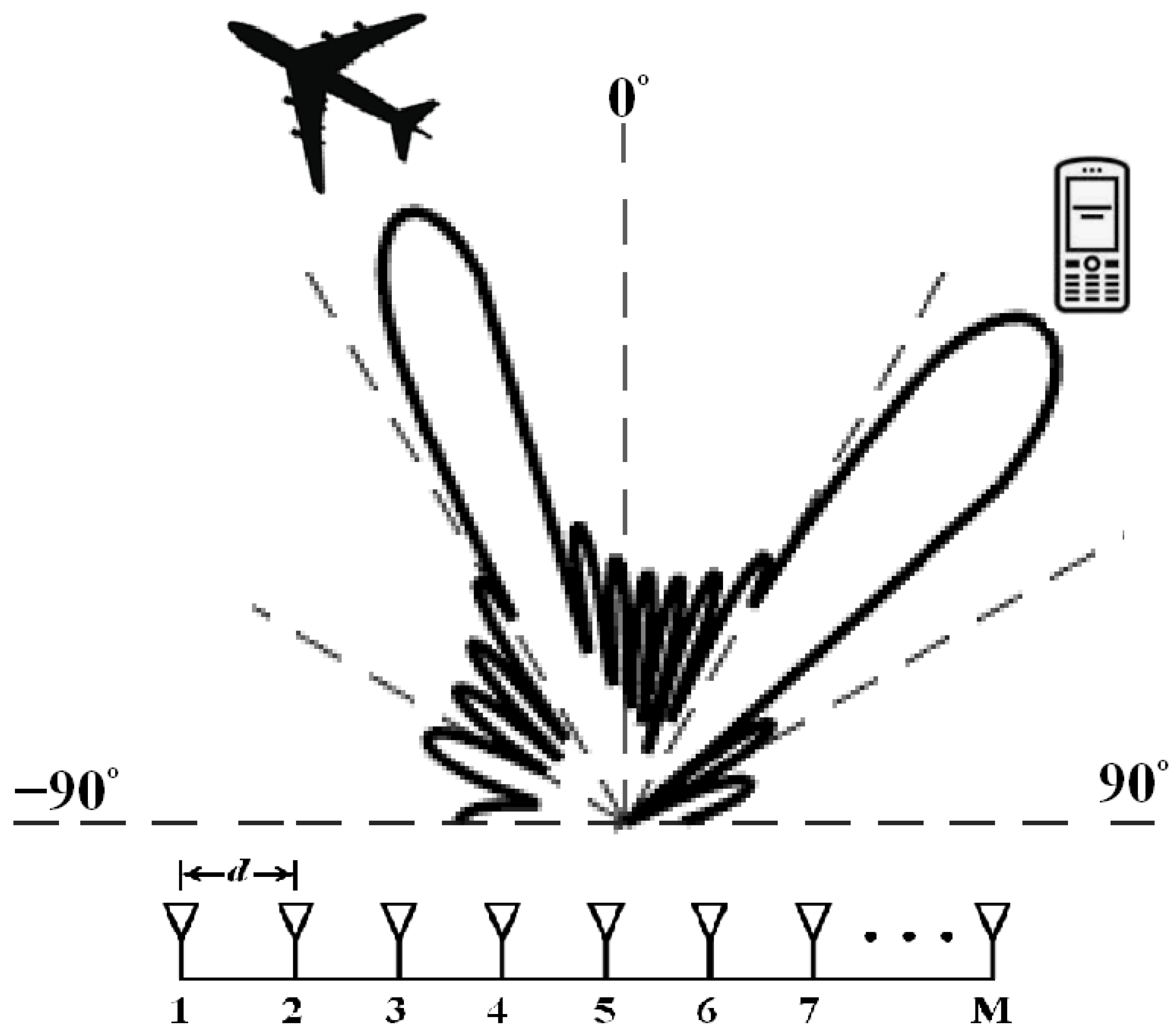
2. Signal Model
3. Problem Formulation
3.1. Vectorization
3.2. Realization
4. ADMM Formulation and Solution
4.1. Update of
4.2. Update of
4.3. Termination Criteria of the Algorithm
| Algorithm 1: Summary of the proposed algorithm |
Input: Step (1) Initialize: and , , , , . Step (2) While the termination criteria, Equation (34), are not satisfied, do Step (3) Update using Equation (25) Step (4) Update using Equation (29) Step (5) Update using Equation (23c) Step (6) Update using Equation (23d) Step (7) Update using Equation (23e) Step (8) Step (9) End while Output: |
4.4. Penalty Parameter Selection
5. Simulation Results and Analysis
5.1. Computational Complexity Analysis
5.2. Data Rate Performance
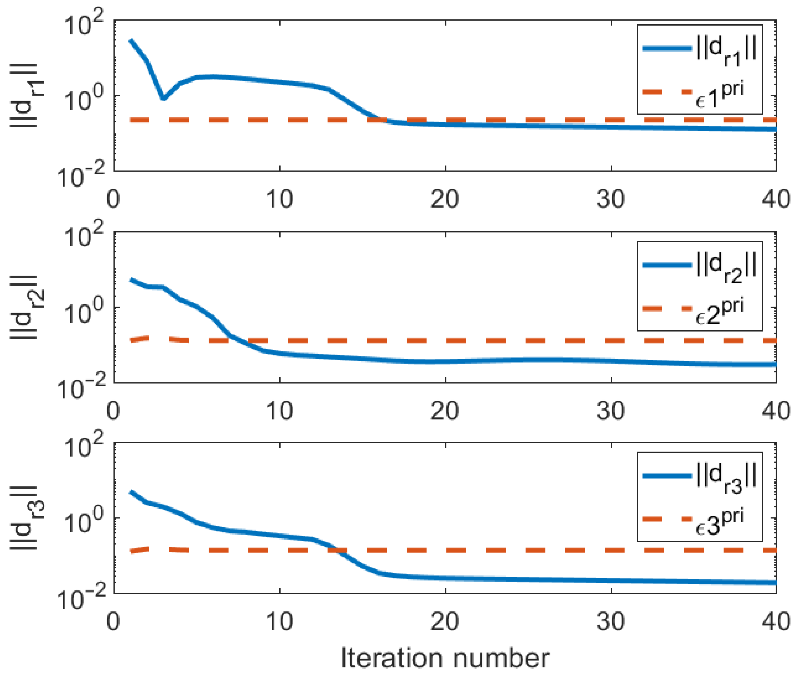
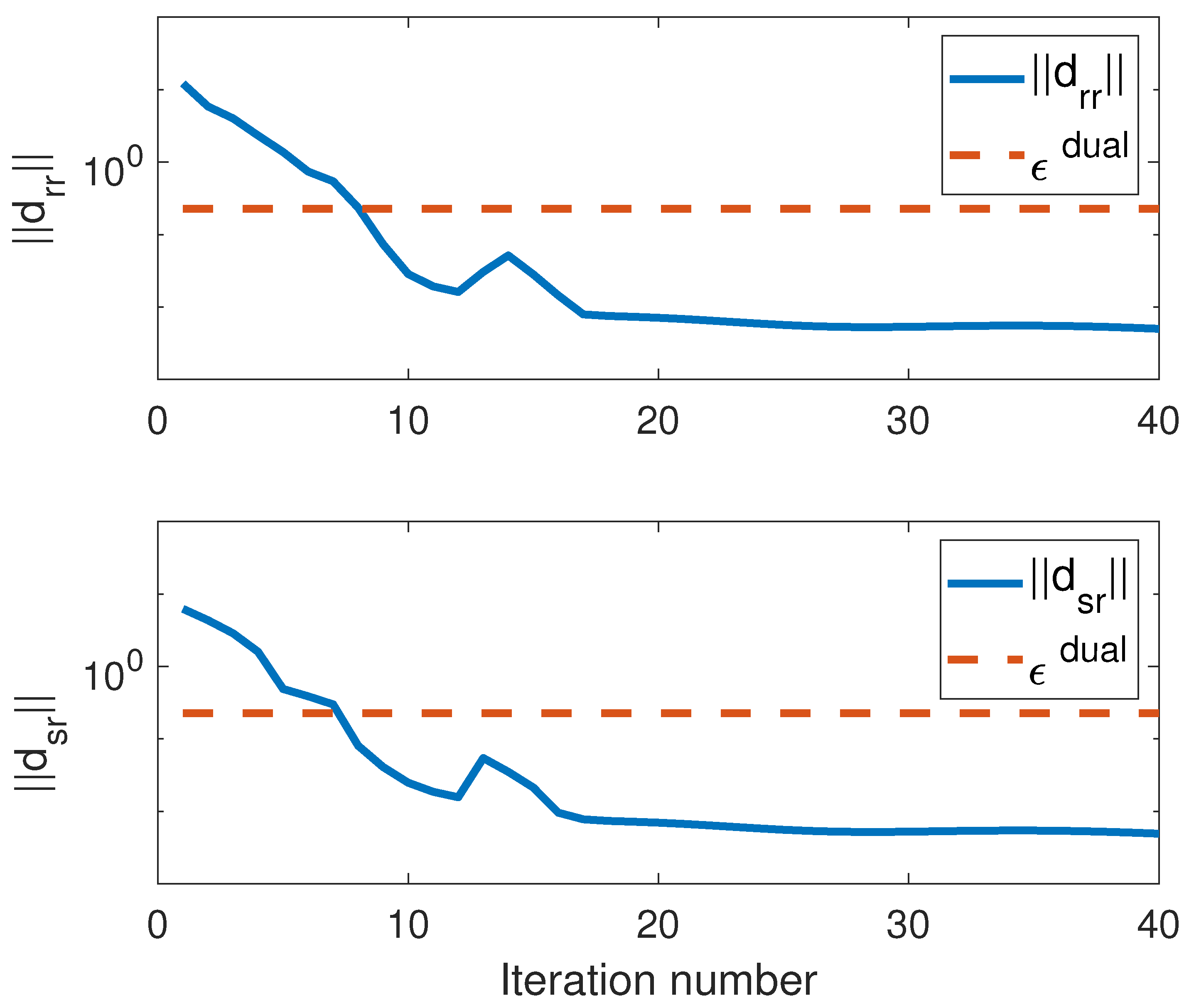
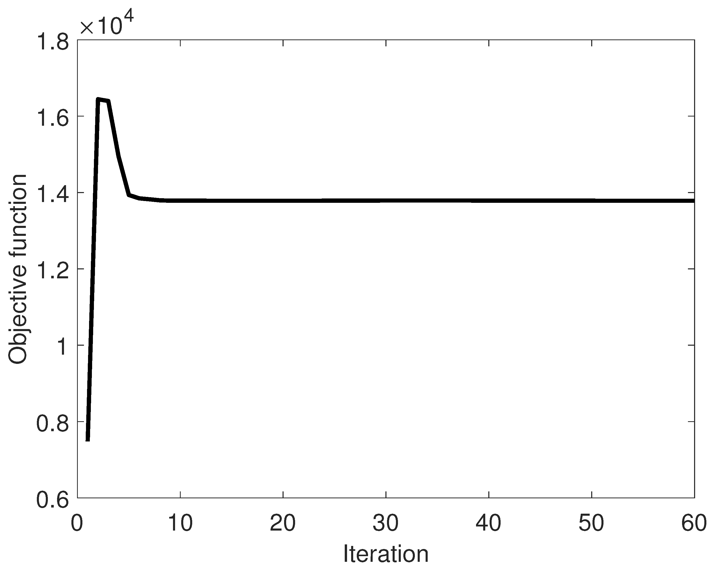
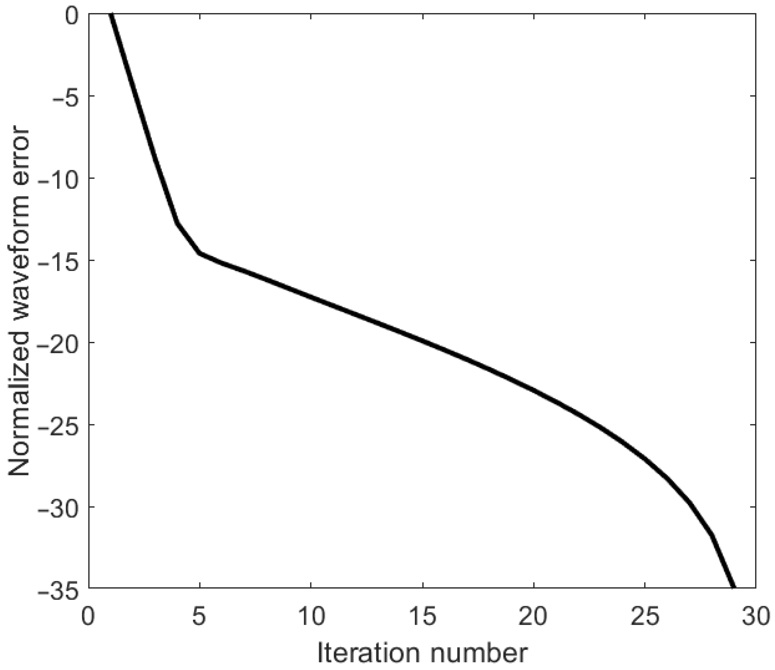
5.3. ADMM Convergence Analysis
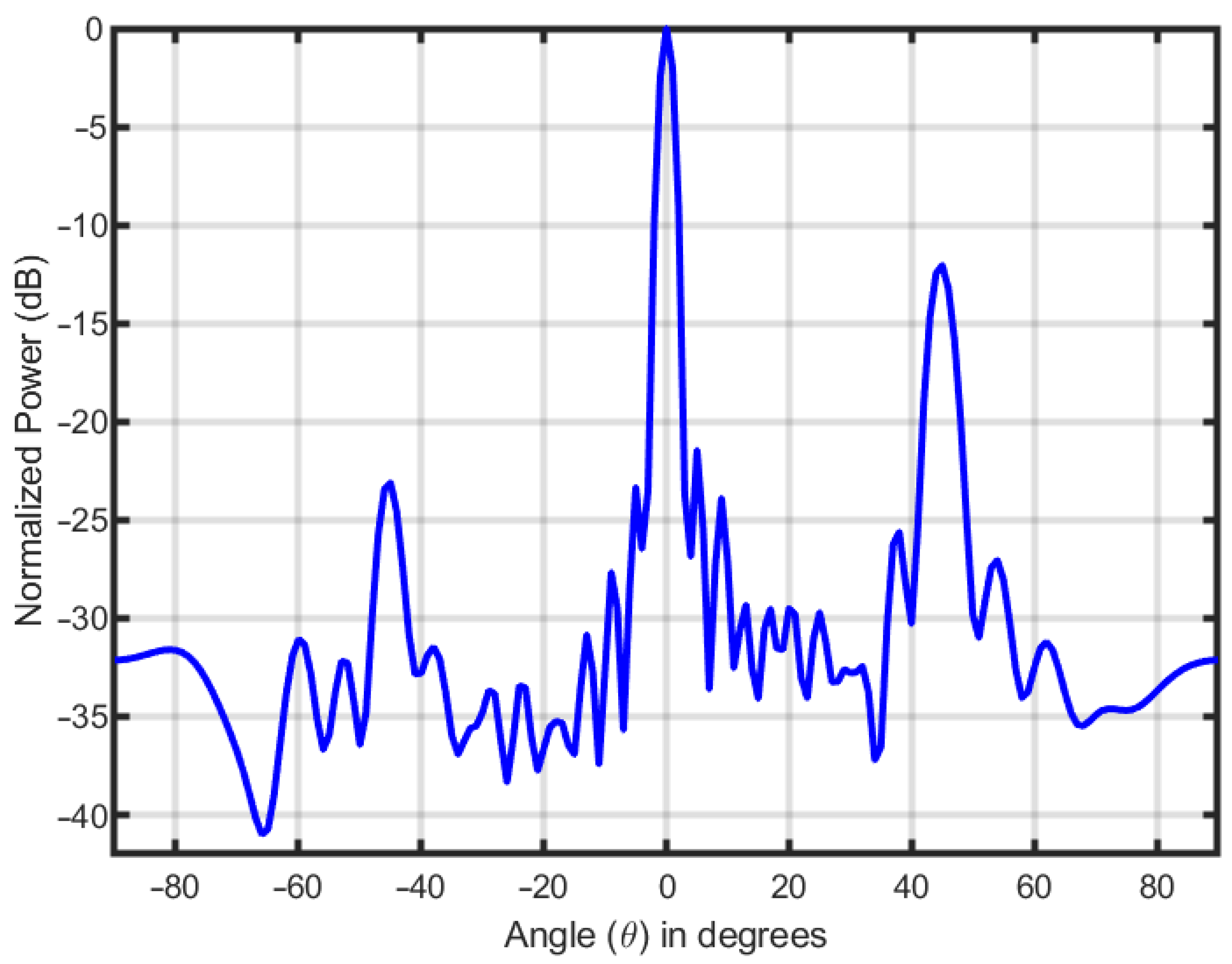
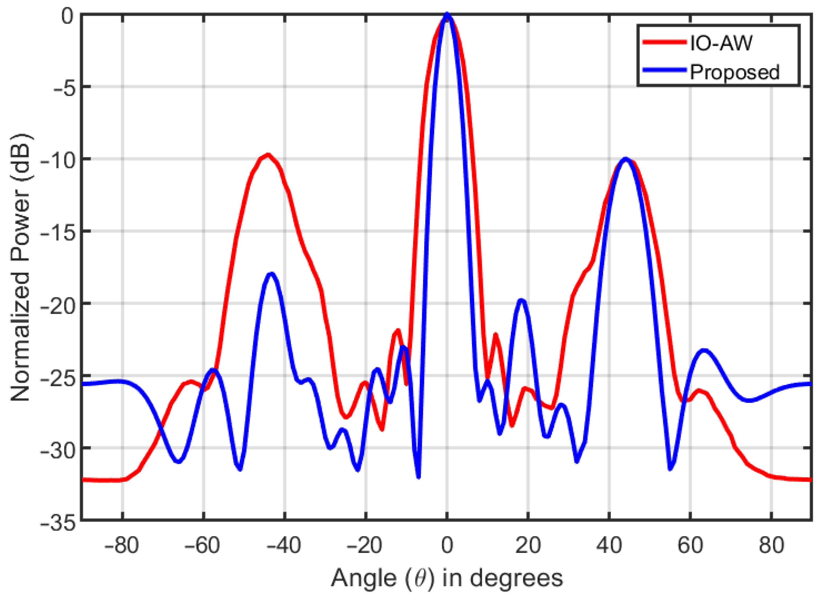
5.4. Beampattern Analysis
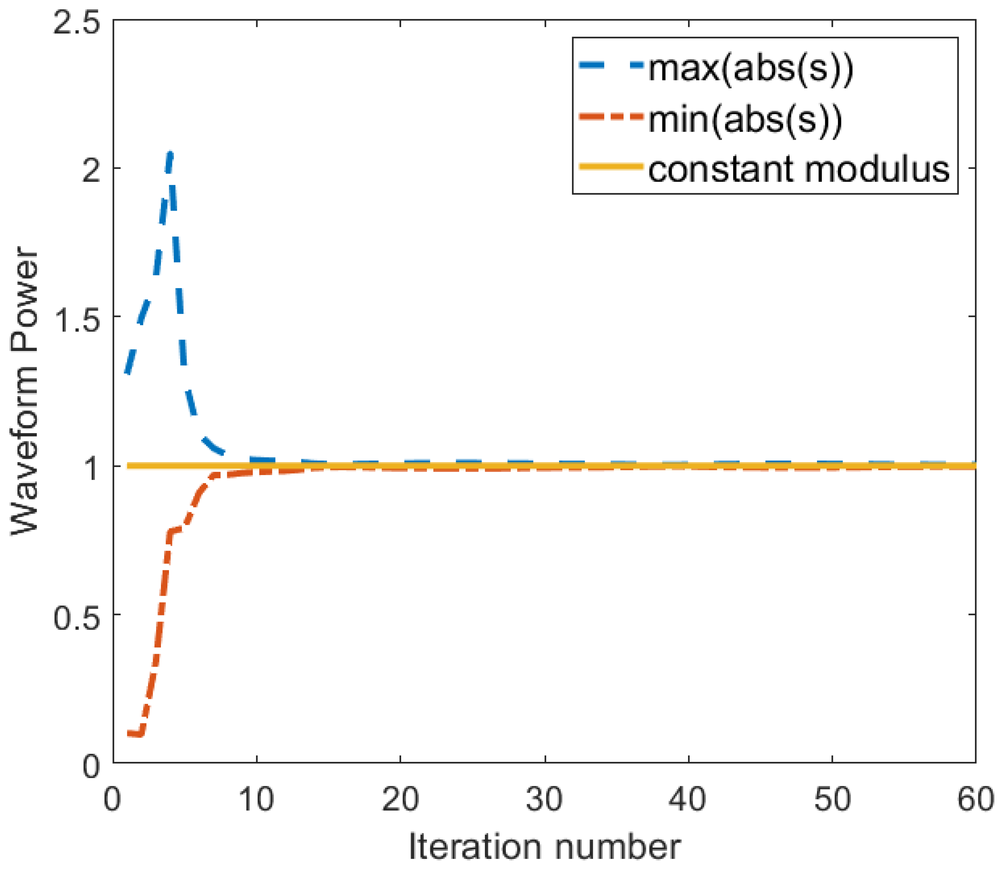
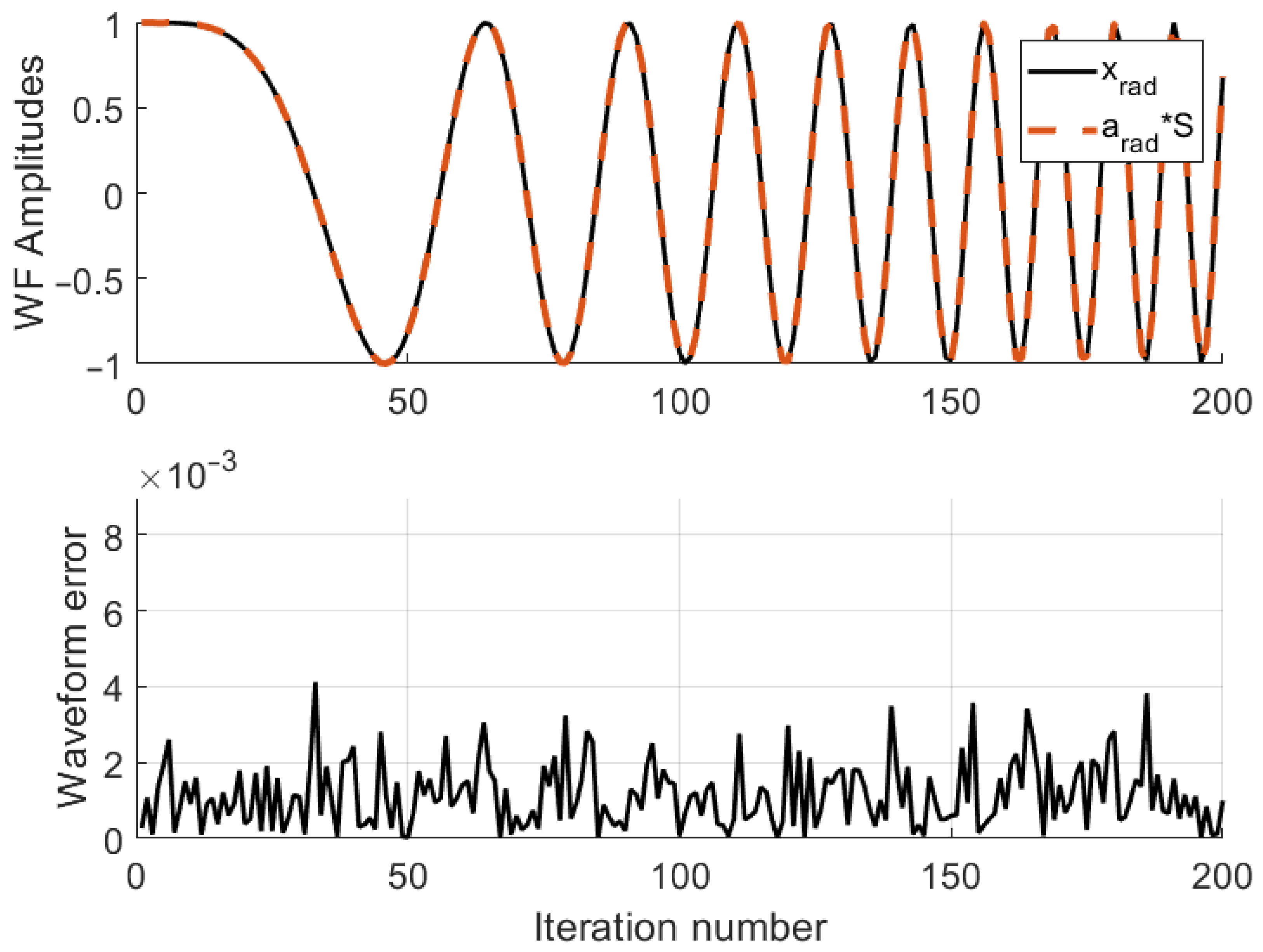
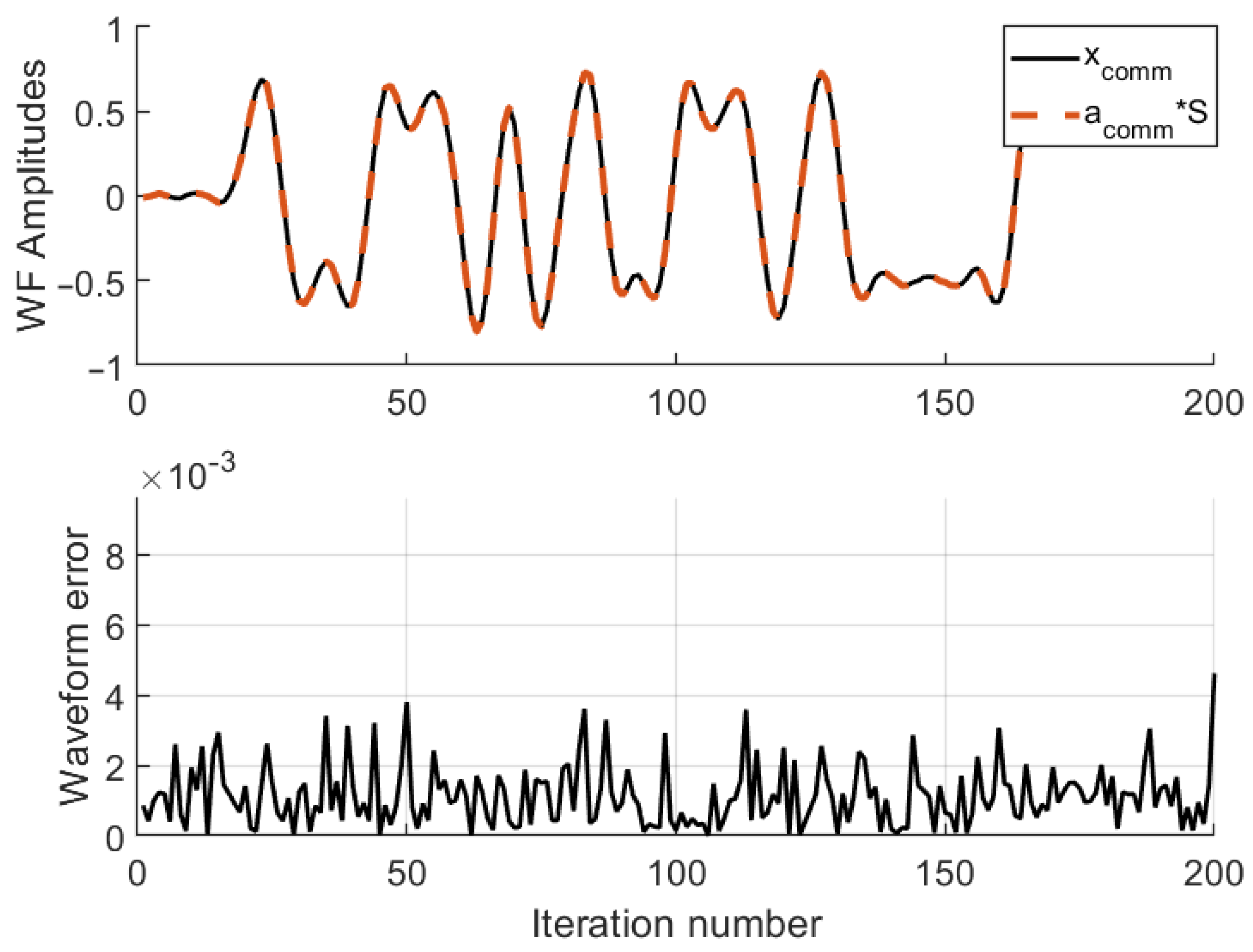
5.5. Waveform Error Analysis
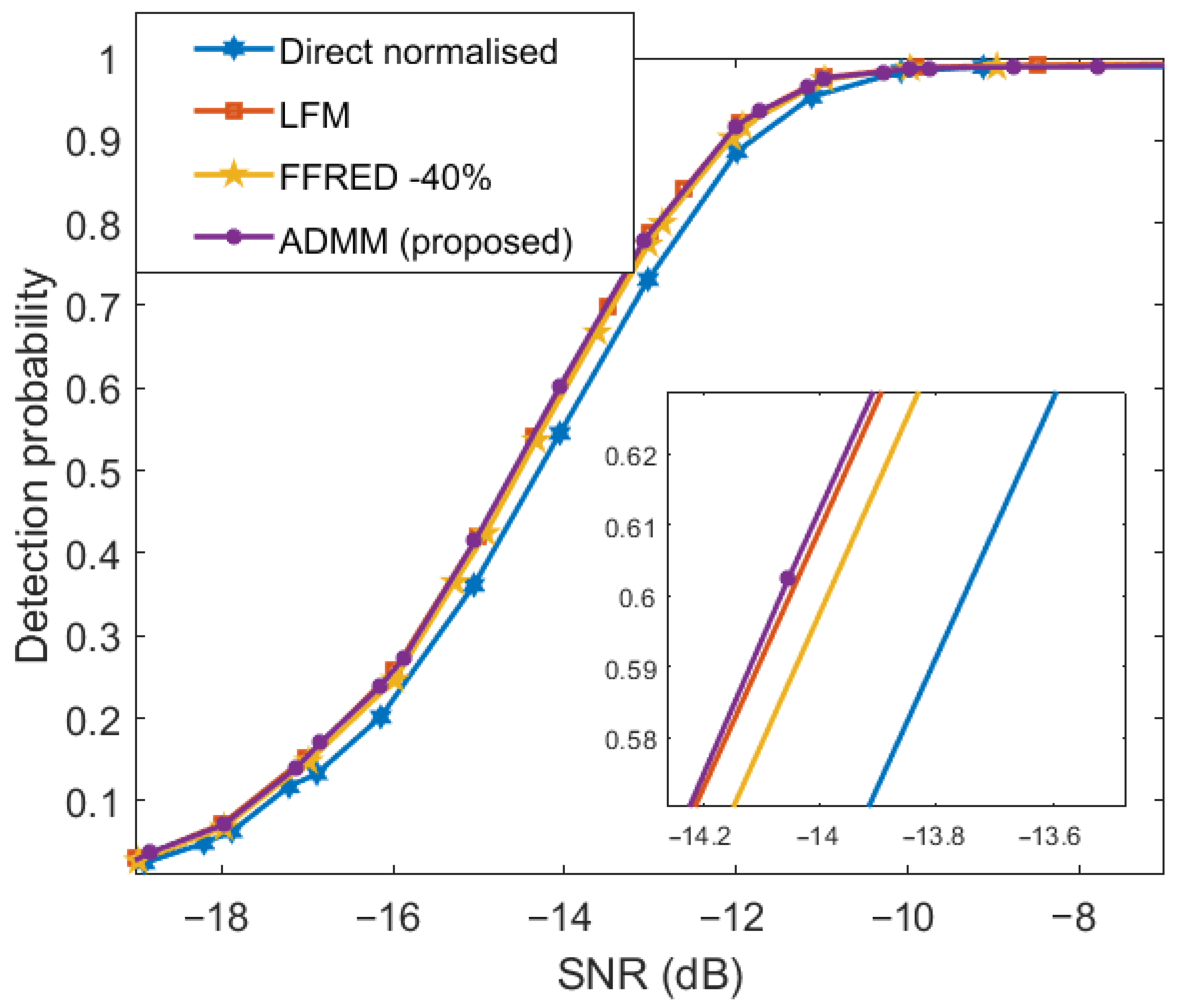
5.6. Radar Performance Analysis
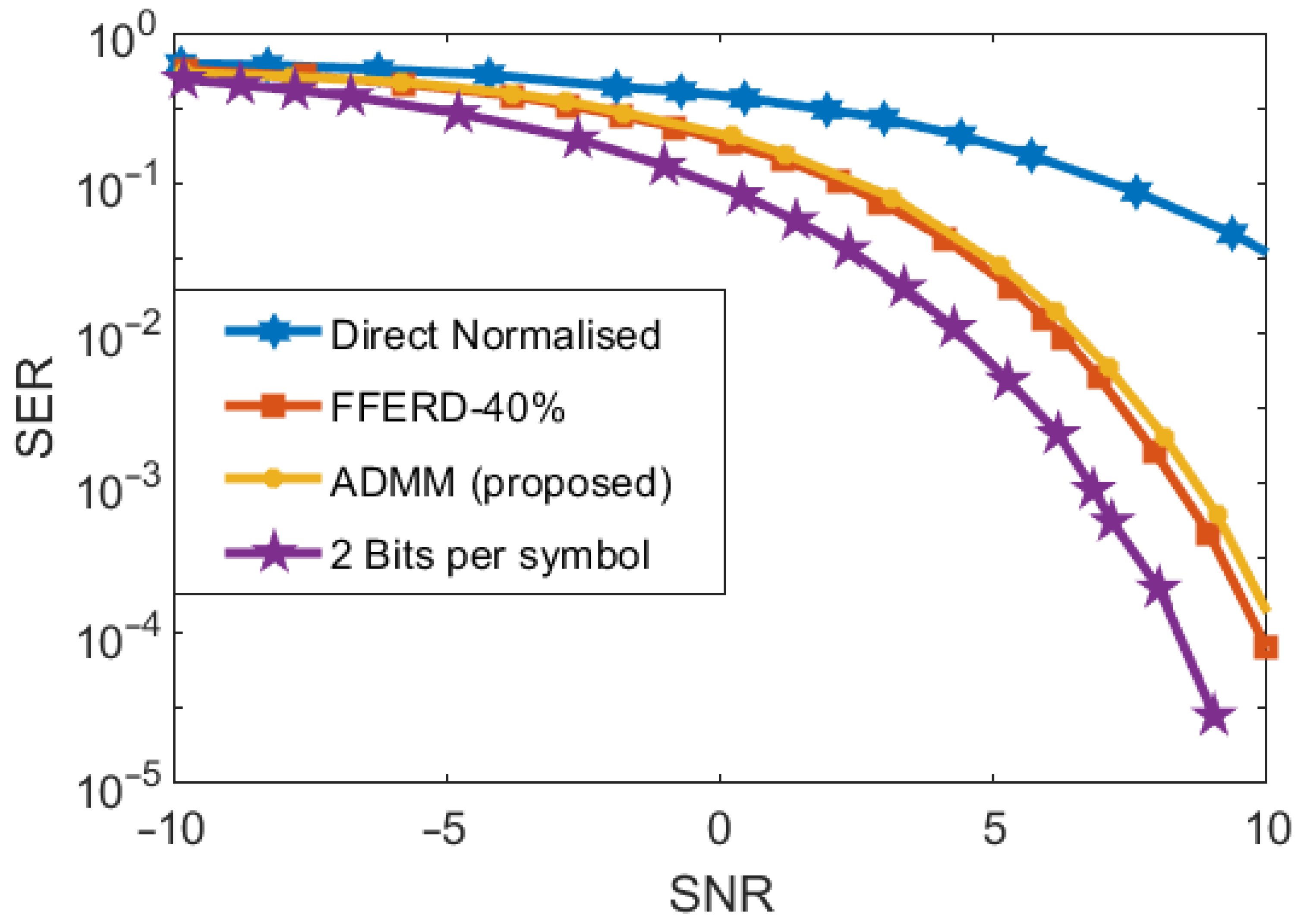
5.7. Communication Performance Analysis
6. Conclusions
Author Contributions
Funding
Institutional Review Board Statement
Data Availability Statement
Conflicts of Interest
References
- Benedetto, F.; Mastroeni, L.; Quaresima, G. Auction-based Theory for Dynamic Spectrum Access: A Review. In Proceedings of the 2021 44th International Conference on Telecommunications and Signal Processing (TSP), Brno, Czech Republic, 26–28 July 2021; pp. 146–151. [Google Scholar]
- Chapin, J.; Lehr, W. Mobile Broadband Growth, Spectrum Scarcity, and Sustainable Competition; TPRC: Denver, CO, USA, 2011. [Google Scholar]
- Noam, E. Spectrum auctions: Yesterday’s heresy, today’s orthodoxy, tomorrow’s anachronism. Taking the next step to open spectrum access. J. Law Econ. 1998, 41, 765–790. [Google Scholar] [CrossRef]
- Martínez-Santos, F.; Frias, Z.; Escribano, Á. What drives spectrum prices in multi-band spectrum markets? An empirical analysis of 4G and 5G auctions in Europe. Appl. Econ. 2022, 54, 536–553. [Google Scholar] [CrossRef]
- Sridhar, V.; Prasad, R. Analysis of spectrum pricing for commercial mobile services: A cross country study. Telecommun. Policy 2021, 45, 102221. [Google Scholar] [CrossRef]
- Cave, M. The Past, Present and Future of Spectrum Auctions. In The Debates Shaping Spectrum Policy; CRC Press: Boca Raton, FL, USA, 2021; pp. 11–27. [Google Scholar]
- Munir, M.F.; Basit, A.; Khan, W.; Saleem, A.; Al-salehi, A. A Comprehensive Study of Past, Present, and Future of Spectrum Sharing and Information Embedding Techniques in Joint Wireless Communication and Radar Systems. Wirel. Commun. Mob. Comput. 2022, 2022. [Google Scholar] [CrossRef]
- Papadias, C.B.; Ratnarajah, T.; Slock, D.T. Spectrum Sharing: The Next Frontier in Wireless Networks; John Wiley & Sons: Hoboken, NJ, USA, 2020. [Google Scholar]
- Cheema, A.A.; Salous, S. Spectrum occupancy measurements and analysis in 2.4 GHz WLAN. Electronics 2019, 8, 1011. [Google Scholar] [CrossRef]
- Cheema, A.A.; Salous, S. Digital FMCW for ultrawideband spectrum sensing. Radio Sci. 2016, 51, 1413–1420. [Google Scholar] [CrossRef]
- Peha, J.M. Approaches to spectrum sharing. IEEE Commun. Mag. 2005, 43, 10–12. [Google Scholar] [CrossRef]
- Mir, S.; Bari, I.; Kamal, M.; Ali, H. Constraint waveform design for spectrum sharing under coexistence of radar and communication systems. IEEE Access 2021, 9, 46093–46105. [Google Scholar] [CrossRef]
- Huang, Y.; Hu, S.; Ma, S.; Liu, Z.; Xiao, M. Designing Low-PAPR Waveform for OFDM-based RadCom Systems. IEEE Trans. Wirel. Commun. 2022, 21, 6979–6993. [Google Scholar] [CrossRef]
- Liu, F.; Cui, Y.; Masouros, C.; Xu, J.; Han, T.X.; Eldar, Y.C.; Buzzi, S. Integrated sensing and communications: Towards dual-functional wireless networks for 6G and beyond. IEEE J. Sel. Areas Commun. 2022, 40, 1728–1767. [Google Scholar] [CrossRef]
- Cheng, X.; Duan, D.; Gao, S.; Yang, L. Integrated Sensing and Communications (ISAC) for Vehicular Communication Networks (VCN). IEEE Internet Things J. 2022, 9, 23441–23451. [Google Scholar] [CrossRef]
- Zheng, L.; Lops, M.; Eldar, Y.C.; Wang, X. Radar and communication coexistence: An overview: A review of recent methods. IEEE Signal Process. Mag. 2019, 36, 85–99. [Google Scholar] [CrossRef]
- Tavik, G.C.; Hilterbrick, C.L.; Evins, J.B.; Alter, J.J.; Crnkovich, J.G.; de Graaf, J.W.; Habicht, W.; Hrin, G.P.; Lessin, S.A.; Wu, D.C.; et al. The advanced multifunction RF concept. IEEE Trans. Microw. Theory Tech. 2005, 53, 1009–1020. [Google Scholar] [CrossRef]
- Moghaddasi, J.; Wu, K. Multifunctional transceiver for future radar sensing and radio communicating data-fusion platform. IEEE Access 2016, 4, 818–838. [Google Scholar] [CrossRef]
- Hassanien, A.; Amin, M.G.; Aboutanios, E.; Himed, B. Dual-function radar communication systems: A solution to the spectrum congestion problem. IEEE Signal Process. Mag. 2019, 36, 115–126. [Google Scholar] [CrossRef]
- Tsinos, C.G.; Arora, A.; Chatzinotas, S.; Ottersten, B. Joint transmit waveform and receive filter design for dual-function radar-communication systems. IEEE J. Sel. Top. Signal Process. 2021, 15, 1378–1392. [Google Scholar] [CrossRef]
- Wen, C.; Huang, Y.; Davidson, T.N. Efficient Transceiver Design for MIMO Dual-Function Radar-Communication Systems. IEEE Trans. Signal Process. 2023, 71, 1786–1801. [Google Scholar] [CrossRef]
- Rong, J.; Liu, F.; Miao, Y. Integrated Radar and Communications Waveform Design Based on Multi-Symbol OFDM. Remote Sens. 2022, 14, 4705. [Google Scholar] [CrossRef]
- Chiriyath, A.R.; Paul, B.; Bliss, D.W. Radar-communications convergence: Coexistence, cooperation, and co-design. IEEE Trans. Cogn. Commun. Netw. 2017, 3, 1–12. [Google Scholar] [CrossRef]
- Singh, R.; Saluja, D.; Kumar, S. R-Comm: A traffic based approach for joint vehicular radar-communication. IEEE Trans. Intell. Veh. 2021, 7, 83–92. [Google Scholar] [CrossRef]
- Ma, D.; Shlezinger, N.; Huang, T.; Liu, Y.; Eldar, Y.C. Joint radar-communication strategies for autonomous vehicles: Combining two key automotive technologies. IEEE Signal Process. Mag. 2020, 37, 85–97. [Google Scholar] [CrossRef]
- Han, L.; Wu, K. 24-GHz integrated radio and radar system capable of time-agile wireless communication and sensing. IEEE Trans. Microw. Theory Tech. 2012, 60, 619–631. [Google Scholar] [CrossRef]
- Kang, B.; Aldayel, O.; Monga, V.; Rangaswamy, M. Spatio-spectral radar beampattern design for coexistence with wireless communication systems. IEEE Trans. Aerosp. Electron. Syst. 2018, 55, 644–657. [Google Scholar] [CrossRef]
- Sodagari, S.; Khawar, A.; Clancy, T.C.; McGwier, R. A projection based approach for radar and telecommunication systems coexistence. In Proceedings of the 2012 IEEE Global Communications Conference (GLOBECOM), Anaheim, CA, USA, 3–7 December 2012; pp. 5010–5014. [Google Scholar]
- Babaei, A.; Tranter, W.H.; Bose, T. A nullspace-based precoder with subspace expansion for radar/communications coexistence. In Proceedings of the 2013 IEEE Global Communications Conference (GLOBECOM), Atlanta, GA, USA, 9–13 December 2013; pp. 3487–3492. [Google Scholar]
- Mahal, J.A.; Khawar, A.; Abdelhadi, A.; Clancy, T.C. Spectral coexistence of MIMO radar and MIMO cellular system. IEEE Trans. Aerosp. Electron. Syst. 2017, 53, 655–668. [Google Scholar] [CrossRef]
- Li, B.; Petropulu, A.P. Joint transmit designs for coexistence of MIMO wireless communications and sparse sensing radars in clutter. IEEE Trans. Aerosp. Electron. Syst. 2017, 53, 2846–2864. [Google Scholar] [CrossRef]
- Li, B.; Petropulu, A.P.; Trappe, W. Optimum co-design for spectrum sharing between matrix completion based MIMO radars and a MIMO communication system. IEEE Trans. Signal Process. 2016, 64, 4562–4575. [Google Scholar] [CrossRef]
- Zhu, J.; Cui, Y.; Mu, J.; Jing, X. OFDM-based Dual-Function Radar-Communications: Optimal Resource Allocation for Fairness. In Proceedings of the 2022 IEEE 95th Vehicular Technology Conference:(VTC2022-Spring), Helsinki, Finland, 19–22 June 2022; pp. 1–5. [Google Scholar]
- Johnston, J.; Venturino, L.; Grossi, E.; Lops, M.; Wang, X. MIMO OFDM dual-function radar-communication under error rate and beampattern constraints. IEEE J. Sel. Areas Commun. 2022, 40, 1951–1964. [Google Scholar] [CrossRef]
- Ahmed, A.; Zhang, Y.D.; Hassanien, A. Joint radar-communications exploiting optimized OFDM waveforms. Remote Sens. 2021, 13, 4376. [Google Scholar] [CrossRef]
- Xu, Z.; Petropulu, A. A wideband dual function radar communication system with sparse array and ofdm waveforms. arXiv 2021, arXiv:2106.05878. [Google Scholar]
- Liu, Y.; Liao, G.; Chen, Y.; Xu, J.; Yin, Y. Super-resolution range and velocity estimations with OFDM integrated radar and communications waveform. IEEE Trans. Veh. Technol. 2020, 69, 11659–11672. [Google Scholar] [CrossRef]
- Liu, Y.; Liao, G.; Yang, Z. Robust OFDM integrated radar and communications waveform design based on information theory. Signal Process. 2019, 162, 317–329. [Google Scholar] [CrossRef]
- Wen, C.; Huang, Y.; Zheng, L.; Liu, W.; Davidson, T.N. Transmit Waveform Design for Dual-Function Radar-Communication Systems via Hybrid Linear-Nonlinear Precoding. IEEE Trans. Signal Process. 2023, 71, 2130–2145. [Google Scholar] [CrossRef]
- Nowak, M.J.; Zhang, Z.; LoMonte, L.; Wicks, M.; Wu, Z. Mixed-modulated linear frequency modulated radar-communications. IET Radar Sonar Navig. 2017, 11, 313–320. [Google Scholar] [CrossRef]
- Zhang, Y.; Li, Q.; Huang, L.; Dai, K.; Song, J. Waveform design for joint radar-communication with nonideal power amplifier and outband interference. In Proceedings of the 2017 IEEE Wireless Communications and Networking Conference (WCNC), San Francisco, CA, USA, 19–22 March 2017; pp. 1–6. [Google Scholar]
- Hassanien, A.; Amin, M.G.; Zhang, Y.D.; Ahmad, F. Phase-modulation based dual-function radar-communications. IET Radar Sonar Navig. 2016, 10, 1411–1421. [Google Scholar] [CrossRef]
- Hassanien, A.; Amin, M.G.; Zhang, Y.D.; Ahmad, F. Dual-function radar-communications: Information embedding using sidelobe control and waveform diversity. IEEE Trans. Signal Process. 2015, 64, 2168–2181. [Google Scholar] [CrossRef]
- Ahmed, A.; Zhang, Y.D.; Gu, Y. Dual-function radar-communications using QAM-based sidelobe modulation. Digit. Signal Process. 2018, 82, 166–174. [Google Scholar] [CrossRef]
- Tang, B.; Stoica, P. MIMO multifunction RF systems: Detection performance and waveform design. IEEE Trans. Signal Process. 2022, 70, 4381–4394. [Google Scholar] [CrossRef]
- Jiang, M.; Liao, G.; Yang, Z.; Liu, Y.; Chen, Y. Integrated radar and communication waveform design based on a shared array. Signal Process. 2021, 182, 107956. [Google Scholar] [CrossRef]
- Liu, X.; Huang, T.; Liu, Y.; Zhou, J. Constant Modulus Waveform Design for Joint Multiuser MIMO Communication and MIMO Radar. In Proceedings of the 2021 IEEE Wireless Communications and Networking Conference Workshops (WCNCW), Nanjing, China, 29 March 2021; pp. 1–5. [Google Scholar]
- Mancuso, V.; Alouf, S. Reducing costs and pollution in cellular networks. IEEE Commun. Mag. 2011, 49, 63–71. [Google Scholar] [CrossRef]
- De Maio, A.; De Nicola, S.; Huang, Y.; Luo, Z.Q.; Zhang, S. Design of phase codes for radar performance optimization with a similarity constraint. IEEE Trans. Signal Process. 2008, 57, 610–621. [Google Scholar] [CrossRef]
- Cui, G.; Li, H.; Rangaswamy, M. MIMO radar waveform design with constant modulus and similarity constraints. IEEE Trans. Signal Process. 2013, 62, 343–353. [Google Scholar] [CrossRef]
- Liu, F.; Masouros, C.; Amadori, P.V.; Sun, H. An efficient manifold algorithm for constructive interference based constant envelope precoding. IEEE Signal Process. Lett. 2017, 24, 1542–1546. [Google Scholar] [CrossRef]
- Wang, X.; Hassanien, A.; Amin, M.G. Dual-function MIMO radar communications system design via sparse array optimization. IEEE Trans. Aerosp. Electron. Syst. 2018, 55, 1213–1226. [Google Scholar] [CrossRef]
- Liu, F.; Zhou, L.; Masouros, C.; Li, A.; Luo, W.; Petropulu, A. Toward dual-functional radar-communication systems: Optimal waveform design. IEEE Trans. Signal Process. 2018, 66, 4264–4279. [Google Scholar] [CrossRef]
- Boyd, S.; Parikh, N.; Chu, E.; Peleato, B.; Eckstein, J. Distributed optimization and statistical learning via the alternating direction method of multipliers. Found. Trends® Mach. Learn. 2011, 3, 1–122. [Google Scholar]
- Hong, M.; Luo, Z.Q.; Razaviyayn, M. Convergence analysis of alternating direction method of multipliers for a family of nonconvex problems. SIAM J. Optim. 2016, 26, 337–364. [Google Scholar] [CrossRef]
- McCormick, P.; Blunt, S.; Metcalf, J. Simultaneous radar and communications emissions from a common aperture, part I: Theory. In Proceedings of the 2017 IEEE Radar Conference (RadarConf), Seattle, WA, USA, 8–12 May 2017; pp. 1685–1690. [Google Scholar]


| Abbreviation | Description |
|---|---|
| ADMM | Alternating Direction Method of Multipliers |
| ALM | Augmented Lagrangian Method |
| ATC | Air Traffic Control |
| BER | Bit Error Rate |
| CM | Constant Modulus |
| CMC | Constant Modulus Constraint |
| CRSS | Communication-Radar Spectrum Sharing |
| DFRC | Dual-Function Radar Communication |
| EW | Electronic Warfare |
| FANET | Flying Ad hoc Network |
| FFRED | Far-Field Radiated Emission Design |
| GA | Genetic Algorithm |
| IO-AW | Iterative Optimization with Amplitude Weighting |
| IRCS | Integrated Radar and Communication System |
| ISAC | Integrated Sensing and Communication |
| LFM | Linear Frequency Modulation |
| MIMO | Multi-Input Multi-Output |
| OFDM | Orthogonal Frequency Division Multiplex |
| PAPR | Peak-to-Average Power Ratio |
| PRI | Pulse Repetition Interval |
| QPSK | Quadrature Phase-Shift Keying |
| RCC | Radar-Communication Coexistence |
| SER | Symbol Error Rate |
| ULA | Uniform Linear Array |
| WS | Waveform Synthesis |
| Symbol | Dimension | Description |
|---|---|---|
| M | Number of antennas | |
| N | Number of samples | |
| K | Number of sidelobes | |
| d | Antenna inter-element spacing | |
| Identity matrix | ||
| Wavelength | ||
| nth sample of a discrete waveform | ||
| nth samples of the waveforms transmitted by all antennas | ||
| Space-time transmit waveform matrix | ||
| Vector version of | ||
| Real-valued version of | ||
| Desired radar waveform | ||
| Desired communication waveform | ||
| Combination of desired communication waveform as a matrix | ||
| Vector version of | ||
| Real-valued version of | ||
| Steering vector in radar direction | ||
| Steering vector in communication direction | ||
| Combination of and | ||
| Vector version of | ||
| Real-valued version of | ||
| Combination of sidelobe steering vectors | ||
| Vector version of | ||
| Real-valued version of | ||
| u | Dual variable | |
| v | Dual variable | |
| w | Dual variable | |
| , | Positive constants | |
| , , | Penalty parameters |
| Method | Waveform Modulus | Normalized Waveform Error/dB |
|---|---|---|
| FFRED-0% | Non-constant | −320.08 |
| FFRED-10% | Constant | −34.08 |
| FFRED-40% | Constant | −113.56 |
| MNO | Non-constant | −312.06 |
| IO | Constant | −39.40 |
| IO-AW | Constant | −40.90 |
| ADMM-based (Proposed) | Constant | −35 |
Disclaimer/Publisher’s Note: The statements, opinions and data contained in all publications are solely those of the individual author(s) and contributor(s) and not of MDPI and/or the editor(s). MDPI and/or the editor(s) disclaim responsibility for any injury to people or property resulting from any ideas, methods, instructions or products referred to in the content. |
© 2023 by the authors. Licensee MDPI, Basel, Switzerland. This article is an open access article distributed under the terms and conditions of the Creative Commons Attribution (CC BY) license (https://creativecommons.org/licenses/by/4.0/).
Share and Cite
Saleem, A.; Basit, A.; Munir, M.F.; Waseem, A.; Khan, W.; Malik, A.N.; AlQahtani, S.A.; Daraz, A.; Pathak, P. Alternating Direction Method of Multipliers-Based Constant Modulus Waveform Design for Dual-Function Radar-Communication Systems. Entropy 2023, 25, 1027. https://doi.org/10.3390/e25071027
Saleem A, Basit A, Munir MF, Waseem A, Khan W, Malik AN, AlQahtani SA, Daraz A, Pathak P. Alternating Direction Method of Multipliers-Based Constant Modulus Waveform Design for Dual-Function Radar-Communication Systems. Entropy. 2023; 25(7):1027. https://doi.org/10.3390/e25071027
Chicago/Turabian StyleSaleem, Ahmed, Abdul Basit, Muhammad Fahad Munir, Athar Waseem, Wasim Khan, Aqdas Naveed Malik, Salman A. AlQahtani, Amil Daraz, and Pranavkumar Pathak. 2023. "Alternating Direction Method of Multipliers-Based Constant Modulus Waveform Design for Dual-Function Radar-Communication Systems" Entropy 25, no. 7: 1027. https://doi.org/10.3390/e25071027
APA StyleSaleem, A., Basit, A., Munir, M. F., Waseem, A., Khan, W., Malik, A. N., AlQahtani, S. A., Daraz, A., & Pathak, P. (2023). Alternating Direction Method of Multipliers-Based Constant Modulus Waveform Design for Dual-Function Radar-Communication Systems. Entropy, 25(7), 1027. https://doi.org/10.3390/e25071027