

Optimizing Quantum Classification Algorithms on Classical Benchmark Datasets

 , , , and
Abstract
1. Introduction
2. Materials and Methods
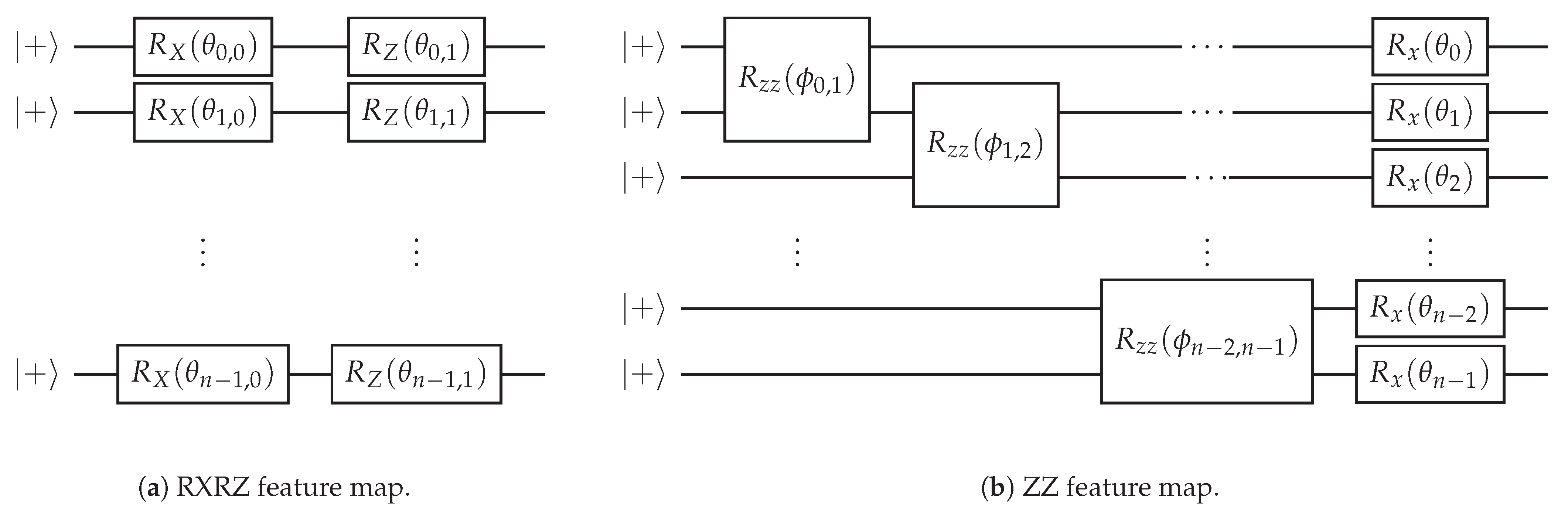
2.1. Quantum Classification Algorithms and Quantum Embeddings
2.2. Quantum Fidelity and RBF Fidelity Classifiers
2.3. Quantum Metric Learning
2.4. Datasets
3. Results
3.1. Pre-Processing
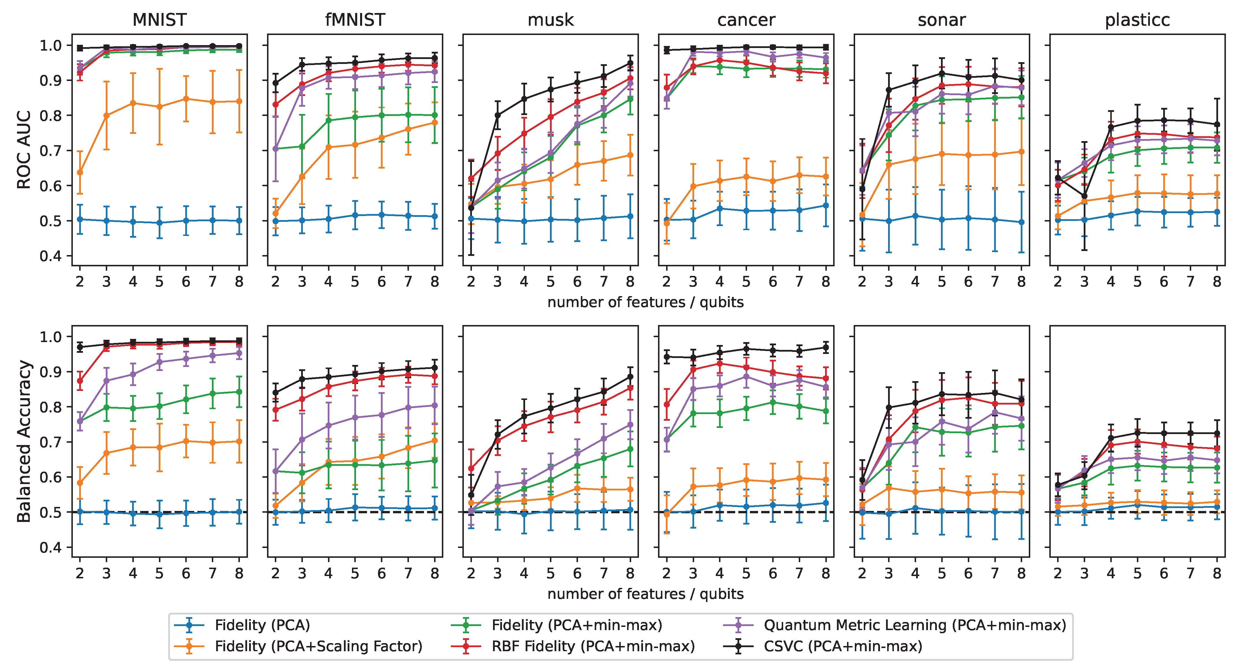
3.2. Classification
4. Discussion and Conclusions
Author Contributions
Funding
Data Availability Statement
Acknowledgments
Conflicts of Interest
Appendix A. Performance Metrics
- true positives (TP)—number of positive samples classified as positive
- false positives (FP)—number of negative samples classified as positive
- true negatives (TN)—number of negative samples classified as negative
- false negatives (FN)—number of positive samples classified as negative
References
- Biamonte, J.; Wittek, P.; Pancotti, N.; Rebentrost, P.; Wiebe, N.; Lloyd, S. Quantum machine learning. Nature 2017, 549, 195–202. [Google Scholar] [CrossRef] [PubMed]
- Cerezo, M.; Verdon, G.; Huang, H.Y.; Cincio, L.; Coles, P.J. Challenges and opportunities in quantum machine learning. Nat. Comput. Sci. 2022, 2, 567–576. [Google Scholar] [CrossRef]
- Grover, L.K. A fast quantum mechanical algorithm for database search. In Proceedings of the Twenty-Eighth Annual ACM Symposium on Theory of Computing, Philadelphia, PA, USA, 22–24 May 1996; pp. 212–219. [Google Scholar]
- Durr, C.; Hoyer, P. A quantum algorithm for finding the minimum. arXiv 1996, arXiv:quant-ph/9607014. [Google Scholar]
- Farhi, E.; Goldstone, J.; Gutmann, S.; Lapan, J.; Lundgren, A.; Preda, D. A quantum adiabatic evolution algorithm applied to random instances of an NP-complete problem. Science 2001, 292, 472–475. [Google Scholar] [CrossRef]
- Harrow, A.W.; Hassidim, A.; Lloyd, S. Quantum Algorithm for Linear Systems of Equations. Phys. Rev. Lett. 2009, 103, 150502. [Google Scholar] [CrossRef]
- Neven, H.; Denchev, V.S.; Rose, G.; Macready, W.G. Training a large scale classifier with the quantum adiabatic algorithm. arXiv 2009, arXiv:0912.0779. [Google Scholar]
- Rebentrost, P.; Mohseni, M.; Lloyd, S. Quantum support vector machine for big data classification. Phys. Rev. Lett. 2014, 113, 130503. [Google Scholar] [CrossRef]
- Schuld, M.; Sinayskiy, I.; Petruccione, F. The quest for a Quantum Neural Network. Quantum Inf. Process. 2014, 13, 2567–2586. [Google Scholar] [CrossRef]
- Farhi, E.; Neven, H. Classification with quantum neural networks on near term processors. arXiv 2018, arXiv:1802.06002. [Google Scholar]
- Benedetti, M.; Lloyd, E.; Sack, S.; Fiorentini, M. Parameterized quantum circuits as machine learning models. Quantum Sci. Technol. 2019, 4, 043001. [Google Scholar] [CrossRef]
- Tacchino, F.; Barkoutsos, P.; Macchiavello, C.; Tavernelli, I.; Gerace, D.; Bajoni, D. Quantum implementation of an artificial feed-forward neural network. Quantum Sci. Technol. 2020, 5, 044010. [Google Scholar] [CrossRef]
- Mangini, S.; Tacchino, F.; Gerace, D.; Bajoni, D.; Macchiavello, C. Quantum computing models for artificial neural networks. EPL Europhys. Lett. 2021, 134, 10002. [Google Scholar] [CrossRef]
- Tacchino, F.; Mangini, S.; Barkoutsos, P.K.; Macchiavello, C.; Gerace, D.; Tavernelli, I.; Bajoni, D. Variational Learning for Quantum Artificial Neural Networks. IEEE Trans. Quantum Eng. 2021, 2, 1–10. [Google Scholar] [CrossRef]
- Cerezo, M.; Arrasmith, A.; Babbush, R.; Benjamin, S.C.; Endo, S.; Fujii, K.; McClean, J.R.; Mitarai, K.; Yuan, X.; Cincio, L.; et al. Variational quantum algorithms. Nat. Rev. Phys. 2021, 3, 625–644. [Google Scholar] [CrossRef]
- Abbas, A.; Sutter, D.; Zoufal, C.; Lucchi, A.; Figalli, A.; Woerner, S. The power of quantum neural networks. Nat. Comput. Sci. 2021, 1, 403–409. [Google Scholar] [CrossRef]
- Liu, J.; Najafi, K.; Sharma, K.; Tacchino, F.; Jiang, L.; Mezzacapo, A. Analytic Theory for the Dynamics of Wide Quantum Neural Networks. Phys. Rev. Lett. 2023, 130, 150601. [Google Scholar] [CrossRef]
- Havlíček, V.; Córcoles, A.D.; Temme, K.; Harrow, A.W.; Kandala, A.; Chow, J.M.; Gambetta, J.M. Supervised learning with quantum-enhanced feature spaces. Nature 2019, 567, 209–212. [Google Scholar] [CrossRef]
- Schuld, M.; Killoran, N. Quantum machine learning in feature hilbert spaces. Phys. Rev. Lett. 2019, 122, 040504. [Google Scholar] [CrossRef]
- Lloyd, S.; Schuld, M.; Ijaz, A.; Izaac, J.; Killoran, N. Quantum embeddings for machine learning. arXiv 2020, arXiv:2001.03622. [Google Scholar]
- Liu, Y.; Arunachalam, S.; Temme, K. A rigorous and robust quantum speed-up in supervised machine learning. Nat. Phys. 2021, 17, 1013–1017. [Google Scholar] [CrossRef]
- Peters, E.; Caldeira, J.; Ho, A.; Leichenauer, S.; Mohseni, M.; Neven, H.; Spentzouris, P.; Strain, D.; Perdue, G.N. Machine learning of high dimensional data on a noisy quantum processor. Npj Quantum Inf. 2021, 7, 161. [Google Scholar] [CrossRef]
- Huang, H.Y.; Broughton, M.; Mohseni, M.; Babbush, R.; Boixo, S.; Neven, H.; McClean, J.R. Power of data in quantum machine learning. Nat. Commun. 2021, 12, 2631. [Google Scholar] [CrossRef] [PubMed]
- Jerbi, S.; Fiderer, L.J.; Poulsen Nautrup, H.; Kübler, J.M.; Briegel, H.J.; Dunjko, V. Quantum machine learning beyond kernel methods. Nat. Commun. 2023, 14, 517. [Google Scholar] [CrossRef]
- Wu, S.L.; Sun, S.; Guan, W.; Zhou, C.; Chan, J.; Cheng, C.L.; Pham, T.; Qian, Y.; Wang, A.Z.; Zhang, R.; et al. Application of quantum machine learning using the quantum kernel algorithm on high energy physics analysis at the LHC. Phys. Rev. Res. 2021, 3, 033221. [Google Scholar] [CrossRef]
- Schuhmacher, J.; Boggia, L.; Belis, V.; Puljak, E.; Grossi, M.; Pierini, M.; Vallecorsa, S.; Tacchino, F.; Barkoutsos, P.; Tavernelli, I. Unravelling physics beyond the standard model with classical and quantum anomaly detection. arXiv 2023, arXiv:2301.10787. [Google Scholar]
- Woźniak, K.A.; Belis, V.; Puljak, E.; Barkoutsos, P.; Dissertori, G.; Grossi, M.; Pierini, M.; Reiter, F.; Tavernelli, I.; Vallecorsa, S. Quantum anomaly detection in the latent space of proton collision events at the LHC. arXiv 2023, arXiv:2301.10780. [Google Scholar]
- Sancho-Lorente, T.; Román-Roche, J.; Zueco, D. Quantum kernels to learn the phases of quantum matter. Phys. Rev. A 2022, 105, 042432. [Google Scholar] [CrossRef]
- Grossi, M.; Ibrahim, N.; Radescu, V.; Loredo, R.; Voigt, K.; Von Altrock, C.; Rudnik, A. Mixed Quantum–Classical Method for Fraud Detection With Quantum Feature Selection. IEEE Trans. Quantum Eng. 2022, 3, 1–12. [Google Scholar] [CrossRef]
- Mensa, S.; Sahin, E.; Tacchino, F.; Barkoutsos, P.K.; Tavernelli, I. Quantum machine learning framework for virtual screening in drug discovery: A prospective quantum advantage. Mach. Learn. Sci. Technol. 2023, 4, 015023. [Google Scholar] [CrossRef]
- Li, Y.; Benjamin, S.C. Efficient Variational Quantum Simulator Incorporating Active Error Minimization. Phys. Rev. X 2017, 7, 021050. [Google Scholar] [CrossRef]
- Temme, K.; Bravyi, S.; Gambetta, J.M. Error Mitigation for Short-Depth Quantum Circuits. Phys. Rev. Lett. 2017, 119. [Google Scholar] [CrossRef] [PubMed]
- Endo, S.; Benjamin, S.C.; Li, Y. Practical Quantum Error Mitigation for Near-Future Applications. Phys. Rev. X 2018, 8, 031027. [Google Scholar] [CrossRef]
- Earnest, N.; Tornow, C.; Egger, D.J. Pulse-efficient circuit transpilation for quantum applications on cross-resonance-based hardware. Phys. Rev. Res. 2021, 3, 043088. [Google Scholar] [CrossRef]
- Kim, Y.; Wood, C.J.; Yoder, T.J.; Merkel, S.T.; Gambetta, J.M.; Temme, K.; Kandala, A. Scalable error mitigation for noisy quantum circuits produces competitive expectation values. Nat. Phys. 2023, 19, 752–759. [Google Scholar] [CrossRef]
- Melo, A.; Earnest-Noble, N.; Tacchino, F. Pulse-efficient quantum machine learning. arXiv 2022, arXiv:2211.01383. [Google Scholar]
- McClean, J.R.; Boixo, S.; Smelyanskiy, V.N.; Babbush, R.; Neven, H. Barren plateaus in quantum neural network training landscapes. Nat. Commun. 2018, 9, 4812. [Google Scholar] [CrossRef]
- Cerezo, M.; Sone, A.; Volkoff, T.; Cincio, L.; Coles, P.J. Cost function dependent barren plateaus in shallow parametrized quantum circuits. Nat. Commun. 2021, 12, 1791. [Google Scholar] [CrossRef]
- Thanasilp, S.; Wang, S.; Nghiem, N.A.; Coles, P.J.; Cerezo, M. Subtleties in the trainability of quantum machine learning models. arXiv 2021, arXiv:2110.14753. [Google Scholar] [CrossRef]
- Kübler, J.; Buchholz, S.; Schölkopf, B. The inductive bias of quantum kernels. Adv. Neural Inf. Process. Syst. 2021, 34, 12661–12673. [Google Scholar]
- Shaydulin, R.; Wild, S.M. Importance of kernel bandwidth in quantum machine learning. Phys. Rev. A 2022, 106, 042407. [Google Scholar] [CrossRef]
- Canatar, A.; Peters, E.; Pehlevan, C.; Wild, S.M.; Shaydulin, R. Bandwidth enables generalization in quantum kernel models. arXiv 2022, arXiv:2206.06686. [Google Scholar]
- Thanasilp, S.; Wang, S.; Cerezo, M.; Holmes, Z. Exponential concentration and untrainability in quantum kernel methods. arXiv 2022, arXiv:2208.11060. [Google Scholar]
- Glick, J.R.; Gujarati, T.P.; Corcoles, A.D.; Kim, Y.; Kandala, A.; Gambetta, J.M.; Temme, K. Covariant quantum kernels for data with group structure. arXiv 2021, arXiv:2105.03406. [Google Scholar]
- Shashua, A. Introduction to machine learning: Class notes 67577. arXiv 2009, arXiv:0904.3664. [Google Scholar]
- Farhi, E.; Harrow, A.W. Quantum Supremacy through the Quantum Approximate Optimization Algorithm. arXiv 2019, arXiv:1602.07674. [Google Scholar]
- Barenco, A.; Berthiaume, A.; Deutsch, D.; Ekert, A.; Jozsa, R.; Macchiavello, C. Stabilization of quantum computations by symmetrization. SIAM J. Comput. 1997, 26, 1541–1557. [Google Scholar] [CrossRef]
- Deng, L. The mnist database of handwritten digit images for machine learning research. IEEE Signal Process. Mag. 2012, 29, 141–142. [Google Scholar] [CrossRef]
- Xiao, H.; Rasul, K.; Vollgraf, R. Fashion-mnist: A novel image dataset for benchmarking machine learning algorithms. arXiv 2017, arXiv:1708.07747. [Google Scholar]
- Dietterich, T.G.; Lathrop, R.H.; Lozano-Pérez, T. Solving the multiple instance problem with axis-parallel rectangles. Artif. Intell. 1997, 89, 31–71. [Google Scholar] [CrossRef]
- Romano, J.D.; Le, T.T.; La Cava, W.; Gregg, J.T.; Goldberg, D.J.; Chakraborty, P.; Ray, N.L.; Himmelstein, D.; Fu, W.; Moore, J.H. PMLB v1. 0: An open-source dataset collection for benchmarking machine learning methods. Bioinformatics 2022, 38, 878–880. [Google Scholar] [CrossRef]
- Gorman, R.P.; Sejnowski, T.J. Analysis of hidden units in a layered network trained to classify sonar targets. Neural Netw. 1988, 1, 75–89. [Google Scholar] [CrossRef]
- Wolberg, W.; Mangasarian, O.; Street, N. Breast Cancer Wisconsin (Diagnostic). In UCI Machine Learning Repository; UCI: Irvine, CA, USA, 1995. [Google Scholar] [CrossRef]
- Kessler, R.; Narayan, G.; Avelino, A.; Bachelet, E.; Biswas, R.; Brown, P.; Chernoff, D.; Connolly, A.; Dai, M.; Daniel, S.; et al. Models and simulations for the photometric LSST astronomical time series classification challenge (PLAsTiCC). Publ. Astron. Soc. Pac. 2019, 131, 094501. [Google Scholar] [CrossRef]
- Jolliffe, I.T. Principal Component Analysis for Special Types of Data; Springer: Berlin/Heidelberg, Germany, 2002. [Google Scholar]


| Dataset | # Features | # Positives | # Negatives | Source | Description |
|---|---|---|---|---|---|
| MNIST | 28 × 28 | 500 | 500 | [48] | Grayscale images of hand-written digits (0’s vs. 9’s) |
| fMNIST | 28 × 28 | 500 | 500 | [49] | Grayscale images of clothing (T-shirts vs. dresses) |
| musk | 166 | 207 | 269 | [50,51] | Molecules occurring in different conformations (musk vs. non-musk) |
| sonar | 60 | 97 | 111 | [51,52] | Sonar signals (bounced off a metal cylinder vs. a roughly cylindrical rock) |
| cancer | 30 | 212 | 357 | [53] | Characteristics of breast cancer tumors (benign vs. malignant) |
| plasticc | 67 | 500 | 500 | [54] | Photometric LSST Astronomical Time-series Classification Challenge dataset. Pre-processed by [22] (type II vs. Ia supernovae) |
Disclaimer/Publisher’s Note: The statements, opinions and data contained in all publications are solely those of the individual author(s) and contributor(s) and not of MDPI and/or the editor(s). MDPI and/or the editor(s) disclaim responsibility for any injury to people or property resulting from any ideas, methods, instructions or products referred to in the content. |
© 2023 by the authors. Licensee MDPI, Basel, Switzerland. This article is an open access article distributed under the terms and conditions of the Creative Commons Attribution (CC BY) license (https://creativecommons.org/licenses/by/4.0/).
Share and Cite
John, M.; Schuhmacher, J.; Barkoutsos, P.; Tavernelli, I.; Tacchino, F. Optimizing Quantum Classification Algorithms on Classical Benchmark Datasets. Entropy 2023, 25, 860. https://doi.org/10.3390/e25060860
John M, Schuhmacher J, Barkoutsos P, Tavernelli I, Tacchino F. Optimizing Quantum Classification Algorithms on Classical Benchmark Datasets. Entropy. 2023; 25(6):860. https://doi.org/10.3390/e25060860
Chicago/Turabian StyleJohn, Manuel, Julian Schuhmacher, Panagiotis Barkoutsos, Ivano Tavernelli, and Francesco Tacchino. 2023. "Optimizing Quantum Classification Algorithms on Classical Benchmark Datasets" Entropy 25, no. 6: 860. https://doi.org/10.3390/e25060860
APA StyleJohn, M., Schuhmacher, J., Barkoutsos, P., Tavernelli, I., & Tacchino, F. (2023). Optimizing Quantum Classification Algorithms on Classical Benchmark Datasets. Entropy, 25(6), 860. https://doi.org/10.3390/e25060860