


Multivariate Time Series Information Bottleneck


Abstract
1. Introduction
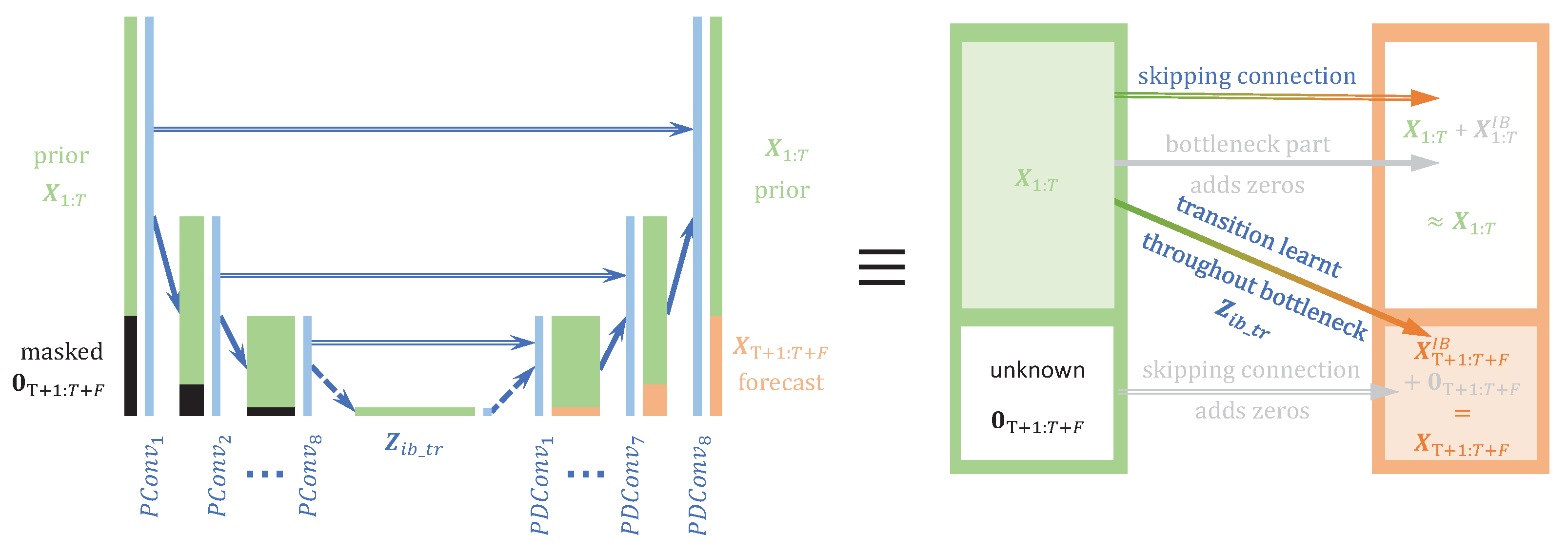
 where is a latent representation, is an encoding part modeled by reducing the time dimension through successive strided convolution layers, and is a decoding part performed by an architecture symmetric to , such that the posterior has the same shape as the prior . U-Net also allows a direct flow of information with an identity mapper between and , also referred to as the skipping layer. This direct flow of information between the prior and the posterior allows for easy reconstruction of the prior image while the information flow through the latent is responsible for the image segmentation objective. Skipping layers are also present between symmetrical hidden layers of the encoder and the decoder. Without the skipping layers, the U-Net is reduced to an autoencoder (AE) structure [32] sketched by the Markov chain acting as a principal component analysis dimensional reduction of in .
2. Methods
2.1. IB-Based Optimal Compression for Time Series Forecasts
2.2. Compression by Source Masking
2.3. Compressing Multi-Dimensional Data by Extreme Spatiotemporal Dimension Reduction
2.4. Performing the Forecast
2.4.1. Decoder
 For this configuration, and under a Laplacian assumption for the distribution , the third term of the IB loss in Equation (8) becomes equivalent to:
 2.4.2. Partial IB Loss with U-Net
2.4.3. IB Interpretation with the Partial Loss
- If we remove the skipping layers, the bottleneck should not only retain the statistics of the transitions from the prior to the posterior but also the reconstruction statistics of the prior.
- If we also remove the source masking of the posterior in , the model is reduced to an autoencoder (AE) and the bottleneck is supposed to perform a dimension reduction of the MTS. Because of the curse of dimensionality, this technique is commonly used to further perform better classifications on the bottleneck representation than on the raw high-dimensional MTS data.
2.5. Proposed Model
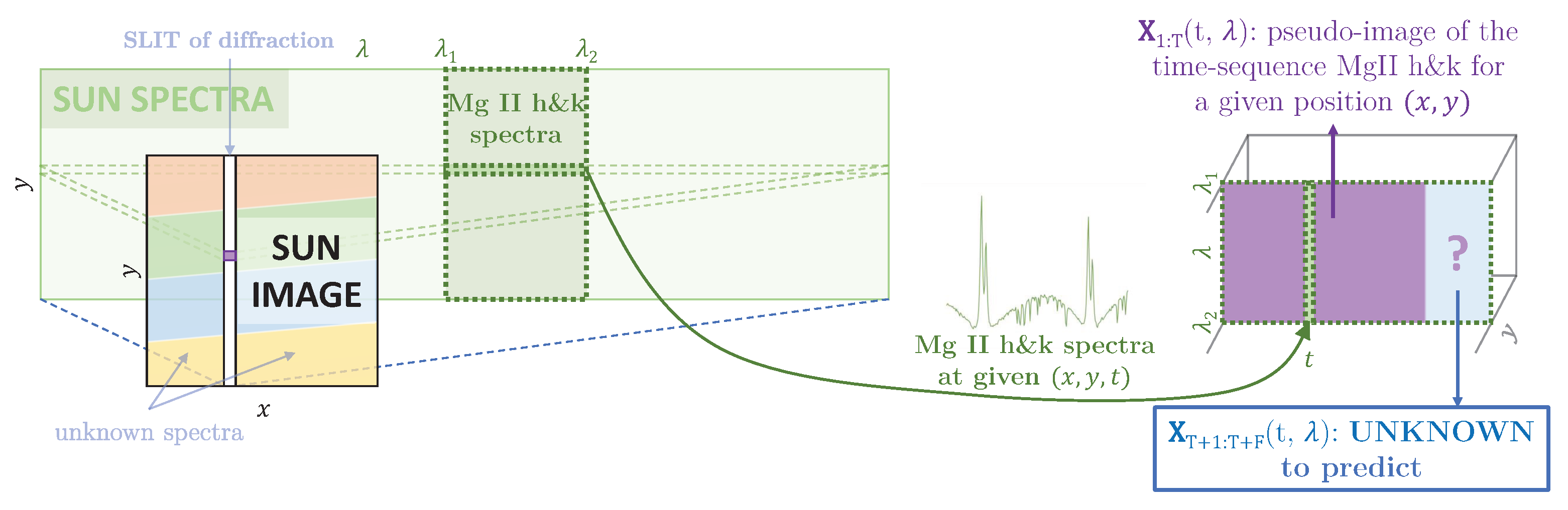
2.6. IRIS Dataset
2.6.1. Problem Formulation
2.6.2. Proposed Approach
2.7. Other MTS Dataset
- AL dataset: The solar power dataset for the year 2006 in Alabama is publicly available (www.nrel.gov/grid/solar-power-data.html, accessed on 20 February 2023). It contains solar power data for 137 solar photovoltaic power plants. Power was sampled every 5 min in the year 2006. Preprocessing was conducted to only extract daily events by ignoring nights when data were zero. At each 5-min interval, the data consisted of vectors with 137 dimensions, and these vectors were normalized by their maximum coordinates. For example, in the case of IRIS data, the maximum value at each time was always set to 1.
- PB dataset: PeMS-BAY data [74] are publicly available (https://zenodo.org/record/5146275#.Y5hF7nbMI2w, accessed on 20 February 2023) and were selected from 325 sensors in the Bay Area of San Francisco by the California State Transportation Agency’s Performance Measurement System [75]. The data represent 6 months of traffic speeds ranging from January 1 to May 31 2017. At each 5-minute interval, the data consist of vectors with 325 dimensions, and these vectors are normalized by their maximum coordinates. For example, in the case of IRIS data, the maximum value at each time was always set to 1.
2.8. Complementary Classifiers to Show Consistency with Applied Sciences
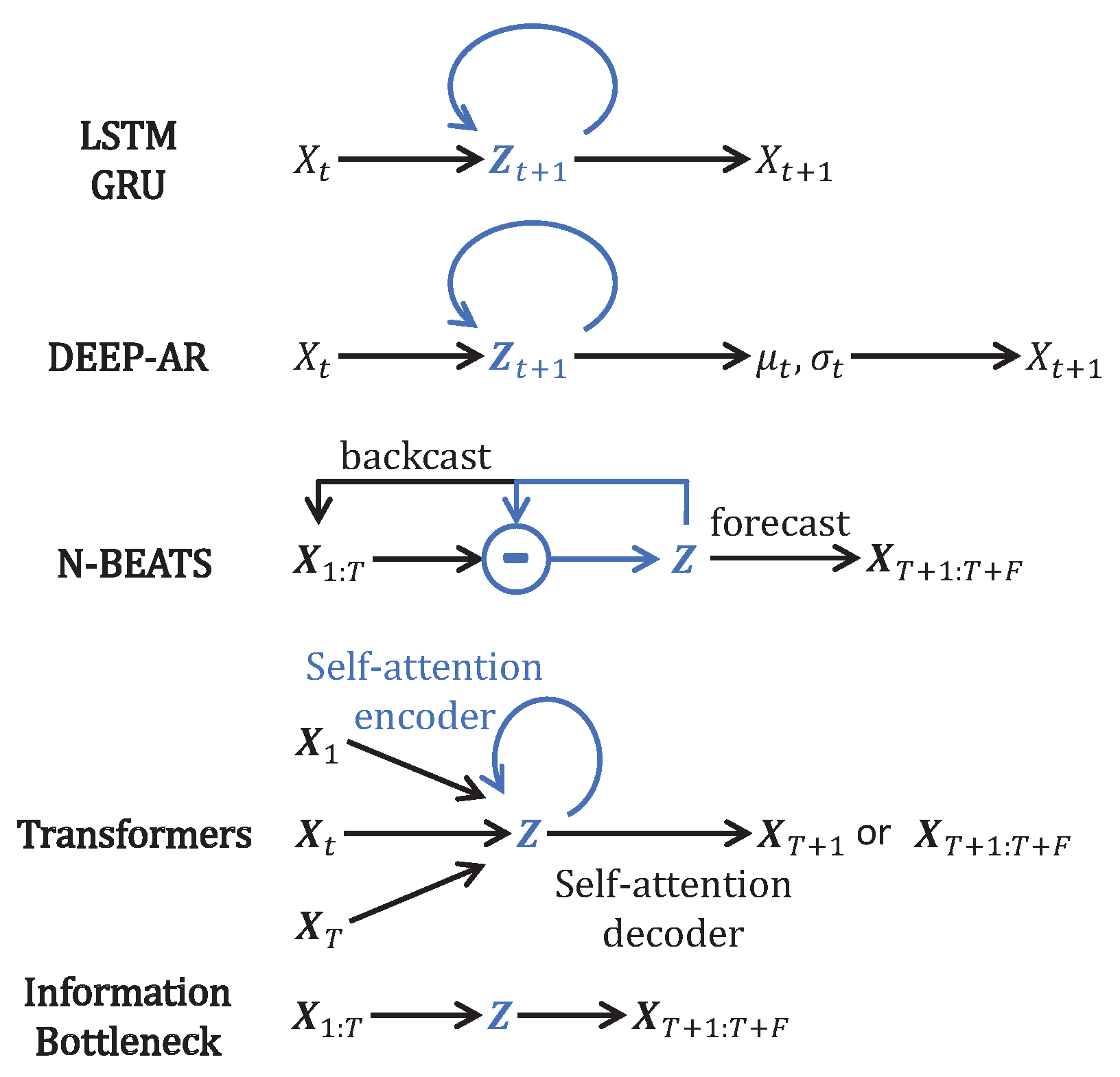
2.9. Comparison with Other Models
- Unique joint spatiotemporal IB: The encoder jointly compresses spatial and temporal dimensions of the prior into a bottleneck with an extreme spatiotemporal dimensional reduction; this is our proposed IB-MTS formulation.
- MTS decomposition model, such as NBeats [3].
- LSTM model: An LSTM cell [6] performs the one-step-ahead forecast and is trained to predict from . It incorporates one layer with M LSTM units. For instance, for the spatiotemporal dimensions of IRIS data, the 180 first time steps are the prior data, and the 60 last time steps are the posterior data to forecast. This model is designed with 240 spatial LSTM/GRU units looped 180 times and all of the cell outputs are returned by the model using TensorFlow option . This layer returns a output and only the last 60 time steps are kept. Moreover, a source masking of the posterior is applied to the input and an identity skipping layer is added to transmit the prior to the output at the same temporal positions in , such that the LSTM layer only accounts for predicting the posterior part . The number of units is directly determined by the shape of the input and output data. Details of the architecture are given in the Appendix B, Table A3.
- GRU model: A GRU [15] cell is trained to predict from . The structure and number of units are the same, similar to the LSTM models, but GRU cells are used instead of LSTM ones. Details of the architecture are given in the Appendix B, Table A3.
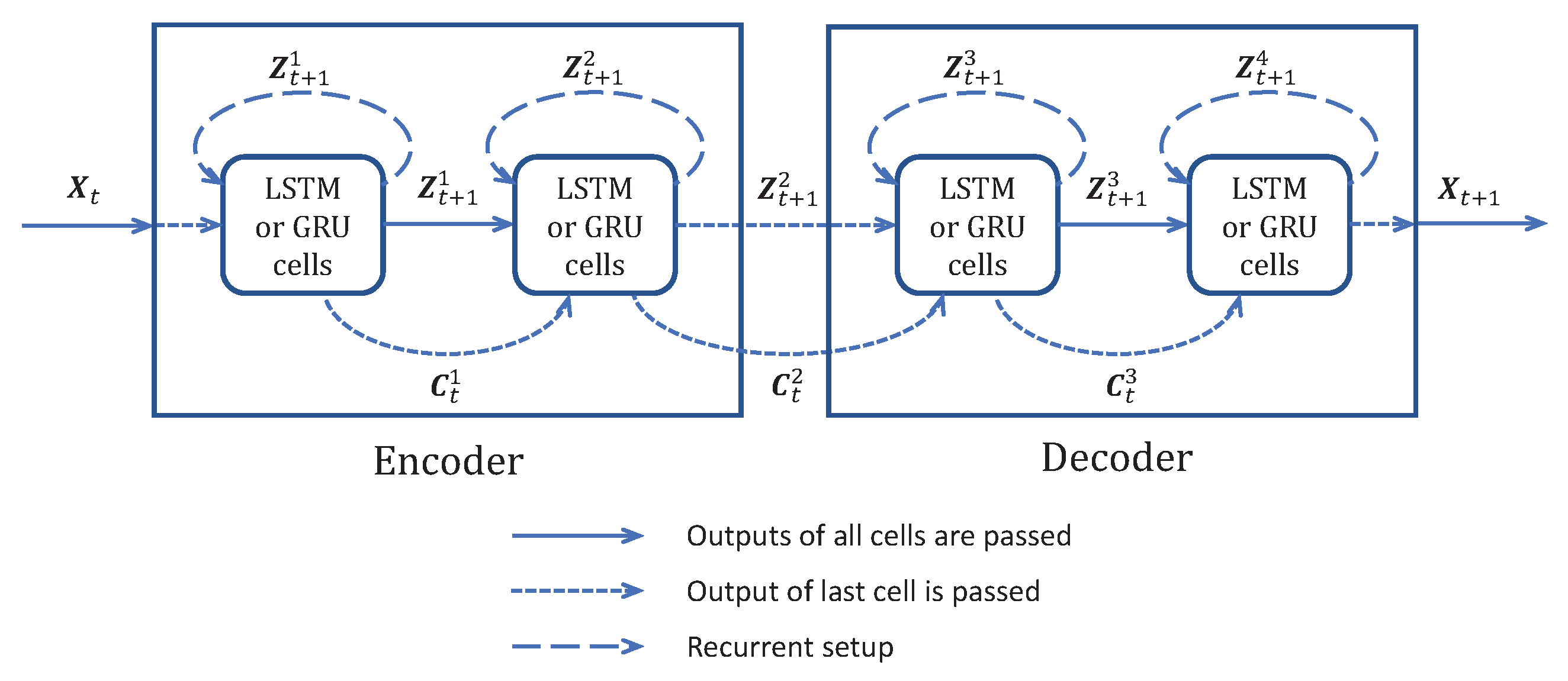
- ED-LSTM model: A version using LSTM cells with an encoder and a decoder was implemented as described in Figure 5. Because of the encoder and decoder structures, we name it ED-LSTM. This model conducts multiple step-ahead forecasts and can forecast from . The model incorporates LSTM cells organized into four layers: two layers of encoding into a bottleneck and two layers of decoding from the bottleneck. The first encoding layer is composed of 100 spatial units looped 180 times on the prior IRIS data and all of the cell outputs are returned by the model using TensorFlow option , returning a spatiotemporal output accounting for a spatial compression. The second encoding layer is composed of 100 spatial units looped 180 times and only the last cell outputs of the recurrences are returned, returning a 100-dimensional bottleneck that accounts for a spatial compression followed by a temporal compression. This bottleneck representation is repeated 60 times for IRIS data in order to model the decoding of 60 posterior time steps to forecast. After this repetition, the data are and fed to the first decoding layer with 100 spatial units looped 60 times and initialized with the states obtained from the second encoding layer; indeed, the structure is symmetrical, such that the first and second decoding layers are, respectively, the images of the second and the first encoding layers. All cell outputs are returned by the model using TensorFlow option , such that a spatiotemporal output is returned. The second layer of the decoder is designed with 100 spatial units looped 60 times and initialized with the states obtained from the first encoding layer, such that a output is returned. In the end, a time-distributed dense layer is used to map the output data into a MTS data format. For these models, the input and output shapes are determined by the data and one can only change the number of spatial cells and used, respectively, in the first and second layers of the encoding part. determines the dimension of the bottleneck and on the IRIS data, . Our experiments show that the results of these models do not depend much on the values of and , but significantly drop when is very small, close to 1. Details of the architecture are given in the Appendix B, Table A4.
- ED-GRU model: This model follows the same structure as the ED-LSTM but with GRU cells instead of LSTM cells. The structure and number of units are the same as with ED-LSTM models, but GRU cells are used instead of LSTM ones. Details of the architecture are given in the Appendix B, Table A4.
- NBeats model: We use the code given in the original paper [3]. This model can forecast from . The model is used in its generic architecture as described in [3], with 2 blocks per stack, theta dimensions of , shared weights in stacks, and 100 hidden layers units. For IRIS data, the prior is , the forecast posterior is , and the backcast posterior is , but we also use a skipping layer to connect the input to the backcast posterior, such that the model is forced to learn the transition between the prior and the forecast posterior. we attempted NBeats with other settings and other numbers of stacks without the gain of performance, and when the number of stacks became greater than 4, the model failed to initialize on our machines.
3. Results
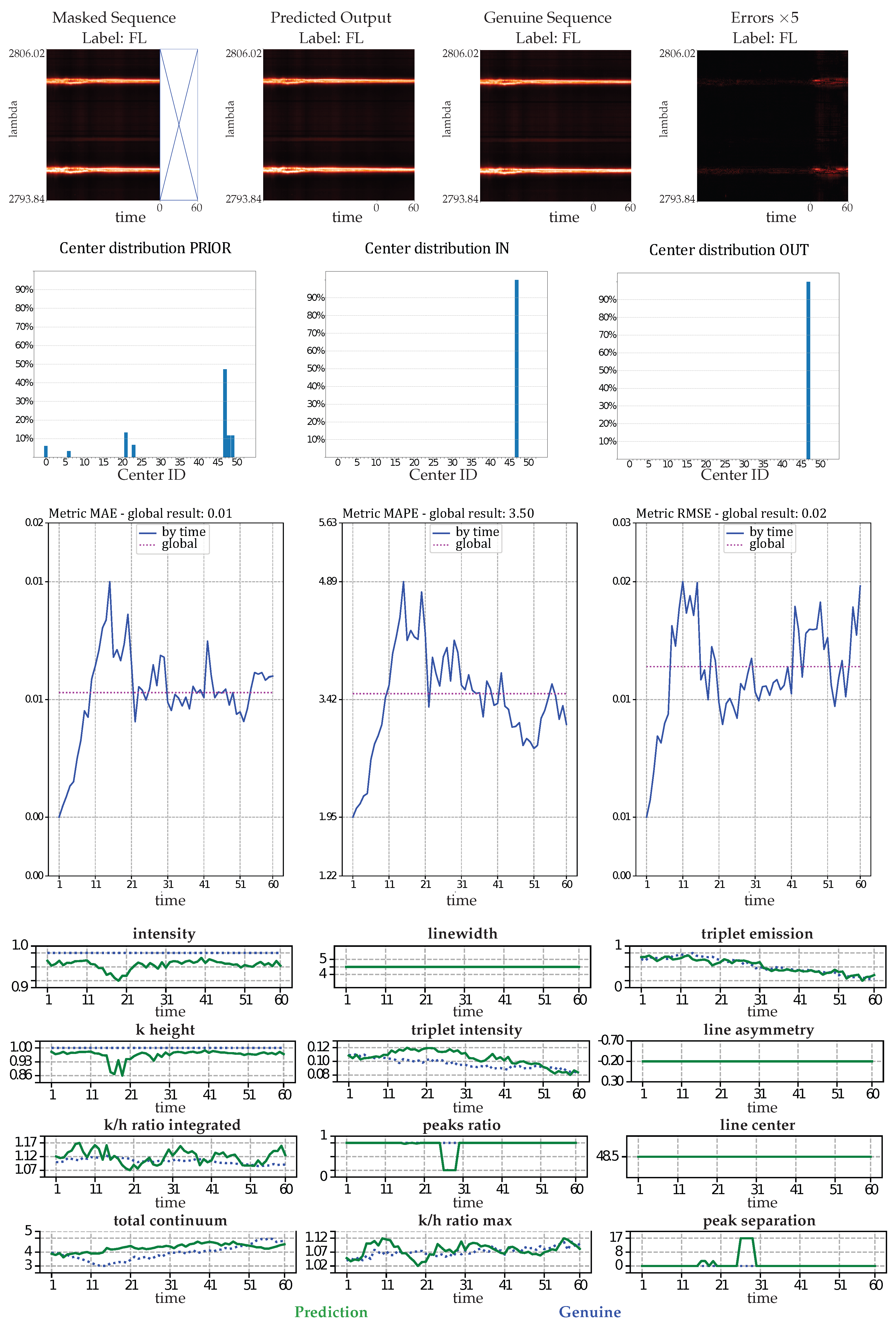
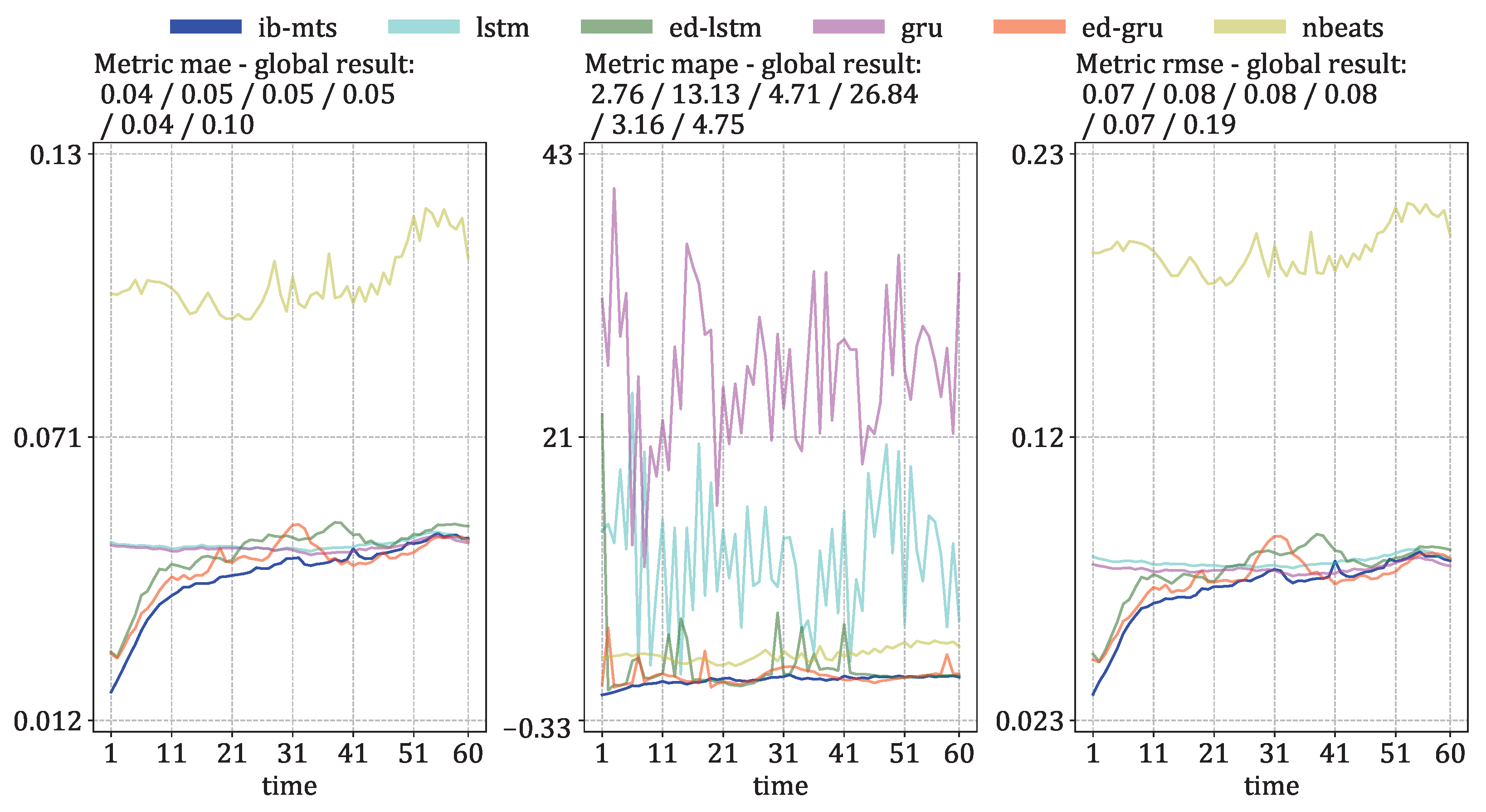
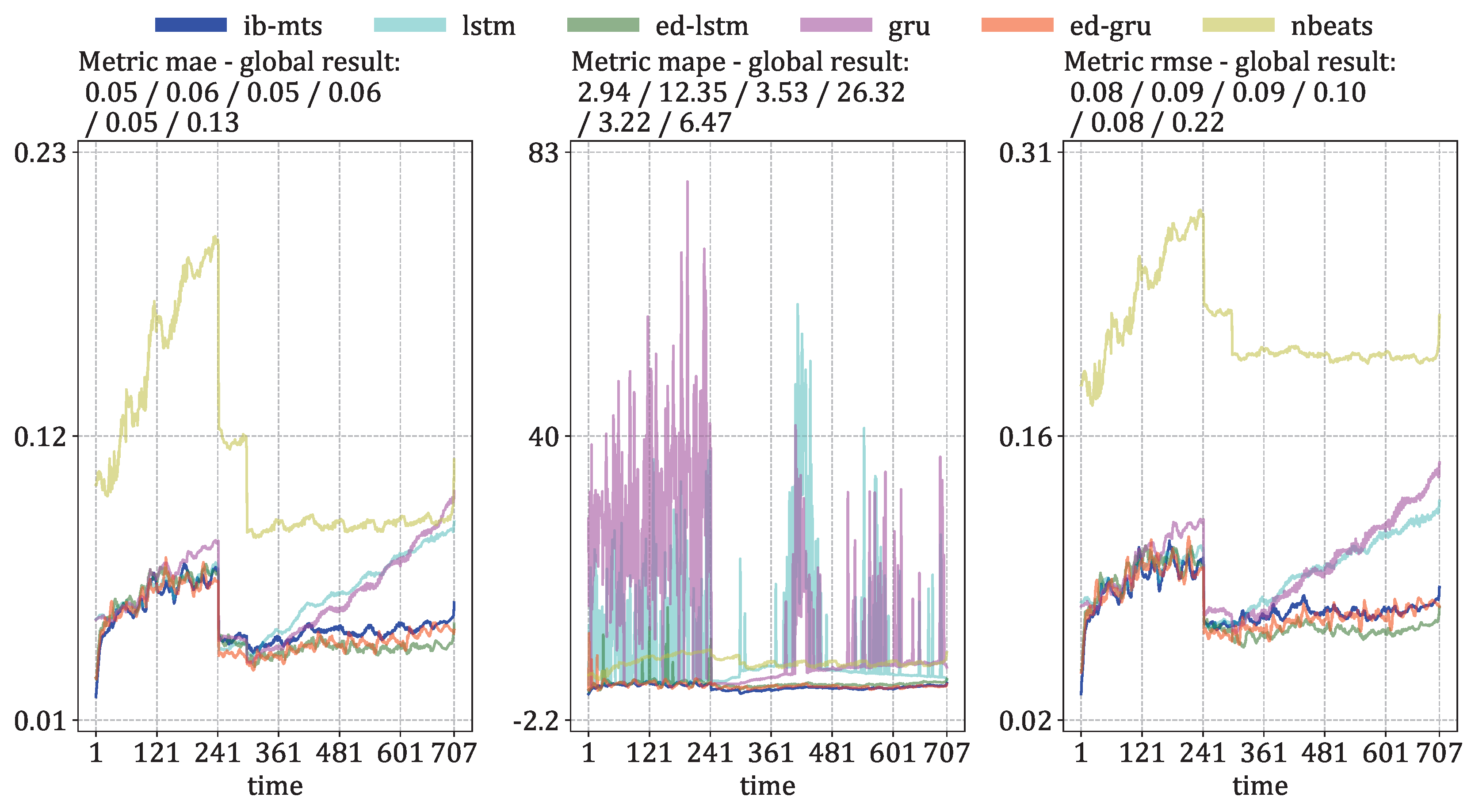
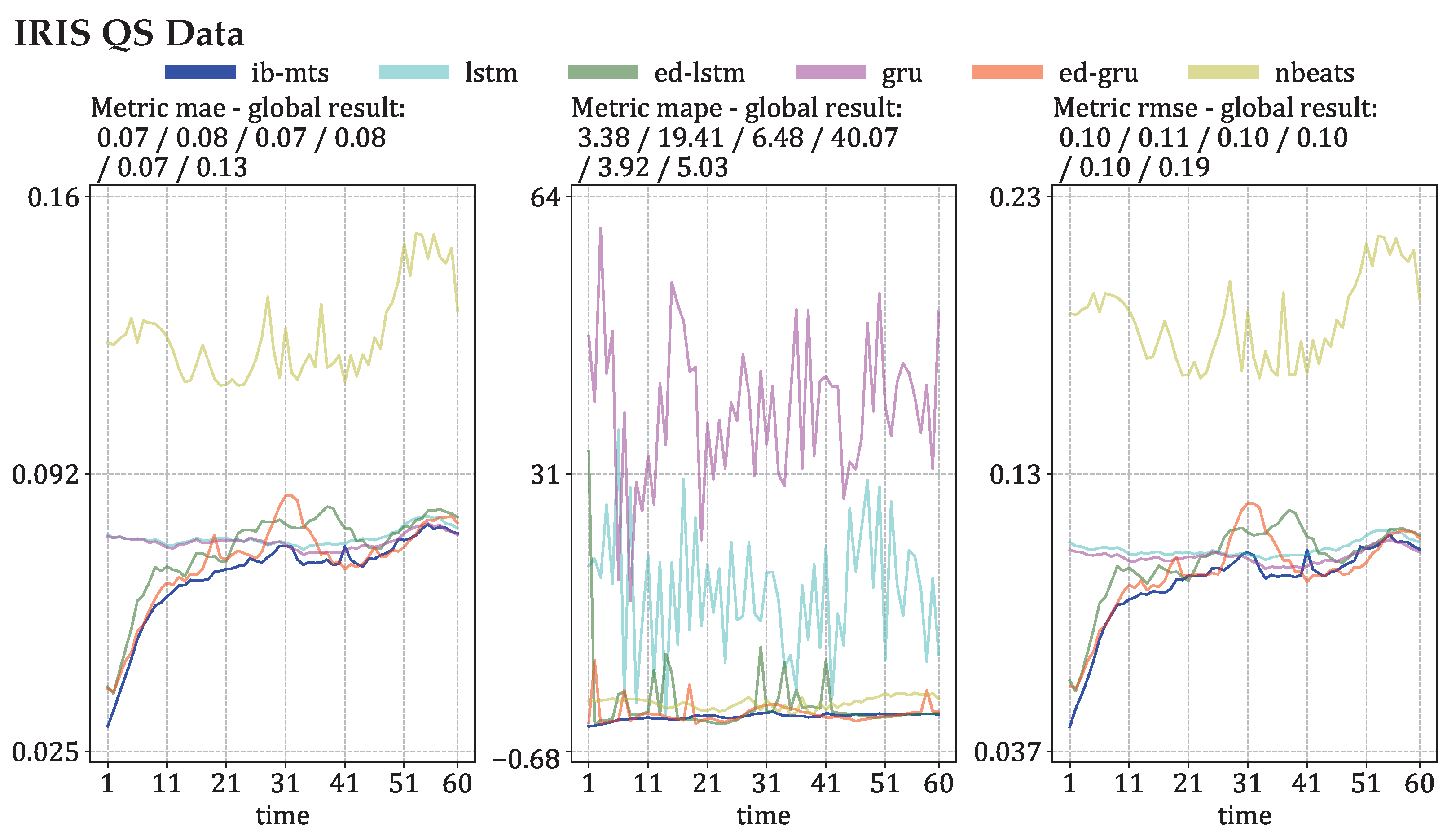
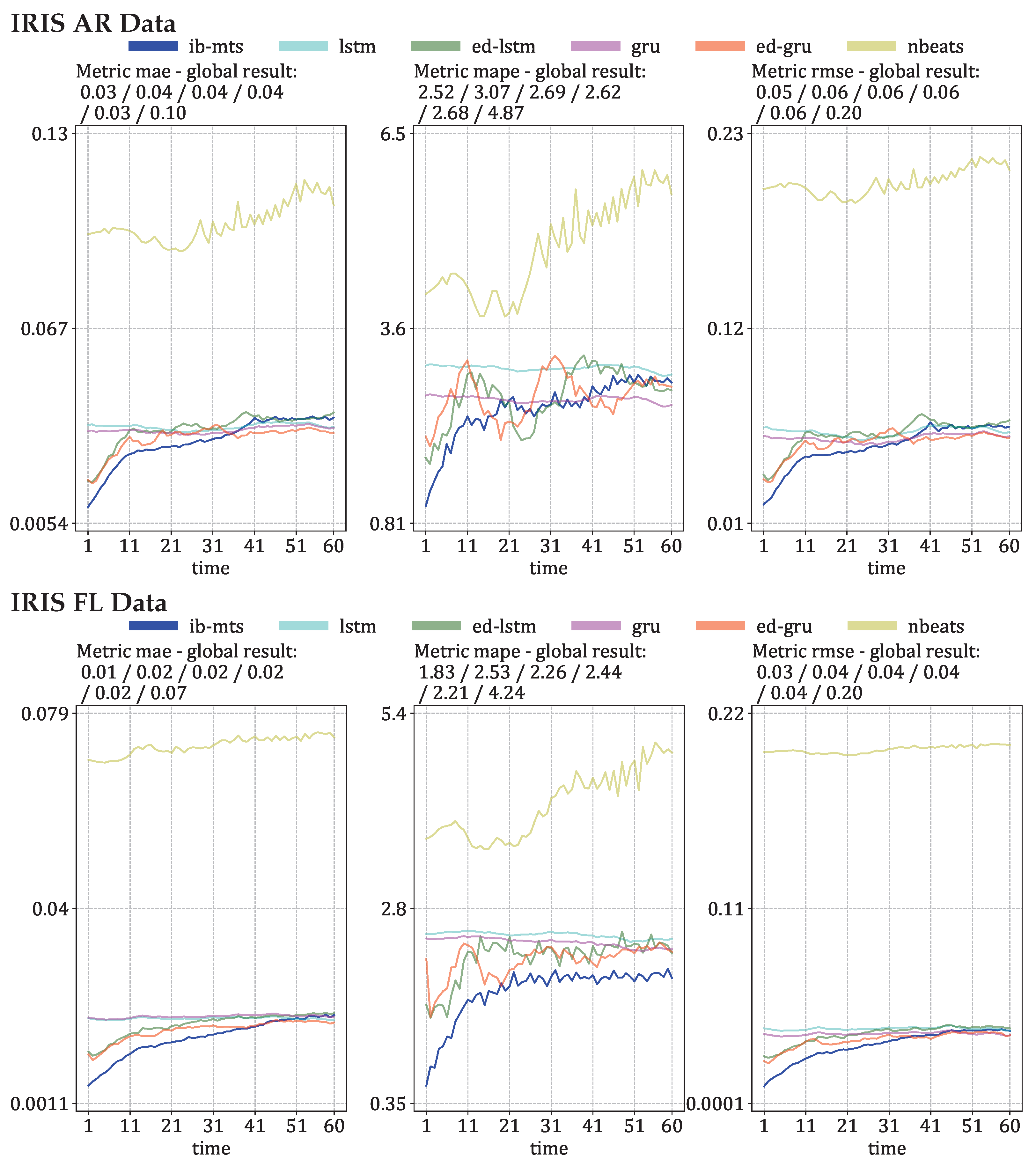
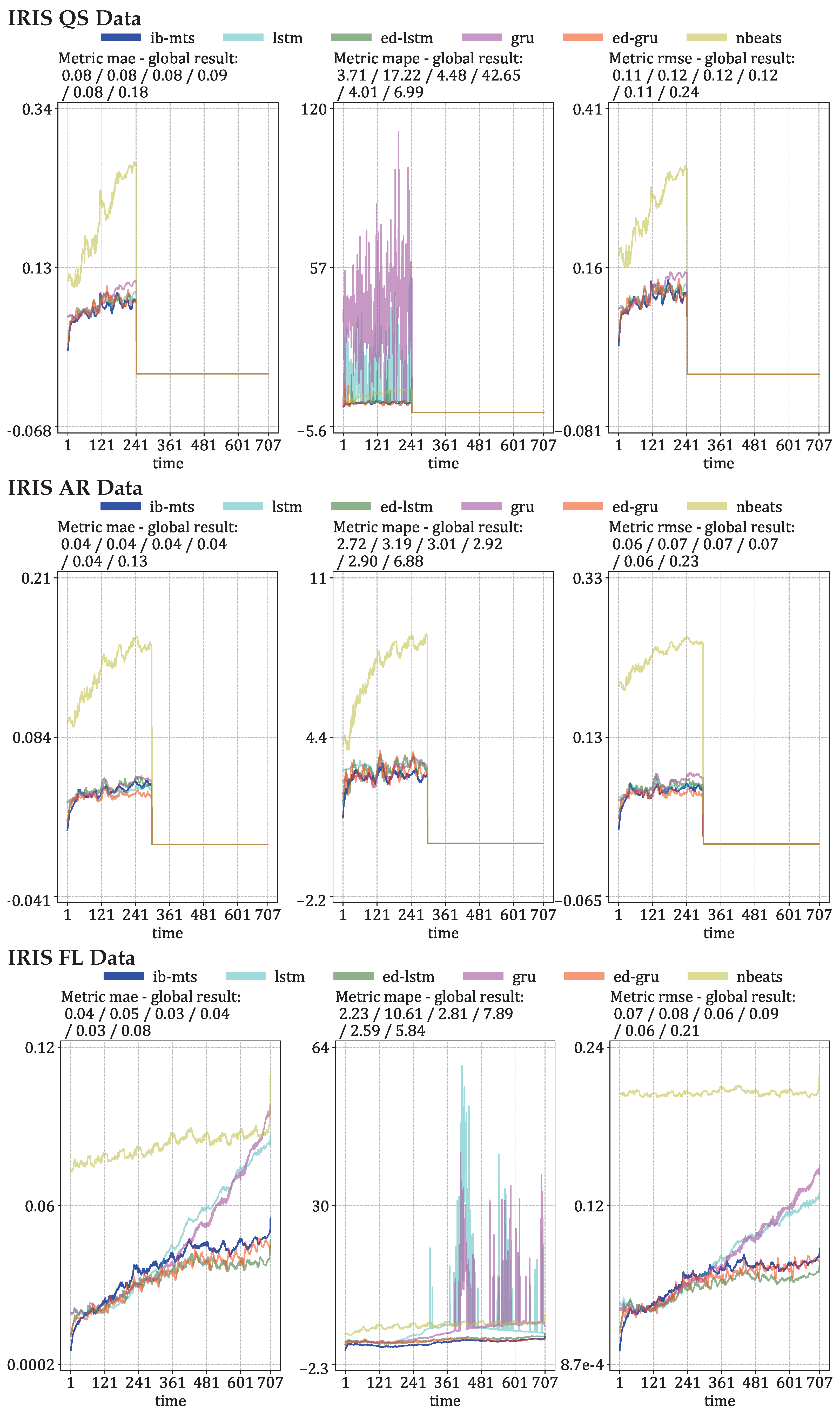
- MTS metrics: MAE, MAPE, and RMSE evaluation. These metrics are defined at each time step as the means of for MAE, for MAPE, and the square root of the mean of for RMSE.
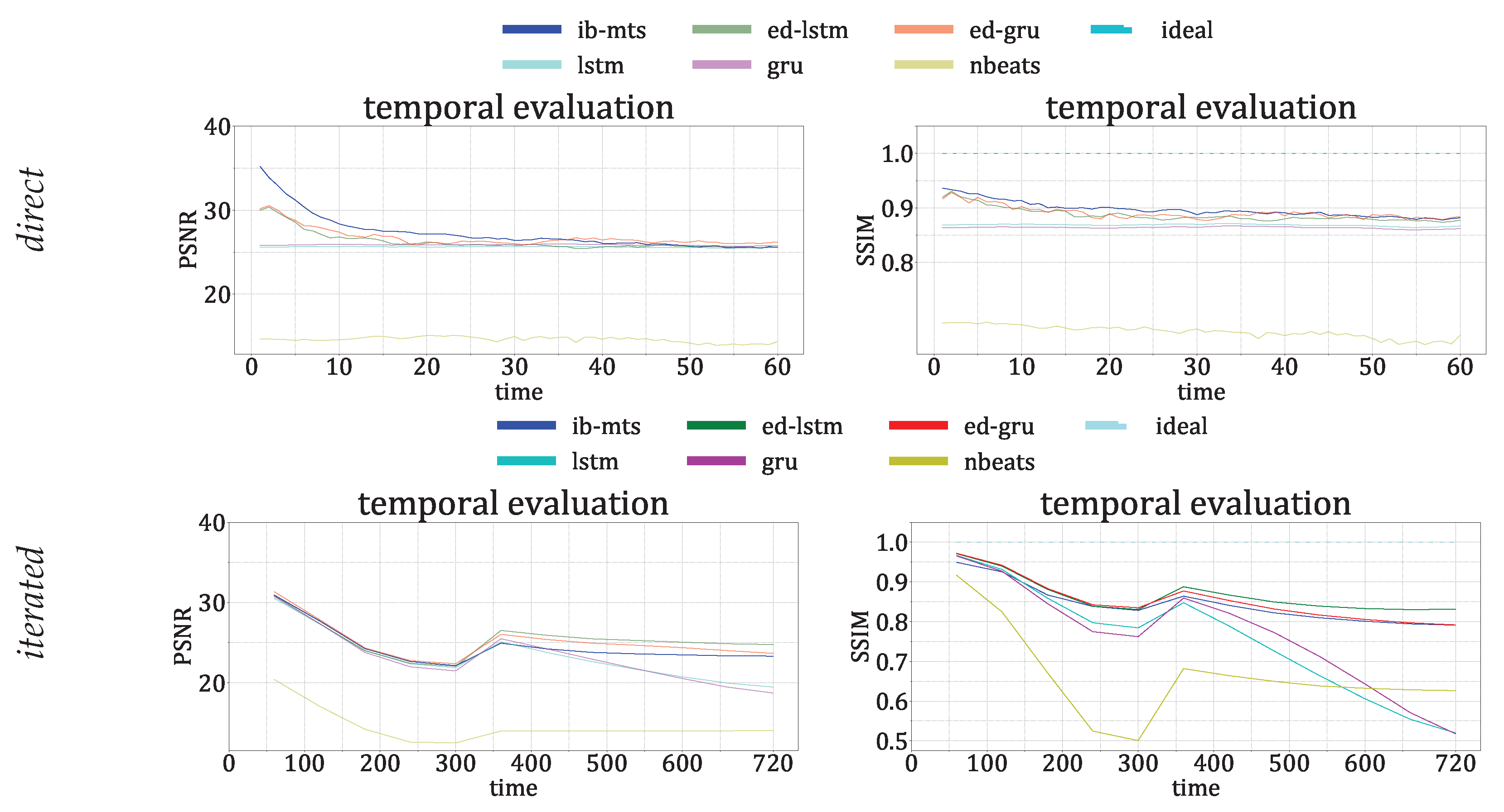
- CV metrics: PSNR and SSIM evaluation. The is defined at each time step t as , with being the mean of . The larger the PSNR, the better the prediction. The SSIM is defined at each time step by [84]:where L is the dynamic range of the pixel values, usually ; and are the mean and standard deviations of all possible windows of length 7 in the time step data , which are similar for and for the predicted time step data . is the covariance between all corresponding windows of length 7 on and . The SSIM has a maximum of 1 when and quantifies the visual structure present in the one-dimensional graph [84].
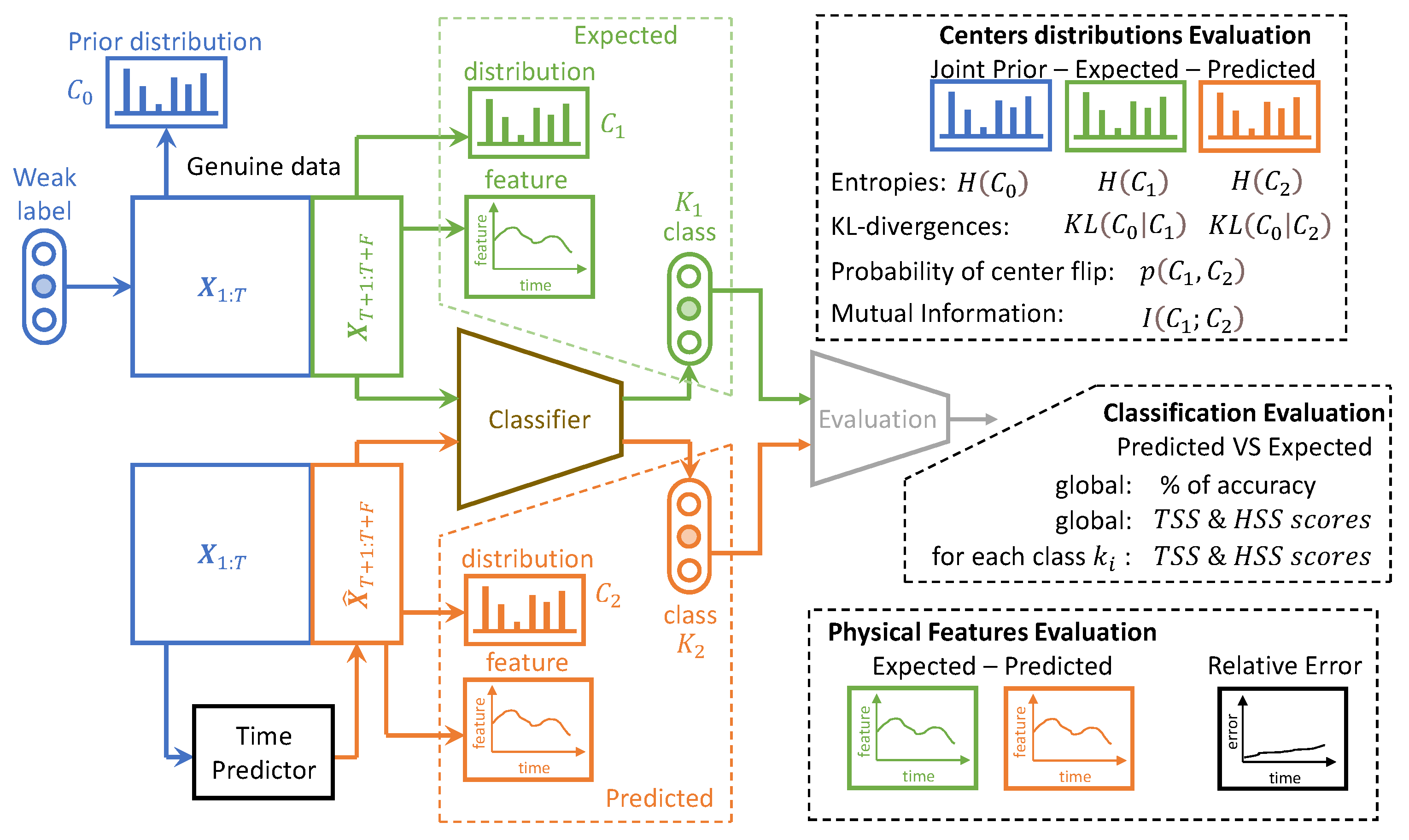
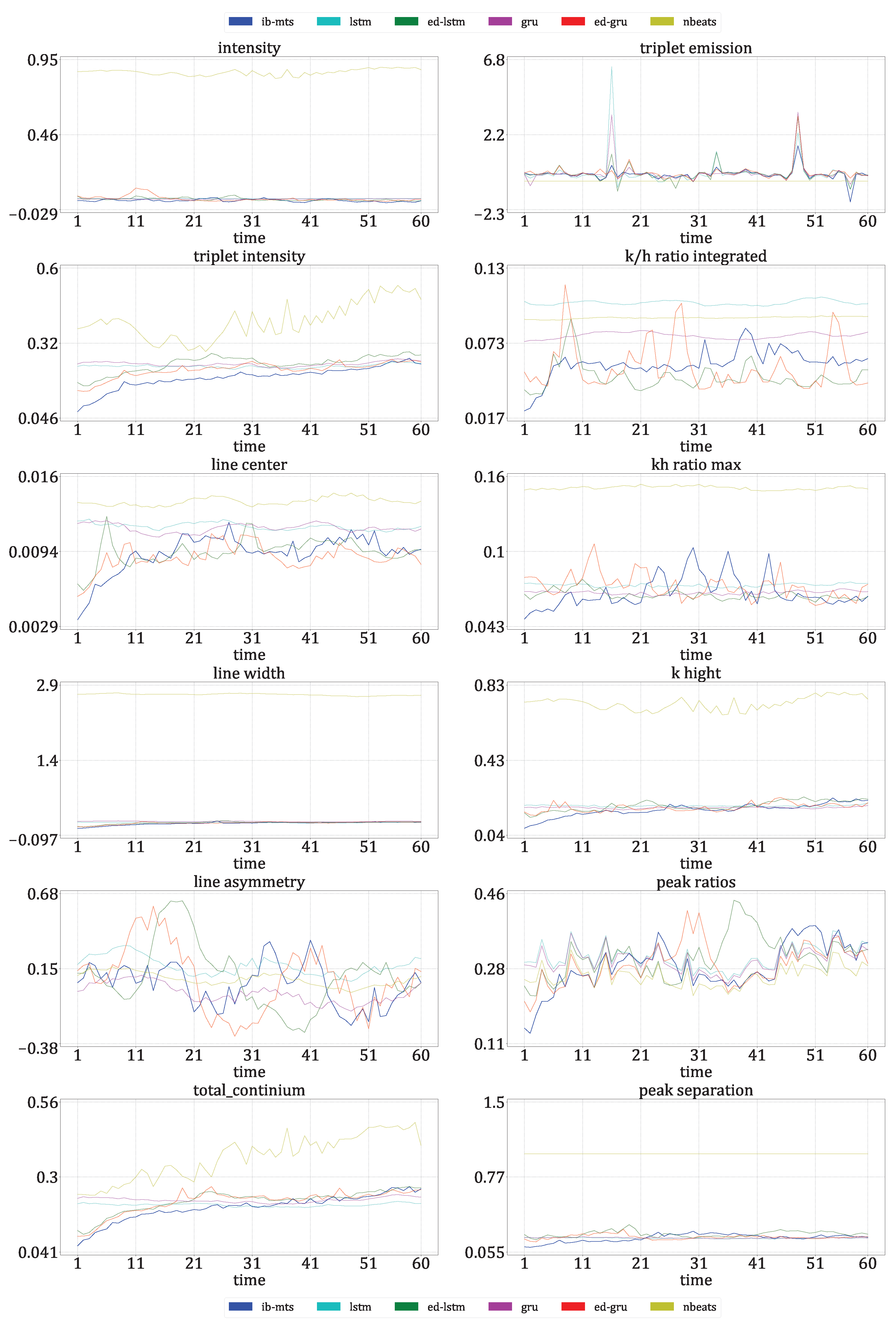
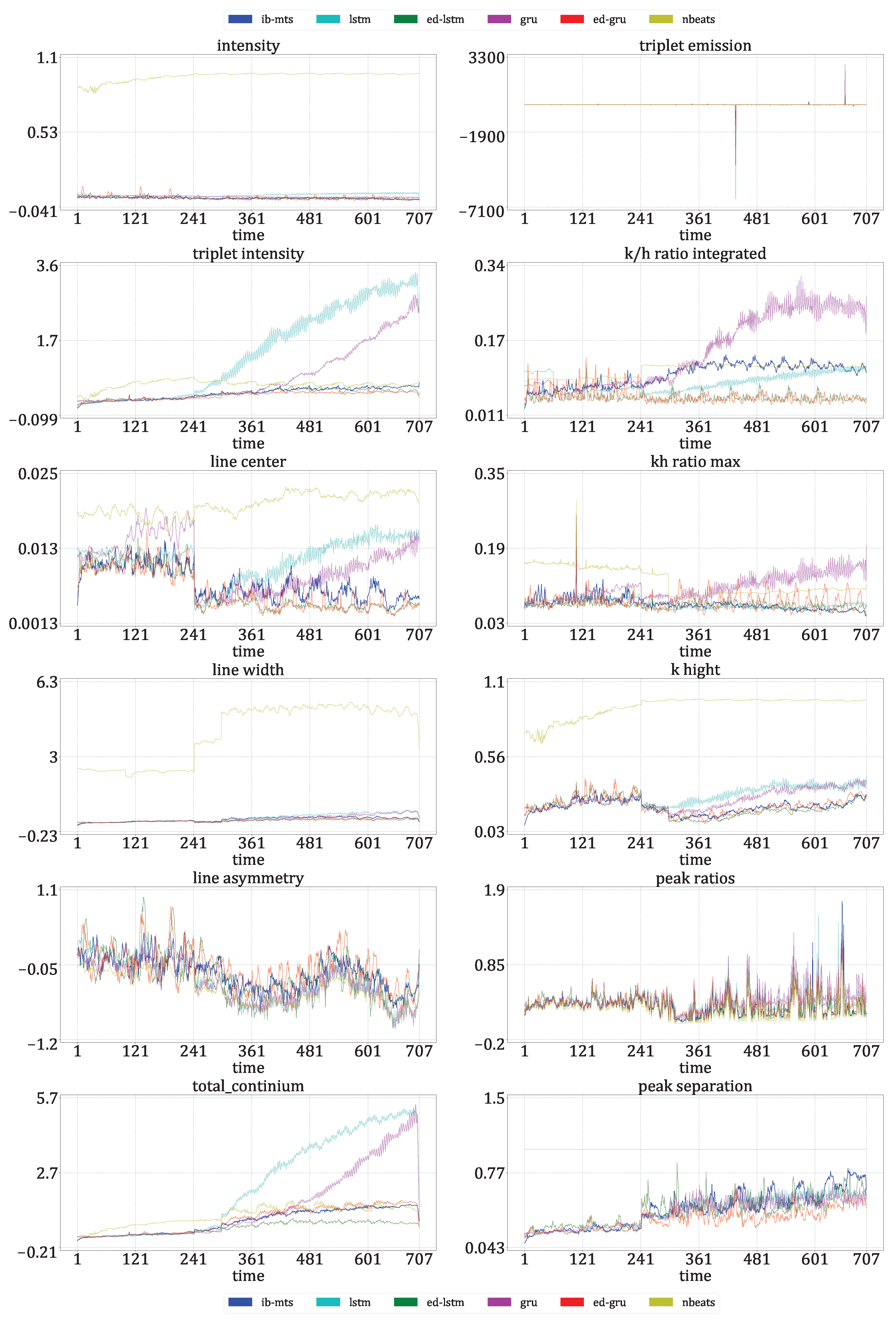
- Astrophysical features evaluation: Twelve features defined in [72] are evaluated for IRIS data. For these data, each time step corresponds to an observed spectral line in a particular region of the Sun. The intensity, triplet intensity, line center, line width, line asymmetry, total continuum, triplet emission, k/h ratio integrated, k/h ratio max, k-height, peak ratio, and peak separation are the twelve measures on these spectral lines. These features provide insight into the nature of physics occurring at the observed region of the Sun. These metrics are evaluated at each time to show that the IB principle and a powerful CV metric are sufficient to provide reliable predictions in terms of physics.
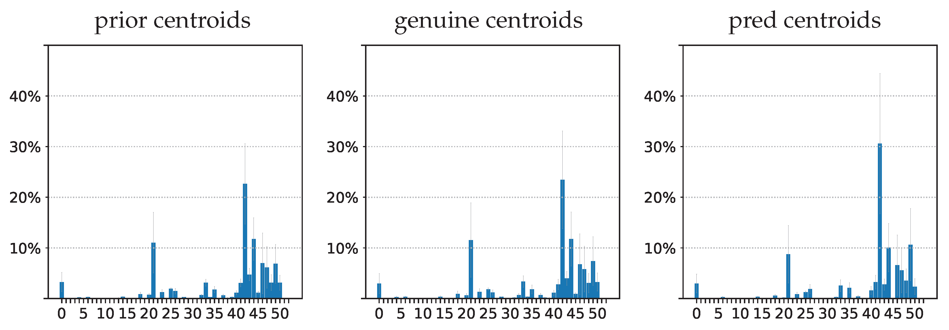
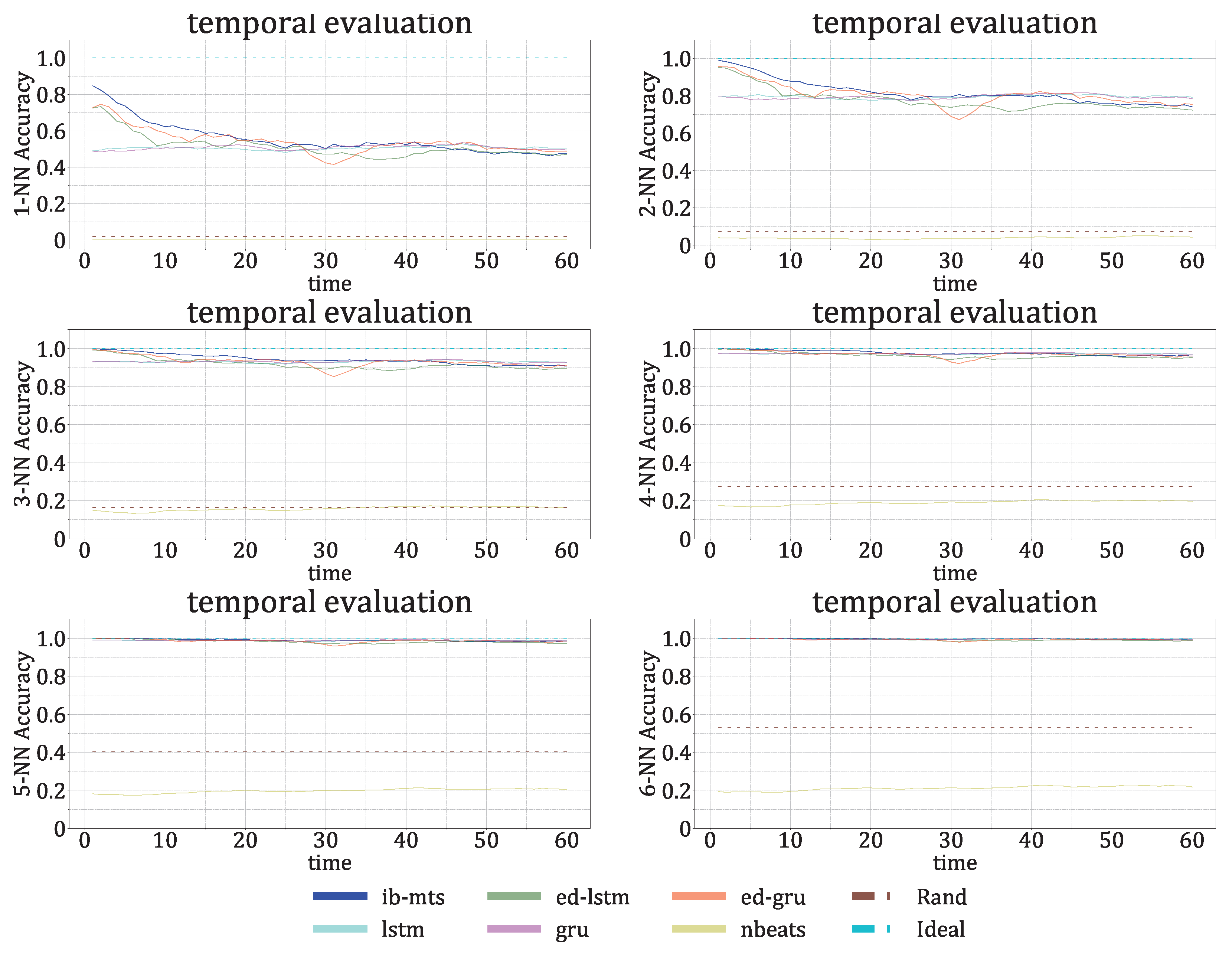
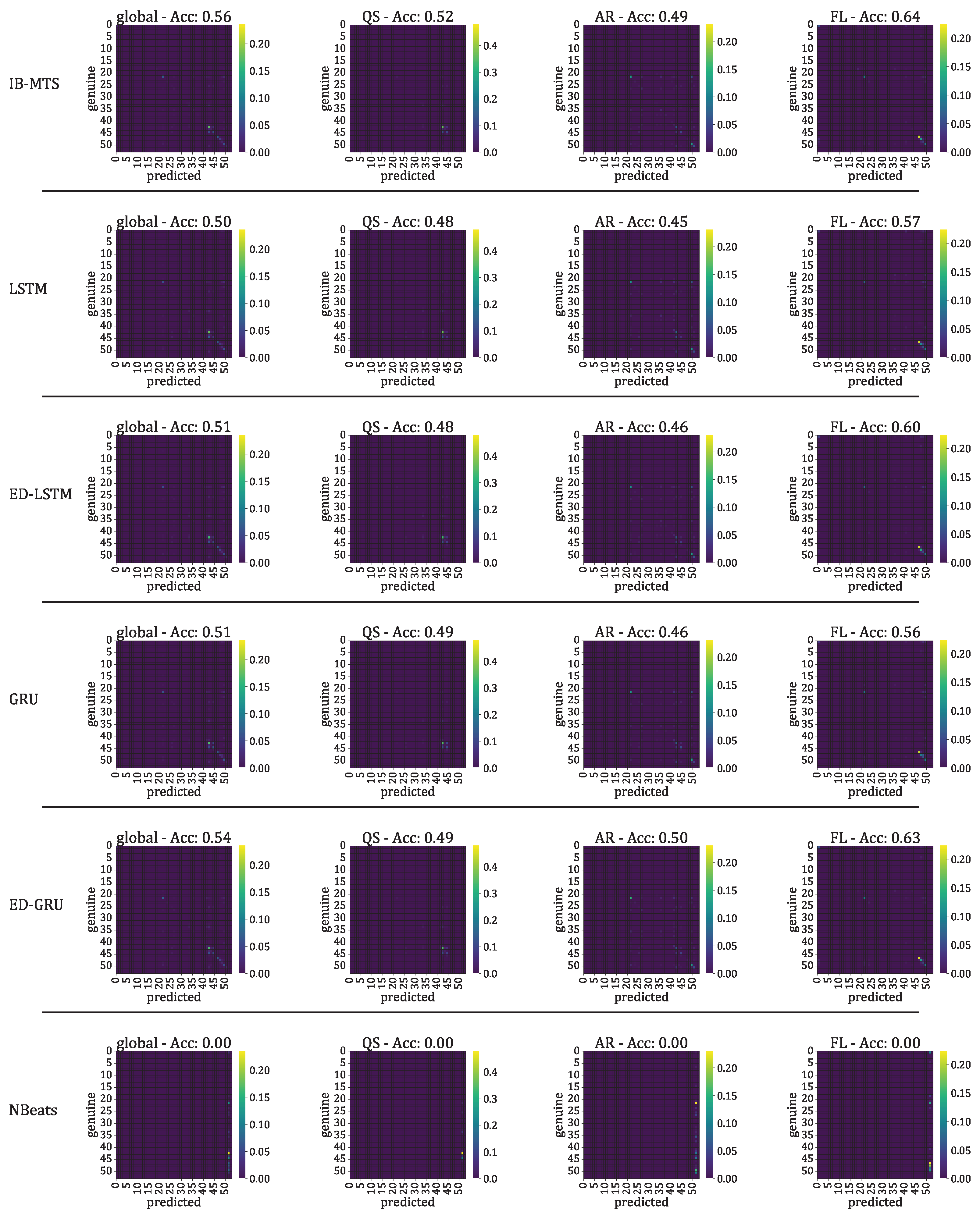
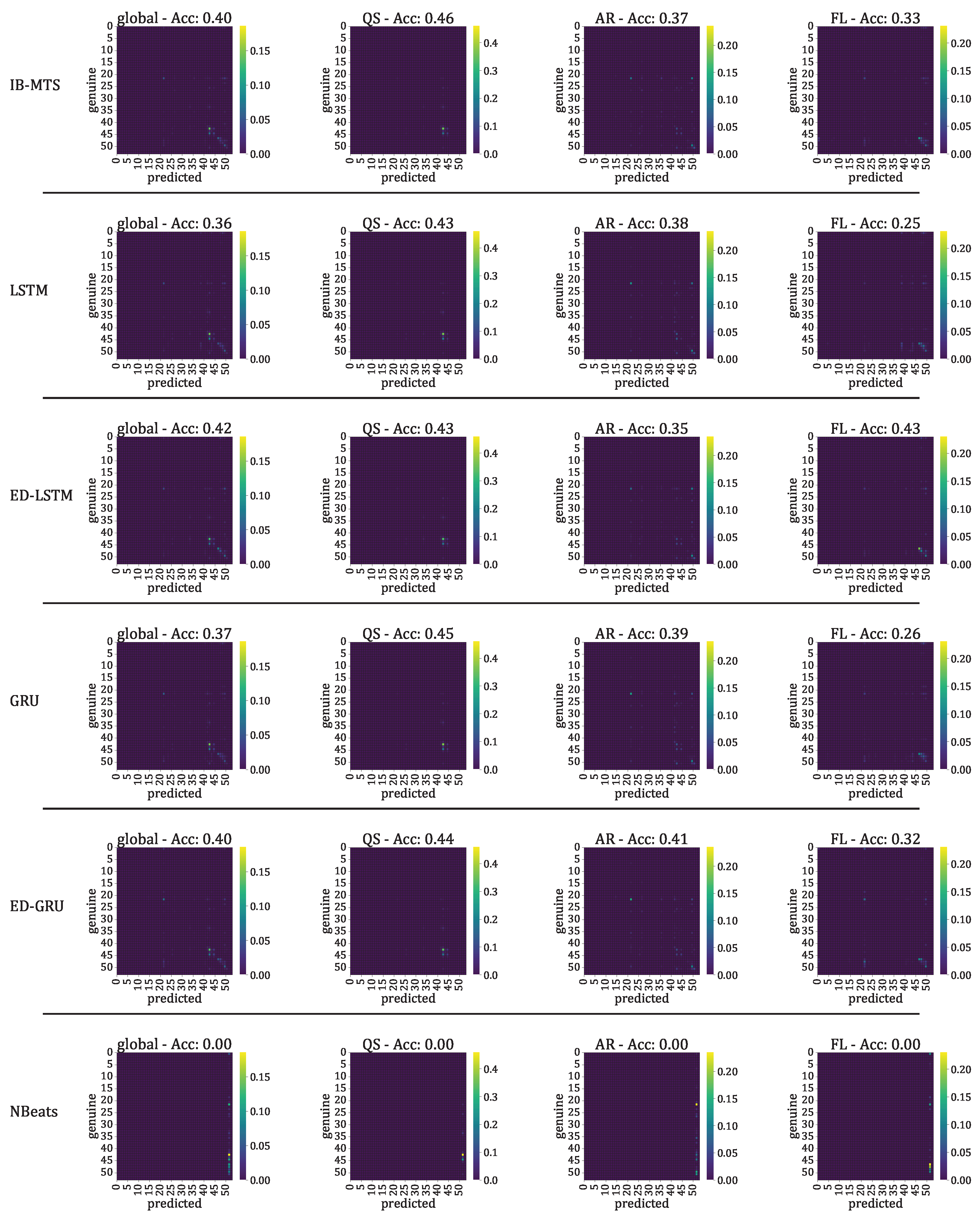
- The IB evaluation is performed on centroid distributions in the prior , genuine , and predicted forecasts . A k-means was performed in [55] for the spectral lines that are to be predicted over time. The corresponding centroids C are used in this work to evaluate information theory measurements on the quantized data. Entropies for the prior , genuine , and predicted distributions were averaged on the test data, and a comparison of the distributions between the prediction and the genuine was evaluated by computing the mutual information .
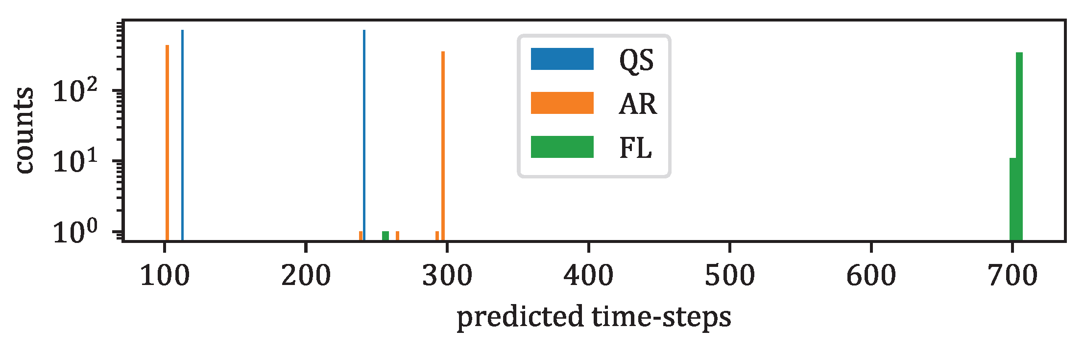
- The classification accuracy between the genuine and the forecast classifications was also evaluated. In the context of the IRIS data, three classes of solar activity are considered: QS, AR, and FL. Classifications are compared between the genuine target and predicted forecast , to assert whether the forecast activity complies with the targeted activity. [76] and [77] are evaluated globally and for each prediction class. These scores are defined in Section 2.8.
3.1. Evaluations of Predictions on IRIS Data
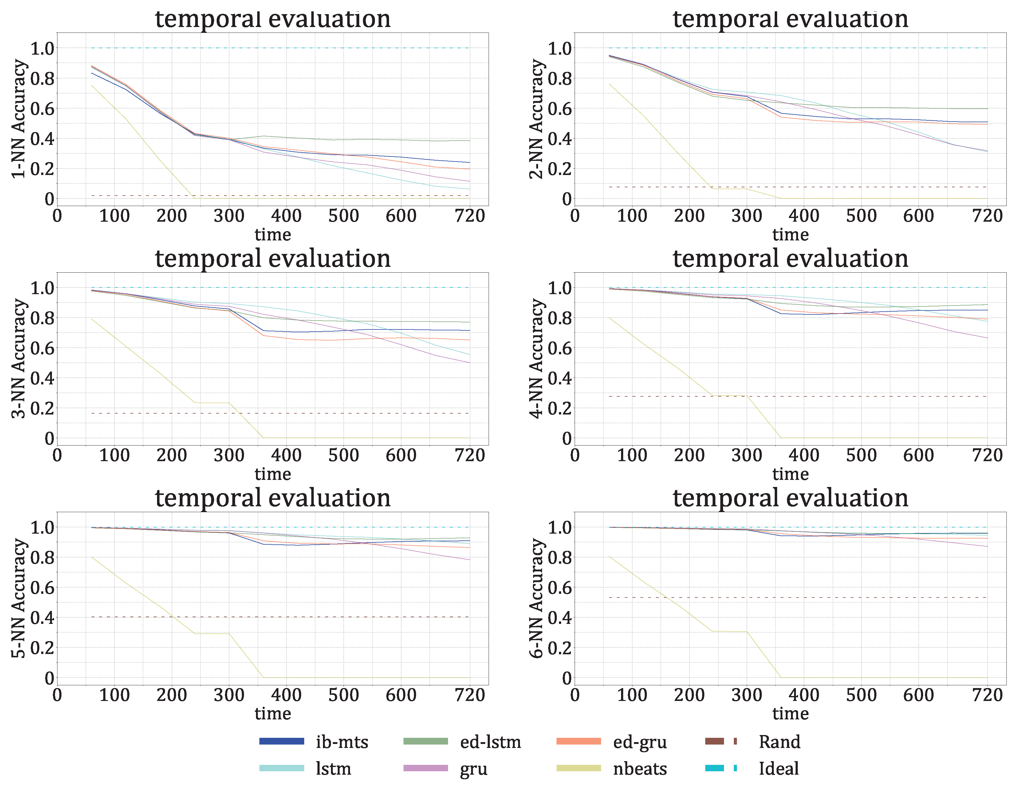
Longer Predictions
3.2. MTS Metrics Evaluation
3.3. Computer Vision Metrics Evaluation
3.3.1. Information Bottleneck Evaluation on IRIS Data
3.3.2. Astrophysical Evaluations
3.3.3. Solar Activity Classification
4. Discussion
4.1. Conclusions
4.2. Spatial Sorting of MTS Data
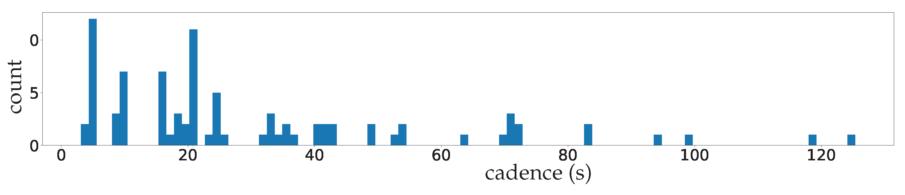
4.3. Non-Homogeneous Cadences of IRIS Data
4.4. Pros
4.5. Cons and Possible Extensions
4.6. Future Research Directions
Author Contributions
Funding
Institutional Review Board Statement
Data Availability Statement
Acknowledgments
Conflicts of Interest
Abbreviations
| AL | solar power dataset for the year 2006 in Alabama |
| AR | solar active region |
| ARIMA | autoregressive integrated moving average model |
| CV | computer vision |
| DNN | deep neural network |
| FL | solar flare |
| GNN | graph neural network |
| GRU | gated recurrent unit |
| HSS | Heidke skill score |
| IB | information bottleneck |
| IRIS | NASA’s interface region imaging spectrograph satellite |
| IT | information theory |
| LSTM | long short-term memory model |
| MAE | mean absolute error |
| MAPE | mean absolute percentage error |
| ML | machine learning |
| MOS | mean opinion score |
| MSE | mean square error |
| MTS | multiple time series |
| NLP | natural language processing |
| NN | neural network |
| PB | PeMS-BAY dataset |
| PC | partial convolution |
| PSNR | peak signal-to-noise ratio |
| QS | quiet Sun |
| RAM | random access memory |
| RGB | red–green–blue |
| RMSE | root mean square error |
| RNN | recurrent neural network |
| SSIM | structural similarity |
| TS | time series |
| TSS | true skill statistic |
Appendix A. Theory

| Random Variables | |
|---|---|
| generic spatiotemporal data | |
| estimation of | |
| T | scalar duration of the prior sequence |
| F | scalar duration of the posterior sequence |
| M | spatial size of spatiotemporal data |
| multidimensional data at time step t | |
| scalar value at time step t and spatial index m | |
| prior sequence | |
| prior sequence estimation | |
| posterior genuine sequence | |
| posterior genuine sequence estimation | |
| full sequence | |
| full sequence estimation | |
| bottleneck | |
| transition from prior to posterior | |
| IB bottleneck for transition learning | |
| IB bottleneck of AE | |
| generic mask for spatiotemporal data | |
| prior mask | |
| posterior mask | |
| full mask | |
| mask at the IB bottleneck for transition | |
| learning | |
| & & | vectors and matrices of ones, eventually |
| with specified length or and sizes. | |
| & & | vectors and matrices of zeros, eventually |
| with specified length or and sizes. | |
| K & | scalar & categorical labels |
| , & | prior, genuine, and predicted centroid assignments |
| Information Theory | |
| data distribution | |
| & | (encoding/decoding) distribution with parameter (/) |
| mean by sampling from | |
| mean by sampling from | |
| & | generic entropy and cross-entropy |
| entropy parametrized by the encoder | |
| cross-entropy parametrized by the encoder and the decoder | |
| & | -divergence & mutual information |
| & | Encoding and decoding mutual information |
| Layers & mappers | |
| Identity mapper | |
| Concatenation of tensors | |
| (-/Binary/Partial) Convolutional layer | |
| (-/Binary/Partial) Deconvolutional layer | |
| Losses & metrics | |
| generic loss | |
| upper bound on the loss | |
| with Laplacian assumption of | |
| for a U-Net architecture | |
| relative error for feature k at time step t | |
Appendix B. Models
| Model: IB-MTS for IRIS Data | ||||
|---|---|---|---|---|
|
Layer (Type) | Output Shape | Kernel | Param # | Connected to |
| inputs_img | [(240, 240, 1)] | – | 0 | [] |
| (InputLayer) | ||||
| inputs_mask | [(240, 240, 1)] | – | 0 | [] |
| (InputLayer) | ||||
| zero_pad2d | (256, 256, 1) | – | 0 | [inputs_img] |
| (ZeroPad2D) | ||||
| zero_pad2d | (256, 256, 1) | – | 0 | [inputs_mask] |
| (ZeroPad2D) | ||||
| EncPConv2D | (128,128,64) (64, 64, 128) (32, 32, 256) (16, 16, 512) (8, 8, 512) (4, 4, 512) (2, 2, 512) (1, 1, 512) |
7 5 5 3 3 3 3 3 |
18880 410240 1639168 2361856 4721152 4721152 4721152 4721152 | [EncReLu, |
| (PConv2D) | EncPConv2D[1]] | |||
| EncBN | [EncPConv2D[0]] | |||
| (BatchNorm) | ||||
| EncReLu | [EncBN] | |||
| (Activation) | ||||
| DecUpImg | (2, 2, 512) (4, 4, 512) (16, 16, 512) (32, 32, 512) (64, 64, 256) (128, 128, 128) (256, 256, 64) (256, 256, 3) |
3 3 3 3 3 3 3 3 |
9439744 9439744 9439744 9439744 3540224 885376 221504 3621 | [DecLReLU] |
| (UpSampling2D) | ||||
| DecUpMsk | [DecPConv2D[1]] | |||
| (UpSampling2D) | ||||
| DecConcatImg | [EncReLu, | |||
| (Concatenate) | DecUpImg] | |||
| DecConcatMsk | [EncPConv2D[1], | |||
| (Concatenate) | DecUpMsk] | |||
| DecPConv2D | [DecConcatImg, | |||
| (PConv2D) | DecConcatMsk] | |||
| DecBN | [DecPConv2D[0]] | |||
| (BatchNorm) | ||||
| DecLReLU | [DecBN] | |||
| (LeakyReLU) | ||||
| outputs_img | (256, 256, 1) | 1 | 4 | [DecLReLU7] |
| (Conv2D) | ||||
| OutCrop | (240, 240, 1) | – | 0 | [outputs_img] |
| (Cropping2D) | ||||
| Total params: 65,724,969 | ||||
| Model: LSTM for IRIS Data | ||||
|---|---|---|---|---|
| Layer (Type) | Output Shape | Units | Param # | Connected to |
| inputs_seq (InputLayer) | [(240, 240)] | – | 0 | [] |
| slice (SlicingOp) | (180, 240) | – | 0 | [inputs_seq] |
| lstm (LSTM) | (180, 240) | 240 | 461760 | [slice] |
| slice (SlicingOp) | (60, 240) | – | 0 | [lstm] |
| concat (TFOp) | (240, 240) | – | 0 | [slice, slice] |
| Total params: 461,760 | ||||
| Model: ED-LSTM for IRIS Data | ||||
|---|---|---|---|---|
| Layer (Type) | Output Shape | Units | Param # | Connected to |
| inputs_seq (InputLayer) | [(240, 240)] | – | 0 | [] |
| slice (SlicingOp) | (180, 240) | – | 0 | [inputs_seq] |
| lstm (LSTM) | [(180, 100), (100)] | 100 | 136400 | [slice] |
| lstm (LSTM) | [(100), (100)] | 100 | 80400 | [lstm[0]] |
| repeat_vector (RepeatVector) | (60, 100) | – | 0 | [lstm[0]] |
| lstm (LSTM) | (60, 100) | 100 | 80400 | [repeat_vector, lstm[0][2]] |
| lstm (LSTM) | (60, 100) | 100 | 80400 | [lstm[0], lstm[1]] |
| time_distributed (TimeDistributed) | (60, 240) | 240 | 24240 | [lstm] |
| concat (TFOp) | (240, 240) | – | 0 | [slice, time_distributed] |
| Total params: 401,840 | ||||
Appendix C. Results


References
- Gangopadhyay, T.; Tan, S.Y.; Jiang, Z.; Meng, R.; Sarkar, S. Spatiotemporal Attention for Multivariate Time Series Prediction and Interpretation. arXiv 2020, arXiv:2008.04882. [Google Scholar]
- Flunkert, V.; Salinas, D.; Gasthaus, J. DeepAR: Probabilistic Forecasting with Autoregressive Recurrent Networks. arXiv 2017, arXiv:1704.04110. [Google Scholar]
- Oreshkin, B.N.; Carpov, D.; Chapados, N.; Bengio, Y. N-BEATS: Neural basis expansion analysis for interpretable time series forecasting. arXiv 2019, arXiv:1905.10437. [Google Scholar]
- Liu, G.; Reda, F.A.; Shih, K.J.; Wang, T.; Tao, A.; Catanzaro, B. Image Inpainting for Irregular Holes Using Partial Convolutions. arXiv 2018, arXiv:1804.07723. [Google Scholar]
- Rumelhart, D.E.; McClelland, J.L. Learning Internal Representations by Error Propagation. In Parallel Distributed Processing: Explorations in the Microstructure of Cognition: Foundations; The MIT Press: Cambridge, MA, USA, 1987; Volume 1, pp. 318–362. [Google Scholar]
- Hochreiter, S.; Schmidhuber, J. Long Short-Term Memory. Neural Comput. 1997, 9, 1735–1780. [Google Scholar] [CrossRef]
- Dobson, A. The Oxford Dictionary of Statistical Terms; Oxford University Press: Oxford, UK, 2003; p. 506. [Google Scholar]
- Kendall, M. Time Series; Charles Griffin and Co Ltd.: London, UK; High Wycombe, UK, 1976. [Google Scholar]
- West, M. Time Series Decomposition. Biometrika 1997, 84, 489–494. [Google Scholar] [CrossRef]
- Sheather, S. A Modern Approach to Regression with R; Springer: New York, NY, USA, 2009. [Google Scholar] [CrossRef]
- Molugaram, K.; Rao, G.S. Chapter 12—Analysis of Time Series. In Statistical Techniques for Transportation Engineering; Molugaram, K., Rao, G.S., Eds.; Butterworth-Heinemann: Oxford, UK, 2017; pp. 463–489. [Google Scholar] [CrossRef]
- Gardner, E.S. Exponential smoothing: The state of the art. J. Forecast. 1985, 4, 1–28. [Google Scholar] [CrossRef]
- Box, G.; Jenkins, G.M. Time Series Analysis: Forecasting and Control; Holden-Day: Cleveland, Australia, 1976. [Google Scholar]
- Curry, H.B. The method of steepest descent for nonlinear minimization problems. Quart. Appl. Math. 1944, 2, 258–261. [Google Scholar] [CrossRef]
- Cho, K.; van Merrienboer, B.; Bahdanau, D.; Bengio, Y. On the Properties of Neural Machine Translation: Encoder-Decoder Approaches. arXiv 2014, arXiv:1409.1259. [Google Scholar]
- Kazemi, S.M.; Goel, R.; Eghbali, S.; Ramanan, J.; Sahota, J.; Thakur, S.; Wu, S.; Smyth, C.; Poupart, P.; Brubaker, M. Time2Vec: Learning a Vector Representation of Time. arXiv 2019, arXiv:1907.05321. [Google Scholar] [CrossRef]
- Lim, B.; Arik, S.O.; Loeff, N.; Pfister, T. Temporal Fusion Transformers for Interpretable Multi-horizon Time Series Forecasting. arXiv 2019, arXiv:1912.09363. [Google Scholar] [CrossRef]
- Grigsby, J.; Wang, Z.; Qi, Y. Long-Range Transformers for Dynamic Spatiotemporal Forecasting. arXiv 2021, arXiv:2109.12218. [Google Scholar]
- Vaswani, A.; Shazeer, N.; Parmar, N.; Uszkoreit, J.; Jones, L.; Gomez, A.N.; Kaiser, L.; Polosukhin, I. Attention Is All You Need. arXiv 2021, arXiv:1706.03762. [Google Scholar]
- Zhou, H.; Zhang, S.; Peng, J.; Zhang, S.; Li, J.; Xiong, H.; Zhang, W. Informer: Beyond Efficient Transformer for Long Sequence Time-Series Forecasting. arXiv 2020, arXiv:2012.07436. [Google Scholar] [CrossRef]
- Scarselli, F.; Gori, M.; Tsoi, A.C.; Hagenbuchner, M.; Monfardini, G. The Graph Neural Network Model. IEEE Trans. Neural Netw. 2009, 20, 61–80. [Google Scholar] [CrossRef] [PubMed]
- Bertalmio, M.; Sapiro, G.; Caselles, V.; Ballester, C. Image Inpainting. In Proceedings of the 27th Annual Conference on Computer Graphics and Interactive Techniques, New Orleans, LA, USA, 23–28 July 2000; ACM Press/Addison-Wesley Publishing Co.: Boston, MA, USA, 2000. SIGGRAPH ’00. pp. 417–424. [Google Scholar] [CrossRef]
- Teterwak, P.; Sarna, A.; Krishnan, D.; Maschinot, A.; Belanger, D.; Liu, C.; Freeman, W.T. Boundless: Generative Adversarial Networks for Image Extension. arXiv 2019, arXiv:1908.07007 2019. [Google Scholar] [CrossRef]
- Ulyanov, D.; Vedaldi, A.; Lempitsky, V. Deep Image Prior. Int. J. Comput. Vis. 2020, 128, 1867–1888. [Google Scholar] [CrossRef]
- Dama, F.; Sinoquet, C. Time Series Analysis and Modeling to Forecast: A Survey. arXiv 2021, arXiv:2104.00164. [Google Scholar] [CrossRef]
- Tessoni, V.; Amoretti, M. Advanced statistical and machine learning methods for multi-step multivariate time series forecasting in predictive maintenance. Procedia Comput. Sci. 2022, 200, 748–757. [Google Scholar] [CrossRef]
- Lehtinen, J.; Munkberg, J.; Hasselgren, J.; Laine, S.; Karras, T.; Aittala, M.; Aila, T. Noise2Noise: Learning Image Restoration without Clean Data. arXiv 2018, arXiv:1803.04189. [Google Scholar]
- Gatys, L.A.; Ecker, A.S.; Bethge, M. Image Style Transfer Using Convolutional Neural Networks. In Proceedings of the 2016 IEEE Conference on Computer Vision and Pattern Recognition (CVPR), Las Vegas, NV, USA, 27–30 June 2016; pp. 2414–2423. [Google Scholar]
- Johnson, J.; Alahi, A.; Fei-Fei, L. Perceptual Losses for Real-Time Style Transfer and Super-Resolution. arXiv 2016, arXiv:1603.08155. [Google Scholar]
- Ledig, C.; Theis, L.; Huszar, F.; Caballero, J.; Cunningham, A.; Acosta, A.; Aitken, A.; Tejani, A.; Totz, J.; Wang, Z.; et al. Photo-Realistic Single Image Super-Resolution Using a Generative Adversarial Network. arXiv 2016, arXiv:1609.04802. [Google Scholar]
- Ronneberger, O.; Fischer, P.; Brox, T. U-Net: Convolutional Networks for Biomedical Image Segmentation. arXiv 2015, arXiv:1505.04597. [Google Scholar]
- Kramer, M.A. Nonlinear principal component analysis using autoassociative neural networks. AIChE J. 1991, 37, 233–243. [Google Scholar] [CrossRef]
- Tishby, N.; Zaslavsky, N. Deep Learning and the Information Bottleneck Principle. arXiv 2015, arXiv:1503.02406. [Google Scholar] [CrossRef]
- Costa, J.; Costa, A.; Kenda, K.; Costa, J.P. Entropy for Time Series Forecasting. In Proceedings of the Slovenian KDD Conference, Ljubljana, Slovenia, 4 October 2021; Available online: https://ailab.ijs.si/dunja/SiKDD2021/Papers/Costaetal_2.pdf (accessed on 20 February 2023).
- Zapart, C.A. Forecasting with Entropy. In Proceedings of the Econophysics Colloquium, Taipei, Taiwan, 4–6 November 2010; Available online: https://www.phys.sinica.edu.tw/~socioecono/econophysics2010/pdfs/ZapartPaper.pdf (accessed on 20 February 2023).
- Xu, D.; Fekri, F. Time Series Prediction Via Recurrent Neural Networks with the Information Bottleneck Principle. In Proceedings of the 2018 IEEE 19th International Workshop on Signal Processing Advances in Wireless Communications (SPAWC), Kalamata, Greece, 25–28 June 2018; pp. 1–5. [Google Scholar] [CrossRef]
- Ponce-Flores, M.; Frausto-Solís, J.; Santamaría-Bonfil, G.; Pérez-Ortega, J.; González-Barbosa, J.J. Time Series Complexities and Their Relationship to Forecasting Performance. Entropy 2020, 22, 89. [Google Scholar] [CrossRef] [PubMed]
- Zaidi, A.; Estella-Aguerri, I.; Shamai (Shitz), S. On the Information Bottleneck Problems: Models, Connections, Applications and Information Theoretic Views. Entropy 2020, 22, 151. [Google Scholar] [CrossRef] [PubMed]
- Voloshynovskiy, S.; Kondah, M.; Rezaeifar, S.; Taran, O.; Holotyak, T.; Rezende, D.J. Information bottleneck through variational glasses. arXiv 2019, arXiv:1912.00830. [Google Scholar] [CrossRef]
- Alemi, A.A.; Fischer, I.; Dillon, J.V.; Murphy, K. Deep Variational Information Bottleneck. arXiv 2016, arXiv:1612.00410. [Google Scholar] [CrossRef]
- Ullmann, D.; Rezaeifar, S.; Taran, O.; Holotyak, T.; Panos, B.; Voloshynovskiy, S. Information Bottleneck Classification in Extremely Distributed Systems. Entropy 2020, 22, 237. [Google Scholar] [CrossRef]
- Geiger, B.C.; Kubin, G. Information Bottleneck: Theory and Applications in Deep Learning. Entropy 2020, 22, 1408. [Google Scholar] [CrossRef] [PubMed]
- Lee, S.; Jo, J. Information Flows of Diverse Autoencoders. Entropy 2021, 23, 862. [Google Scholar] [CrossRef]
- Tapia, N.I.; Estévez, P.A. On the Information Plane of Autoencoders. In Proceedings of the 2020 International Joint Conference on Neural Networks (IJCNN), Glasgow, UK, 19–24 July 2020; pp. 1–8. [Google Scholar] [CrossRef]
- Zarcone, R.; Paiton, D.; Anderson, A.; Engel, J.; Wong, H.P.; Olshausen, B. Joint Source-Channel Coding with Neural Networks for Analog Data Compression and Storage. In Proceedings of the 2018 Data Compression Conference, Snowbird, UT, USA, 27–30 March 2018; pp. 147–156. [Google Scholar] [CrossRef]
- Boquet, G.; Macias, E.; Morell, A.; Serrano, J.; Vicario, J.L. Theoretical Tuning of the Autoencoder Bottleneck Layer Dimension: A Mutual Information-based Algorithm. In Proceedings of the 2020 28th European Signal Processing Conference (EUSIPCO), Amsterdam, The Netherlands, 18–21 January 2021; pp. 1512–1516. [Google Scholar] [CrossRef]
- Voloshynovskiy, S.; Taran, O.; Kondah, M.; Holotyak, T.; Rezende, D. Variational Information Bottleneck for Semi-Supervised Classification. Entropy 2020, 22, 943. [Google Scholar] [CrossRef]
- Shannon, C.E. A mathematical theory of communication. Bell Syst. Tech. J. 1948, 27, 379–423. [Google Scholar] [CrossRef]
- Barnes, G.; Leka, K.D.; Schrijver, C.J.; Colak, T.; Qahwaji, R.; Ashamari, O.W.; Yuan, Y.; Zhang, J.; McAteer, R.T.J.; Bloomfield, D.S.; et al. A comparison of flare forecasting methods. Astrophys. J. 2016, 829, 89. [Google Scholar] [CrossRef]
- Guennou, C.; Pariat, E.; Leake, J.E.; Vilmer, N. Testing predictors of eruptivity using parametric flux emergence simulations. J. Space Weather Space Clim. 2017, 7, A17. [Google Scholar] [CrossRef]
- Benvenuto, F.; Piana, M.; Campi, C.; Massone, A.M. A Hybrid Supervised/Unsupervised Machine Learning Approach to Solar Flare Prediction. Astrophys. J. 2018, 853, 90. [Google Scholar] [CrossRef]
- Florios, K.; Kontogiannis, I.; Park, S.H.; Guerra, J.A.; Benvenuto, F.; Bloomfield, D.S.; Georgoulis, M.K. Forecasting Solar Flares Using Magnetogram-based Predictors and Machine Learning. Sol. Phys. 2018, 293, 28. [Google Scholar] [CrossRef]
- Kontogiannis, I.; Georgoulis, M.K.; Park, S.H.; Guerra, J.A. Testing and Improving a Set of Morphological Predictors of Flaring Activity. Sol. Phys. 2018, 293, 96. [Google Scholar] [CrossRef]
- Ullmann, D.; Voloshynovskiy, S.; Kleint, L.; Krucker, S.; Melchior, M.; Huwyler, C.; Panos, B. DCT-Tensor-Net for Solar Flares Detection on IRIS Data. In Proceedings of the 2018 7th European Workshop on Visual Information Processing (EUVIP), Tampere, Finland, 26–28 November 2018; pp. 1–6. [Google Scholar] [CrossRef]
- Panos, B.; Kleint, L.; Huwyler, C.; Krucker, S.; Melchior, M.; Ullmann, D.; Voloshynovskiy, S. Identifying Typical Mg ii Flare Spectra Using Machine Learning. Astrophys. J. 2018, 861, 62. [Google Scholar] [CrossRef]
- Murray, S.A.; Bingham, S.; Sharpe, M.; Jackson, D.R. Flare forecasting at the Met Office Space Weather Operations Centre. Space Weather 2017, 15, 577–588. [Google Scholar] [CrossRef]
- Sharpe, M.A.; Murray, S.A. Verification of Space Weather Forecasts Issued by the Met Office Space Weather Operations Centre. Space Weather 2017, 15, 1383–1395. [Google Scholar] [CrossRef]
- Chen, Y.; Manchester, W.B.; Hero, A.O.; Toth, G.; DuFumier, B.; Zhou, T.; Wang, X.; Zhu, H.; Sun, Z.; Gombosi, T.I. Identifying Solar Flare Precursors Using Time Series of SDO/HMI Images and SHARP Parameters. arXiv 2019, arXiv:1904.00125. [Google Scholar] [CrossRef]
- Li, Y.; Yu, R.; Shahabi, C.; Liu, Y. Graph Convolutional Recurrent Neural Network: Data-Driven Traffic Forecasting. arXiv 2017, arXiv:1707.01926. [Google Scholar]
- Yu, B.; Yin, H.; Zhu, Z. Spatio-temporal Graph Convolutional Neural Network: A Deep Learning Framework for Traffic Forecasting. arXiv 2017, arXiv:1709.04875. [Google Scholar]
- Yu, J.; Lin, Z.; Yang, J.; Shen, X.; Lu, X.; Huang, T.S. Free-Form Image Inpainting with Gated Convolution. arXiv 2018, arXiv:1806.03589. [Google Scholar]
- Gatys, L.A.; Ecker, A.S.; Bethge, M. A Neural Algorithm of Artistic Style. arXiv 2015, arXiv:1508.06576. [Google Scholar] [CrossRef]
- Wang, C.; Xu, C.; Wang, C.; Tao, D. Perceptual Adversarial Networks for Image-to-Image Transformation. IEEE Trans. Image Process. 2018, 27, 4066–4079. [Google Scholar] [CrossRef] [PubMed]
- Simonyan, K.; Zisserman, A. Very Deep Convolutional Networks for Large-Scale Image Recognition. arXiv 2014, arXiv:1409.1556. [Google Scholar] [CrossRef]
- Kobyzev, I.; Prince, S.J.; Brubaker, M.A. Normalizing Flows: An Introduction and Review of Current Methods. IEEE Trans. Pattern Anal. Mach. Intell. 2021, 43, 3964–3979. [Google Scholar] [CrossRef] [PubMed]
- Bao, H.; Dong, L.; Piao, S.; Wei, F. BEiT: BERT Pre-Training of Image Transformers. arXiv 2022, arXiv:2106.08254. [Google Scholar]
- Xie, Z.; Zhang, Z.; Cao, Y.; Lin, Y.; Bao, J.; Yao, Z.; Dai, Q.; Hu, H. SimMIM: A Simple Framework for Masked Image Modeling. arXiv 2022, arXiv:111.09886. [Google Scholar]
- He, K.; Chen, X.; Xie, S.; Li, Y.; Dollár, P.; Girshick, R. Masked Autoencoders Are Scalable Vision Learners. arXiv 2021, arXiv:2111.06377. [Google Scholar]
- Pontieu, B.D.; Lemen, J. IRIS Technical Note 1: IRIS Operations; Version 17; LMSAL, NASA: Washington, DC, USA, 2013. [Google Scholar]
- LMSAL. A User’s Guide to IRIS Data Retrieval, Reduction & Analysis; Release 1.0; LMSAL, NASA: Washington, DC, USA, 2019. [Google Scholar]
- Gošic, M.; Dalda, A.S.; Chintzoglou, G. Optically Thick Diagnostics; Release 1.0 ed.; LMSAL, NASA: Washington, DC, USA, 2018. [Google Scholar]
- Panos, B.; Kleint, L. Real-time Flare Prediction Based on Distinctions between Flaring and Non-flaring Active Region Spectra. Astrophys. J. 2020, 891, 17. [Google Scholar] [CrossRef]
- Gherrity, M. A learning algorithm for analog, fully recurrent neural networks. In Proceedings of the International 1989 Joint Conference on Neural Networks, Washington, DC, USA, 16–18 October 1989; Volume 1, pp. 643–644. [Google Scholar]
- Li, Y.; Yu, R.; Shahabi, C.; Liu, Y. Diffusion Convolutional Recurrent Neural Network: Data-Driven Traffic Forecasting. In Proceedings of the International Conference on Learning Representations (ICLR ’18), Vancouver, BC, Canada, 30 April–3 May 2018. [Google Scholar]
- California, S.o. Performance Measurement System (PeMS) Data Source. Available online: https://pems.dot.ca.gov/ (accessed on 20 February 2023).
- Hanssen, A.; Kuipers, W. On the relationship between the frequency of rain and various meteorological parameters. Meded. En Verh. 1965, 81, 3–15. Available online: https://cdn.knmi.nl/knmi/pdf/bibliotheek/knmipubmetnummer/knmipub102-81.pdf (accessed on 20 February 2023).
- Heidke, P. Berechnung des Erfolges und der Gute der Windstarkevorhersagen im Sturmwarnungsdienst (Measures of success and goodness of wind force forecasts by the gale-warning service). Geogr. Ann. 1926, 8, 301–349. [Google Scholar]
- Cohen, J. A coefficient of agreement for nominal scales. Educ. Psychol. Meas. 1960, 20, 213–220. [Google Scholar] [CrossRef]
- Allouche, O.; Tsoar, A.; Kadmon, R. Assessing the accuracy of species distribution models: Prevalence, kappa and the true skill statistic (TSS). J. Appl. Ecol. 2006, 43, 1223–1232. [Google Scholar] [CrossRef]
- Liu, M.; Zeng, A.; Chen, M.; Xu, Z.; Lai, Q.; Ma, L.; Xu, Q. SCINet: Time Series Modeling and Forecasting with Sample Convolution and Interaction. arXiv 2022, arXiv:2106.09305. [Google Scholar]
- Shao, Z.; Zhang, Z.; Wang, F.; Xu, Y. Pre-Training Enhanced Spatial-Temporal Graph Neural Network for Multivariate Time Series Forecasting. In Proceedings of the 28th ACM SIGKDD Conference on Knowledge Discovery and Data Mining, Washington, DC, USA, 14–18 August 2022; Association for Computing Machinery: New York, NY, USA, 2022. KDD ’22. pp. 1567–1577. [Google Scholar] [CrossRef]
- Cho, K.; van Merrienboer, B.; Gulcehre, C.; Bahdanau, D.; Bougares, F.; Schwenk, H.; Bengio, Y. Learning Phrase Representations using RNN Encoder-Decoder for Statistical Machine Translation. arXiv 2014, arXiv:1406.1078. [Google Scholar]
- Sutskever, I.; Vinyals, O.; Le, Q.V. Sequence to Sequence Learning with Neural Networks. arXiv 2014, arXiv:1409.3215. [Google Scholar]
- Wang, Z.; Bovik, A.; Sheikh, H.; Simoncelli, E. Image quality assessment: From error visibility to structural similarity. IEEE Trans. Image Process. 2004, 13, 600–612. [Google Scholar] [CrossRef] [PubMed]


| IB-MTS | LSTM | ED-LSTM | GRU | ED-GRU | N-BEATS | |
|---|---|---|---|---|---|---|
| Parameters | 65,714,097 | 461,760 | 401,840 | 347,040 | 308,640 | 100,800 |
| Trained step (ms/sample) | 91 | 83 | 98 | 87 | 98 | 424 |
| Data | Model | IB-MTS | LSTM | ED-LSTM | GRU | ED-GRU | NBeats | |
|---|---|---|---|---|---|---|---|---|
| IRIS | direct | MAE | ||||||
| MAPE | ||||||||
| RMSE | ||||||||
| iterated | MAE | |||||||
| MAPE | ||||||||
| RMSE | ||||||||
| AL | direct | MAE | ||||||
| MAPE | ||||||||
| RMSE | ||||||||
| iterated | MAE | |||||||
| MAPE | ||||||||
| RMSE | ||||||||
| PB | direct | MAE | ||||||
| MAPE | ||||||||
| RMSE | ||||||||
| iterated | MAE | |||||||
| MAPE | ||||||||
| RMSE |
| Dataset | Metric | IB-MTS | LSTM | ED-LSTM | GRU | ED-GRU | NBeats | |
|---|---|---|---|---|---|---|---|---|
| IRIS | direct | PSNR | 27.2 | |||||
| SSIM | ||||||||
| iterated | PSNR | |||||||
| SSIM | ||||||||
| AL | direct | PSNR | ||||||
| SSIM | ||||||||
| iterated | PSNR | |||||||
| SSIM | ||||||||
| PB | direct | PSNR | ||||||
| SSIM | ||||||||
| iterated | PSNR | |||||||
| SSIM |
| Dataset | Metric | IB-MTS | LSTM | ED-LSTM | GRU | ED-GRU | NBeats | |
|---|---|---|---|---|---|---|---|---|
| IRIS | direct | |||||||
| iterated | ||||||||
| Metric | Rand | IB-MTS | LSTM | ED-LSTM | GRU | ED-GRU | NBeats | |
|---|---|---|---|---|---|---|---|---|
| direct | 1-NN | |||||||
| 2-NN | ||||||||
| 3-NN | ||||||||
| 4-NN | ||||||||
| 5-NN | ||||||||
| 6-NN | ||||||||
| iterated | 1-NN | |||||||
| 2-NN | ||||||||
| 3-NN | ||||||||
| 4-NN | ||||||||
| 5-NN | ||||||||
| 6-NN |
| Model | Metric | IB-MTS | LSTM | ED-LSTM | GRU | ED-GRU | N-BEATS |
|---|---|---|---|---|---|---|---|
| direct | |||||||
| Global | % Accuracy | ||||||
| TSS | |||||||
| HSS | |||||||
| QS | % Accuracy | ||||||
| TSS | |||||||
| HSS | |||||||
| AR | % Accuracy | ||||||
| TSS | |||||||
| HSS | |||||||
| FL | % Accuracy | ||||||
| TSS | |||||||
| HSS | |||||||
| iterated | |||||||
| Global | % Accuracy | ||||||
| TSS | |||||||
| HSS | |||||||
| QS | % Accuracy | ||||||
| TSS | |||||||
| HSS | |||||||
| AR | % Accuracy | ||||||
| TSS | |||||||
| HSS | |||||||
| FL | % Accuracy | ||||||
| TSS | |||||||
| HSS | |||||||
| Model (Count) | Metric | IB-MTS | LSTM | ED-LSTM | GRU | ED-GRU | N-BEATS |
|---|---|---|---|---|---|---|---|
| direct | |||||||
| Global (8000) | % Acc | 88 | |||||
| TSS | |||||||
| HSS | |||||||
| QS (3680) | % Acc | 96 | 96 | 96 | 96 | 94 | |
| TSS | |||||||
| HSS | |||||||
| AR (536) | % Acc | 96 | 96 | 96 | 91 | ||
| TSS | |||||||
| HSS | |||||||
| FL (3784) | % Acc | 98 | 98 | 92 | |||
| TSS | |||||||
| HSS | |||||||
| iterated | |||||||
| Global (8000) | % Acc | 94 | 94 | 93 | 94 | 86 | |
| TSS | |||||||
| HSS | |||||||
| QS (3680) | % Acc | 95 | 95 | 95 | 95 | 88 | |
| TSS | |||||||
| HSS | |||||||
| AR (536) | % Acc | 94 | 95 | 95 | 92 | ||
| TSS | |||||||
| HSS | |||||||
| FL (3784) | % Acc | 97 | 91 | ||||
| TSS | |||||||
| HSS | |||||||
Disclaimer/Publisher’s Note: The statements, opinions and data contained in all publications are solely those of the individual author(s) and contributor(s) and not of MDPI and/or the editor(s). MDPI and/or the editor(s) disclaim responsibility for any injury to people or property resulting from any ideas, methods, instructions or products referred to in the content. |
© 2023 by the authors. Licensee MDPI, Basel, Switzerland. This article is an open access article distributed under the terms and conditions of the Creative Commons Attribution (CC BY) license (https://creativecommons.org/licenses/by/4.0/).
Share and Cite
Ullmann, D.; Taran, O.; Voloshynovskiy, S. Multivariate Time Series Information Bottleneck. Entropy 2023, 25, 831. https://doi.org/10.3390/e25050831
Ullmann D, Taran O, Voloshynovskiy S. Multivariate Time Series Information Bottleneck. Entropy. 2023; 25(5):831. https://doi.org/10.3390/e25050831
Chicago/Turabian StyleUllmann, Denis, Olga Taran, and Slava Voloshynovskiy. 2023. "Multivariate Time Series Information Bottleneck" Entropy 25, no. 5: 831. https://doi.org/10.3390/e25050831
APA StyleUllmann, D., Taran, O., & Voloshynovskiy, S. (2023). Multivariate Time Series Information Bottleneck. Entropy, 25(5), 831. https://doi.org/10.3390/e25050831