Based on previous research in epidemic modeling, we adjusted the model’s parameters to the SARS-CoV-2 virus and the early days of the COVID-19 pandemic. Out of many existing epidemic models, for virus spread, the
model was selected, and for information spread, the
(
) model was chosen. Values for all parameters can be found in
Table 1 and the explanation for those values can be found in the following subsections.
2.3.1. Model
In the beginning, it was necessary to define the initial conditions and assumptions resulting from the specificity of the virus, as well as the research questions posed. That was equal to answering the questions where?, what?, and how? it spreads.
Spreading structure. To simulate the coronavirus epidemic, it was necessary to select the structure in which it would occur. In the real world, the virus is spread through direct contact between a susceptible person and an infected person or through things/objects/surfaces upon which virus particles have settled. Additionally, the situation is complicated because susceptibility to infection is an individual factor. Moreover, in the case of the analyzed virus, this factor is greater for the elderly or people suffering from chronic diseases.
Initial state. An essential question is
how to initiate an outbreak. Based on the literature analysis, there are two main approaches to establishing the initial state of the network. In the first one, the epidemic starts with the disease of a certain number of individuals, the most common being the so-called patient zero. This approach, as faithful as possible to the principles of epidemiology, is slightly troublesome from the perspective of comparative studies when we test networks of different sizes [
34]. An alternative approach is more sympathetic to comparative analysis, as it assumes that some percentage of nodes in a network or layer is initially infected [
35]. Due to the prospect of comparing epidemic progression for networks of different sizes, we used the second approach.
In the initial state, one percent of all nodes in the personal contact layer are infected. The calculated number of infected actors is rounded up to an integer value to ensure that for networks with the number of nodes in the contact layer below 100, we have at least a single seed node. Determining the actors who will be infected is the result of random selection.
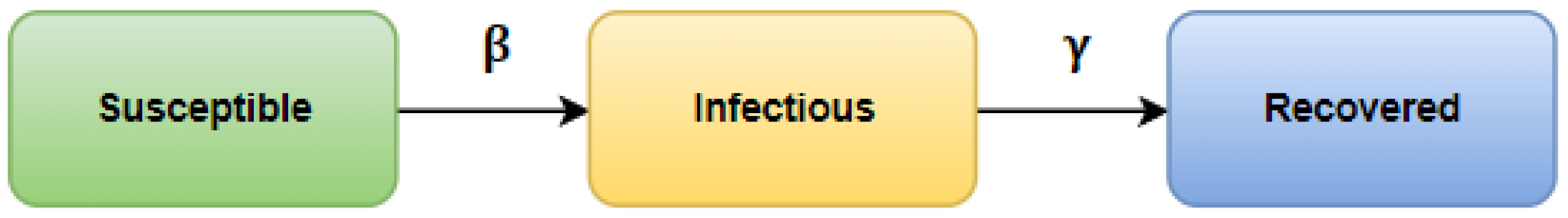
State changes. An actor in state S can change its state with probability to I if it has an infected neighbor. This model means that for each actor in the state I, all direct neighbors (all nodes connected by an edge to a given infected node) are searched; for each of them, a value between (0, 1) indicating the probability of infection is randomized that is compared with the value of the threshold . If the drawn value is less than the then this actor will change its state to I on the next epidemic day (iteration of the process). Otherwise, the state of the node will not change. A separate draw determines the change of state of an actor in the state I. When all neighbors of the infected individual are found, a probability value is generated from the interval (0, 1) for it and, similarly to the case described above, it is compared with . The change in state to R will occur only if the generated value is lower than the . If this does not happen, the actor remains in the state I and continues to infect.
It should be noted that a node that has changed its state to R cannot change it to I again. However, there are indeed reports of reinfection in the literature, but their percentage relative to all cases is so low that they are not included in this model.
Probabilities and . The coronavirus pandemic led to intensive work in the scientific community on modeling the epidemic. As a result, in the literature, one can find probability values for the model tailored to the modeling of the SARS-CoV-2 virus spreading. Most publications concern Asian countries, especially China, where the pandemic began, and European countries, where the epidemic further developed—causing paralysis of health services, resulting in serious illnesses or deaths of many people. These countries included Italy, Spain, France, and, to a lesser extent, Germany and Poland.
Based on the analysis of available works, as well as the available social networks and their density, it was decided to adopt four different probability values, the first three for Italy (
[
36],
[
37],
[
38]) and one for Poland (
[
36]).
2.3.2. Model
The spread of the virus is accompanied by the spread of awareness (information) of its existence. However, this is a process at least partly independent of the spread of the virus. For this reason, it is necessary to have two different models for both processes. For the spread of information about the virus, the -based model was adapted.
Previous research showed that despite the spreading of seasonal diseases such as cold or flu, the
model could be successfully adapted for the spread of different types of information, taking into account the process of forgetting [
13]. The states of the model can then be described as
U (unaware)—unaware of information (
S in
model) and
A (aware)—spreading information (
I in
model).
The change of states is determined by the probabilities and . To simplify the understanding of the interactions between the models, the probabilities will be denoted by symbols and , respectively.
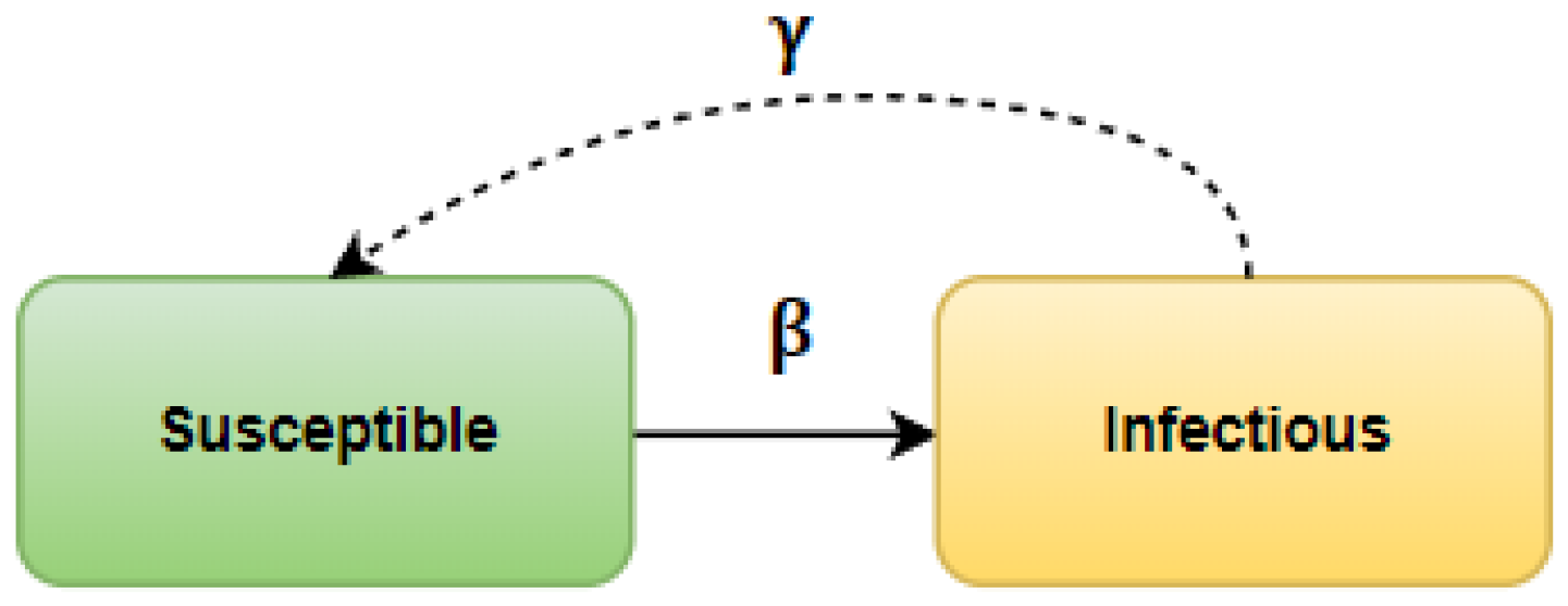
In the
model, an unaware actor in state
U may learn about the existence of the virus from a conscious member of the population
A. Over time, the aware person returns to state
U, which corresponds to the situation in which someone forgets about the existence of the virus or becomes used to it and awareness does not affect its behavior [
13]; for example, someone, despite knowing about the pandemic, stops wearing the mask. Similarly to the adaptation of the
model, for the
model, it was necessary to define the initial state and the assumptions.
Spreading structure. Simulating the spread of information requires defining the medium in which it will occur. Information and viruses in the real world coexist within the same population. Therefore, the network for the and models is common. However, the specifics of spreading differ. Unlike the virus, access to information is so widespread that receiving it does not require direct contact between two people. Information reaches the recipient through social networks, the Internet, newspapers, etc. However, this does not exclude acquiring information through real interpersonal contacts or traveling by shared means of transport. Furthermore, obtaining information from one source does not prevent encountering the same information again through another medium. Therefore, to simulate a real process, information may spread throughout the network at all layers. For simplicity, the type of interaction does not affect the entire process; regardless of the layer, the assumptions are the same.
Initial state. Similar to the infection process, information appears in a population through human action. To determine the initial state of the aware population, the same tactics were used as for the virus. Initially, one percent of all actors in the network are aware of the virus. The selection of informed actors results from random selection similar to the process.
State changes. An actor in state U can change its state to A with probability if it has an aware neighbor. What this model means is that for each actor in state U, all immediate neighbors (all nodes connected by an edge to a given aware vertex) are searched, and for each of them, a value is drawn from the interval (0, 1), denoting the probability of awareness. It is then compared with the value of the threshold . If the drawn value is less than the , the actor will change its state to A in the next iteration. Otherwise, the state of the individual will not change.
A separate drawing determines the change of state of an actor in state A. When all neighbors of the aware individual are found, then a probability value from the interval (0, 1) is drawn for it and, similar to the case described above, compared with the threshold, which is the probability . A return to state U will occur only if the drawn value is less than the . If this does not happen, the actor remains in state A and continues to spread information. A node that has changed its state to U may change it again to A. Although, over time, we forget a given piece of information or consciously downplay the presence of the virus, resulting in a return to state U, this does not preclude a renewed increase in interest or awareness.
Probabilities and
In previous research, we could not find information on how to determine the
and
for the
model during the spread of information about the SARS-CoV-2 virus. Therefore, it was assumed that the probabilities
and
would be equal to the probabilities of the
model to reflect the intensity of the spread of information and this issomehow related to the intensity of virus spread. Since in real life, the spread of information is much faster than the virus itself, it was decided to extend the set of probabilities by multiplying the initial probabilities according to the equations:
Thus, for each
and
combination, we have four combinations of
and
.
2.3.3. Interaction between Virus and Information Processes
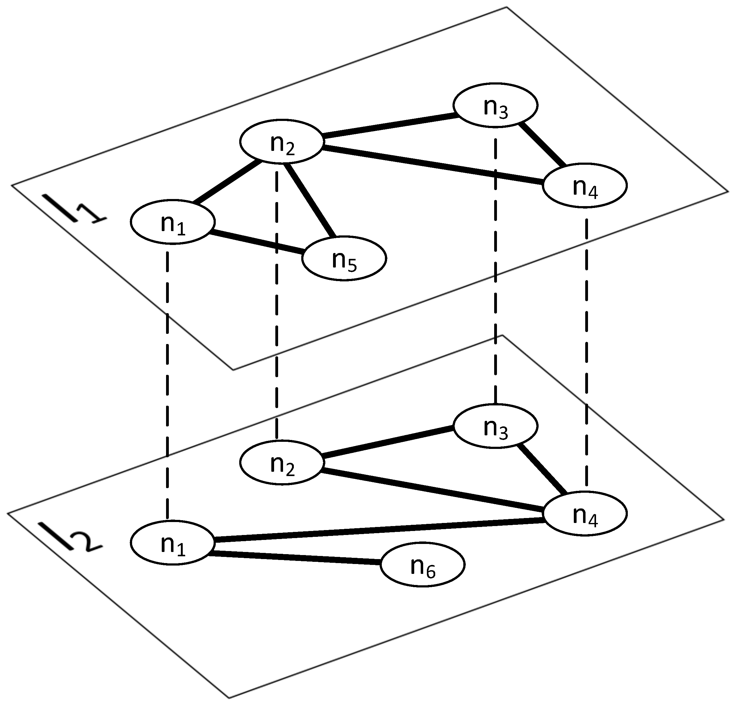
While analyzing the impact of the spread of information on the virus, it is necessary to locate both processes in a single medium. For this purpose, a multilayer network was chosen. The virus spread, simulated by the
model, will progress within a direct contact layer. In contrast, awareness will spread in all layers. Therefore, it is necessary to address the interaction between the models. In reality, awareness of the virus causes a range of behaviors designed to avoid infection (social distancing, masks, vaccination, etc.). A representation of this phenomenon will be a reduction in the infection probability,
, for actors aware of the virus. Choosing just one number for the reduction of
was difficult since different actions yield different results in infection risk reduction. For example, wearing a mask will result in 65% risk reduction (RR) [
39], and one meter of social distancing has a similar effect (RR of 65%) [
39,
40], with RR increasing with the distance [
39]. Other actions have lower (e.g., face shields) or higher RR (e.g., quarantine and self-isolation have RR of almost 100%). Additionally, one will increase RR with the combination of more than one action (e.g., face mask and social distancing). Since various countries decided on different actions and various actions have various effects we decided to assume RR of 90%. Thus, the primary probability will be reduced by a factor of ten, which the following equation can describe:
, where
is the probability of infection and
is the probability of infection of an aware node.
Similar to how awareness affects the probability of infection, the infection can alter the chance of becoming aware. This corresponds to the situation where a person with COVID-19 becomes aware of the SARS-CoV-2 virus by having specific disease symptoms or test results. However, not all cases of infection with the coronavirus are manifested by symptoms [
41,
42]. At the same time, symptoms can be similar to other upper respiratory diseases that are not difficult to confuse. To address the impact of this phenomenon on the
, the percentage of symptomatic patients was taken. In previous research on the SARS-CoV-2 virus, only a few addressed the issue of the number of asymptomatic patients. One of the most important is the proportion of patients with asymptomatic COVID-19 based on observations of passengers on the Diamond Princess, a quarantined ship off the coast of Wuhan. In this case, 17.9% of the ill passengers were asymptomatic [
41]. However, it should be noted that the ship’s crew, by sharing the quarantine, was an isolated community, so generalizing the results to the whole population might not be correct. Slightly more general results were obtained in a study of a group of Japanese people evacuated from Wuhan by a shared plane. Although the group examined was smaller than that of the ship’s passengers, a significant difference is the lack of shared isolation. Researchers, using a binomial distribution, estimated that among evacuees, the proportion of symptomless patients was 30.8% [
42]. The characteristics of the virus change over time due to mutations or certain individual attributes in different populations. However, since we are interested in the initial part of the pandemic, we can use published data from the initial period of the spread of the SARS-CoV-2 virus. Based on this, we assumed that the probability that the unaware node becomes aware if it is infected will correspond to the percentage of symptomatically ill people from [
42], i.e.,
. The described changes in probabilities are presented in
Table 2.
In summary, the interaction between information dissemination and virus spread can be classified as a mixed interaction. The virus spread supports information dissemination, and information dissemination can suppress virus spread. An example of support is increasing the chance of obtaining information about the virus for an infected node. This allows the information to spread faster.
Otherwise, knowledge of the existence of the virus reduces the chances of an actor being infected by blocking the development of an epidemic. This is an example of competition. It should be noted that competition is not limited to the layer where both processes occur because awareness of the virus gained in the layer of direct contacts affects the spread of information about the virus in all other layers.


