


Kernel-Based Independence Tests for Causal Structure Learning on Functional Data

 ,
,
Abstract
:1. Introduction
- In Section 4.1.2, we extend the historical functional linear model [20] to the multivariate case for regression-based causal structure learning, and we show how a joint independence test can be used to verify candidate directed acyclic graph (dags) ([21], § 5.2) that embed the causal structure of function-valued random variables. This model has been contributed to the Python package scikit-fda [22].
- On synthetic data, we show empirically that our bivariate, joint, and conditional independence tests achieve high test power, and that our causal structure learning algorithms outperform previously proposed methods.
- Using a real-world dataset (World Governance Indicators), we demonstrate how our method can yield insights into cause–effect relationships amongst socioeconomic variables measured in countries worldwide.
- Implementations of our algorithms are made available at https://github.com/felix-laumann/causal-fda/ (accessed on 10 October 2023) in an easily usable format that builds on top of scikit-fda and causaldag [23].
2. Background and Related Work
2.1. Functional Data Analysis
2.2. Kernel Independence Tests
2.3. Causal Structure Learning
- Score-based approaches assign a score, such as a penalised likelihood, to each candidate graph and then pick the highest scoring graph(s). A common drawback of score-based approaches is the need for a combinatorial enumeration of all dags in the optimisation, although greedy approaches have been proposed to alleviate such issues [41].
- Constraint-based methods start by characterising the set of conditional independences in the observed data [14]. They then determine the graph(s) consistent with the detected conditional independences by using a graphical criterion called d-separation, as well as the causal Markov and faithfulness assumptions, which establish a one-to-one connection between d-separation and conditional independence (see Appendix B for definitions). When only observational i.i.d. data are available, this yields a so-called Markov equivalence class, possibly containing multiple candidate graphs. For example, the graphs , , and are Markov equivalent, as they all imply and no other conditional independence relations.
- Regression-based approaches directly fit the structural equations of an underlying scm for each , where denote the parents of in the causal dag and are jointly independent exogenous noise variables. Provided that the function class of the is sufficiently restricted, e.g., by considering only linear relationships [42] or additive noise models [43], the true causal graph is identified as the unique choice of parents for each i such that the resulting residuals are jointly independent.
3. Methods
3.1. Conditional Independence Test on Functional Data
 can be rejected. Given that both the evaluation test statistic and the evaluation null statistics are computed on conditionally independent samples, we repeat this procedure for times to estimate an evaluation rejection rate for each value of . Having completed this procedure over all values , we select the that produces an evaluation rejection rate closest to as the optimised regularisation strength, . Finally, we apply a cpt-based conditional independence test using the optimised to test the null hypothesis
  . This entire procedure is summarised in Algorithm 1.
| Algorithm 1 Search for with subsequent conditional independence test | |
| Require: Samples (), Range , Significance level , Permutation iterations P, Rejection iterations B | |
| Initalise: | |
| 1: | for do ▹Start: Search for |
| 2: | for do |
| 3: | Permute by cpt, call them |
| 4: | |
| 5: | for do |
| 6: | Permute by cpt, call them |
| 7: | |
| 8: | |
| 9: | |
| 10: | if then |
| 11: | Fail to reject |
| 12: | rejects |
| 13: | else |
| 14: | Reject  |
| 15: | |
| 16: | |
| 17: | if then |
| 18: | |
| 19: | return ▹End: Search for |
| 20: | ▹Start: Conditional independence test |
| 21: | for do |
| 22: | Permute by cpt, call them |
| 23: | |
| 24: | |
| 25: | if then |
| 26: | Fail to reject |
| 27: | else |
| 28: | Reject  |
| ▹End: Conditional independence test | |
3.2. Causal Structure Learning on Functional Data
3.2.1. Constraint-Based Causal Structure Learning
 , we can orient the edges and to form colliders (or v-structures), .
3.2.2. Regression-Based Causal Structure Learning
4. Experiments
4.1. Evaluation of Independence Tests for Functional Data
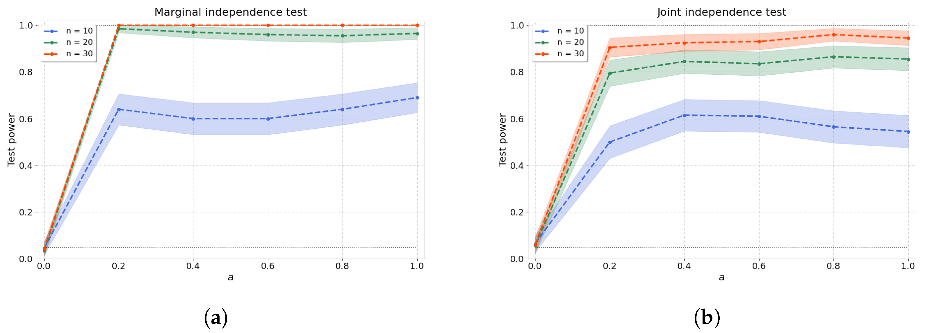
4.1.1. Bivariate Independence Test
4.1.2. Joint Independence Test
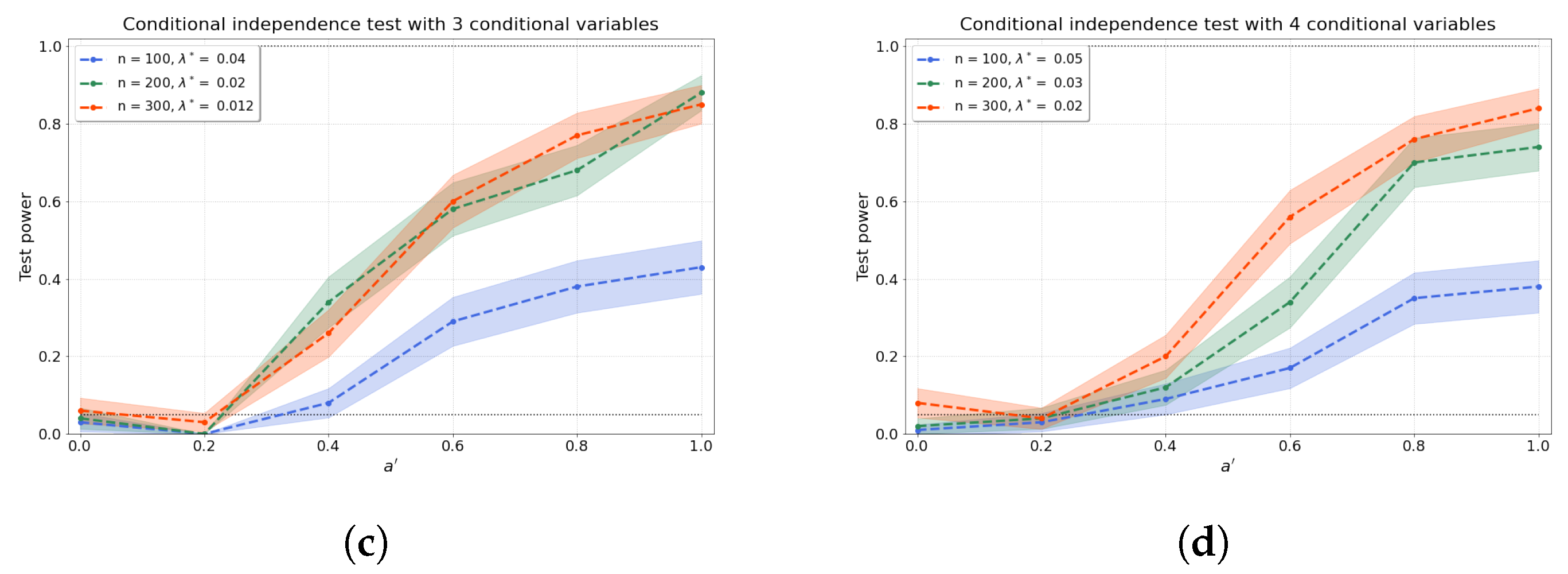
4.1.3. Conditional Independence Test
4.2. Causal Structure Learning
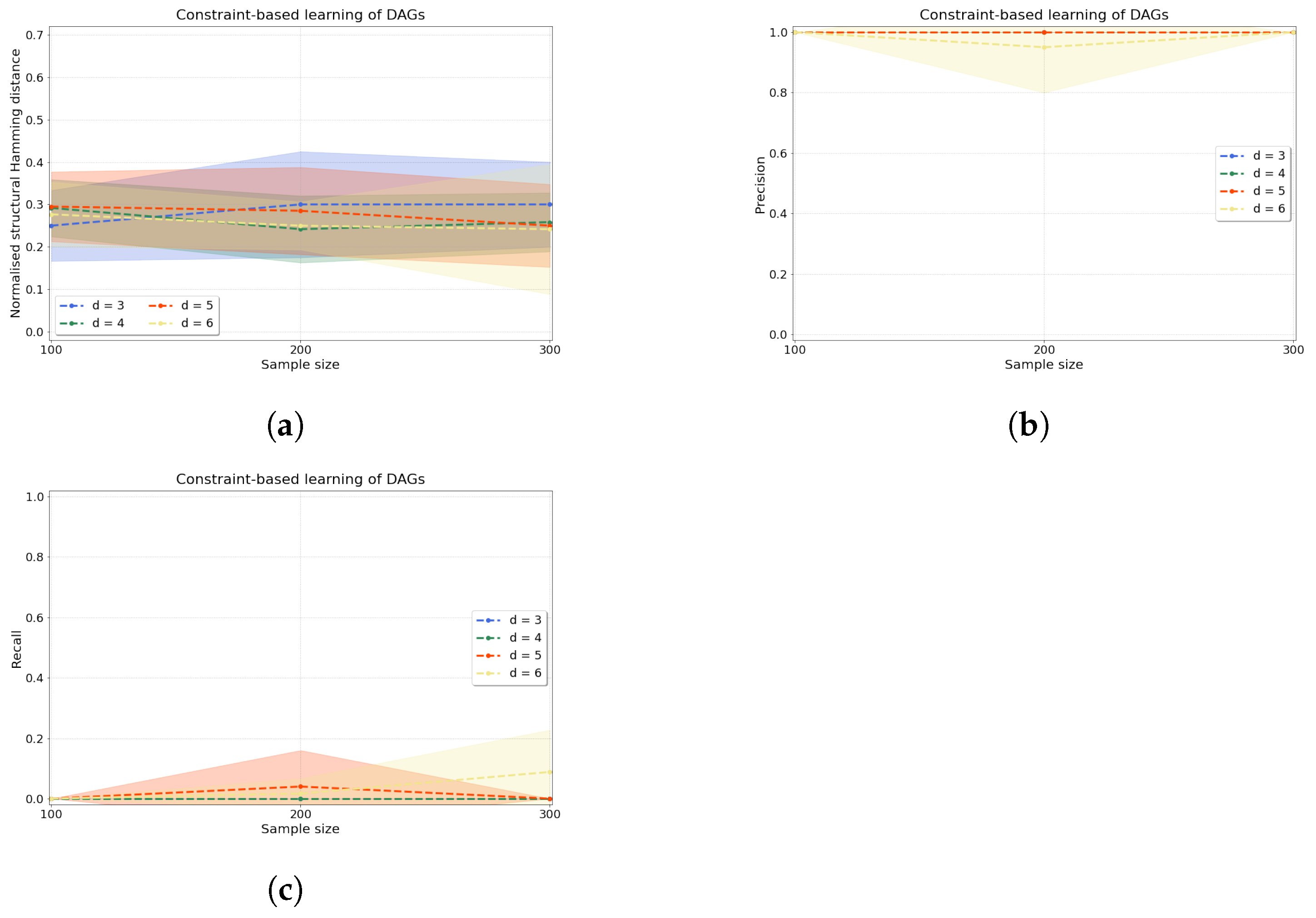
4.2.1. Synthetic Data
4.2.2. Real-World Data
5. Discussion and Conclusions
Author Contributions
Funding
Data Availability Statement
Conflicts of Interest
Appendix A. Proof of Theorem 1
Appendix B. Additional Definitions for Causal Learning
Appendix B.1. d-Separation
Appendix B.2. Faithfulness Assumption
Appendix B.3. Causal Markov Assumption
Appendix C. Meek’s Orientation Rules, the SGS and the PC Algorithms
- Form the complete undirected graph G from the set of vertices (or nodes) .
- For each pair of vertices X and Y, if there exists a subset S of such that X and Y are d-separated, i.e., conditionally independent (causal Markov condition), given Z, remove the edge between X and Y from G.
- Let K be the undirected graph resulting from the previous step 2. For each triple of vertices X, Y, and Z such that the pair X and Y and the pair Y and Z are each adjacent in K (written as ) but the pair X and Z are not adjacent in K, orient as if—and only if—there is no subset S of Y that d-separates X and Z.
- Repeat the following steps until no more edges can be oriented:
- (a)
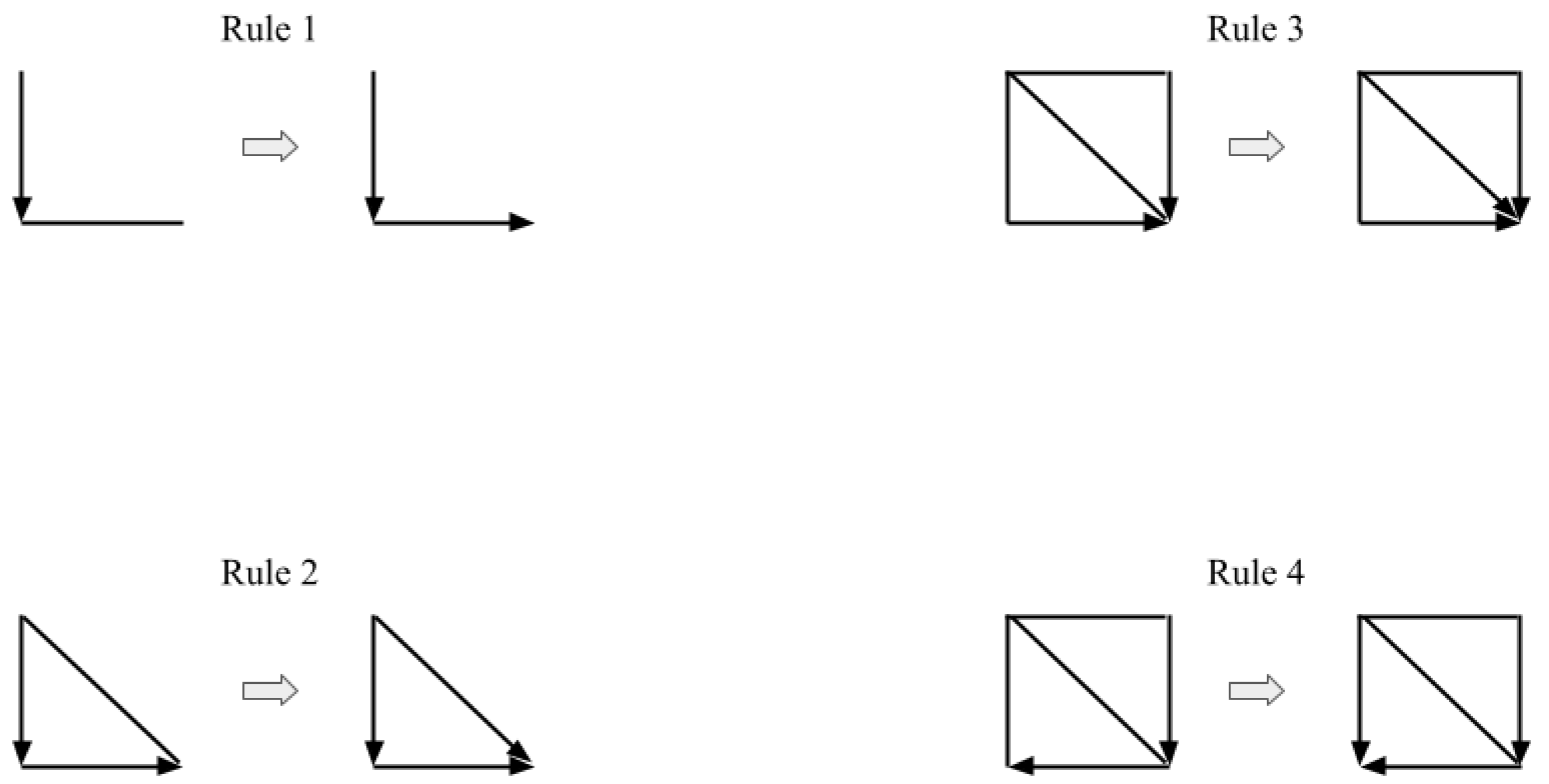
- If , Y and Z are adjacent, X and Z are not adjacent, and there is no arrowhead of other vertices at Y, then orient as (Rule 1 of Meek’s orientation rules).
- (b)
- If there is a directed path over some other vertices from X to Y, and an edge between X and Y, then orient as (Rule 2 of Meek’s orientation rules).

Appendix D. Definitions of Performance Metrics
Appendix D.1. shd
Appendix D.2. Normalised shd
Appendix D.3. Precision
Appendix D.4. Recall
Appendix E. Other Causal Methods Used for Comparison
Appendix E.1. Granger causality
Appendix E.2. ccm
Appendix E.3. pcmci
Appendix F. Computational Complexity of Our Proposed Methods
Appendix F.1. Regression-Based Causal Discovery
Appendix F.2. Constraint-Based Approach
Appendix G. Comparison of Running Times of Our Proposed Method and the Other Causal Methods

| d | Regression-Based | Constraint-Based | Combined | Granger Causality | CCM | PCMCI |
|---|---|---|---|---|---|---|
| 2 | 1 min 57 s | – | – | 998 ms | 1.57 s | – |
| 3 | 30 min 35 s | 1 min 10 s | 3 min 13 s | 43 s | – | 45.5 s |
| 4 | – | 8 min 10 s | 8 min 1 s | 1 min 23 s | – | 1 min 29 s |
| 5 | – | 34 min 33 s | 39 min 8 s | 2 min 44 s | – | 2 min 50 s |
| 6 | – | 1 h 31 min 36 s | 1 h 43 min 54 s | 3 min 20 s | – | 3 min 27 s |
Appendix H. Influence of Nonlinearity and Nonstationarity on Granger Causality and ccm
Appendix H.1. Nonlinearity and Granger Causality:

Appendix H.2. Nonstationarity and ccm:

Appendix I. World Governance Indicators
| Abbreviation | Official Name | Description |
|---|---|---|
| VA | Voice and Accountability | Voice and accountability captures perceptions of the extent to which a country’s citizens are able to participate in selecting their government, as well as freedom of expression, freedom of association, and a free media. |
| PS | Political Stability and No Violence | Political Stability and Absence of Violence/Terrorism measures perceptions of the likelihood of political instability and/or politically-motivated violence, including terrorism. |
| GE | Government Effectiveness | Government effectiveness captures perceptions of the quality of public services, the quality of the civil service and the degree of its independence from political pressures, the quality of policy formulation and implementation, and the credibility of the government’s commitment to such policies. |
| RQ | Regulatory Quality | Regulatory quality captures perceptions of the ability of the government to formulate and implement sound policies and regulations that permit and promote private sector development. |
| RL | Rule of Law | Rule of law captures perceptions of the extent to which agents have confidence in and abide by the rules of society, and in particular the quality of contract enforcement, property rights, the police, and the courts, as well as the likelihood of crime and violence. |
| CC | Control of Corruption | Control of corruption captures perceptions of the extent to which public power is exercised for private gain, including both petty and grand forms of corruption, as well as “capture” of the state by elites and private interests. |
References
- Runge, J.; Bathiany, S.; Bollt, E.; Camps-Valls, G.; Coumou, D.; Deyle, E.; Glymour, C.; Kretschmer, M.; Mahecha, M.D.; Muñoz-Marí, J.; et al. Inferring causation from time series in Earth system sciences. Nat. Commun. 2019, 10, 2553. [Google Scholar] [CrossRef] [PubMed]
- Sulemana, I.; Kpienbaareh, D. An empirical examination of the relationship between income inequality and corruption in Africa. Econ. Anal. Policy 2018, 60, 27–42. [Google Scholar] [CrossRef]
- Finkle, J.D.; Wu, J.J.; Bagheri, N. Windowed granger causal inference strategy improves discovery of gene regulatory networks. Proc. Natl. Acad. Sci. USA 2018, 115, 2252–2257. [Google Scholar] [CrossRef]
- Glymour, C.; Zhang, K.; Spirtes, P. Review of causal discovery methods based on graphical models. Front. Genet. 2019, 10, 524. [Google Scholar] [CrossRef]
- Ramsay, J.O. Functional Data Analysis, 2nd ed.; Springer series in statistics; Springer: New York, NY, USA, 2005. [Google Scholar]
- Granger, C.W. Investigating causal relations by econometric models and cross-spectral methods. Econom. J. Econom. Soc. 1969, 37, 424–438. [Google Scholar] [CrossRef]
- Geweke, J. Measurement of linear dependence and feedback between multiple time series. J. Am. Stat. Assoc. 1982, 77, 304–313. [Google Scholar] [CrossRef]
- Sugihara, G.; May, R.; Ye, H.; Hsieh, C.h.; Deyle, E.; Fogarty, M.; Munch, S. Detecting causality in complex ecosystems. Science 2012, 338, 496–500. [Google Scholar] [CrossRef]
- Kaufmann, D.; Kraay, A.; Mastruzzi, M. The worldwide governance indicators: Methodology and analytical issues. Hague J. Rule Law 2011, 3, 220–246. [Google Scholar] [CrossRef]
- World Bank. Gini Index. 2022. Available online: https://data.worldbank.org/indicator/SI.POV.GINI (accessed on 7 June 2023).
- Jong-Sung, Y.; Khagram, S. A comparative study of inequality and corruption. Am. Sociol. Rev. 2005, 70, 136–157. [Google Scholar] [CrossRef]
- Alesina, A.; Angeletos, G.M. Corruption, inequality, and fairness. J. Monet. Econ. 2005, 52, 1227–1244. [Google Scholar] [CrossRef]
- Dobson, S.; Ramlogan-Dobson, C. Is there a trade-off between income inequality and corruption? Evidence from Latin America. Econ. Lett. 2010, 107, 102–104. [Google Scholar] [CrossRef]
- Spirtes, P.; Glymour, C.N.; Scheines, R.; Heckerman, D. Causation, Prediction, and Search; MIT Press: Cambridge, MA, USA, 2000. [Google Scholar]
- Peters, J.; Mooij, J.M.; Janzing, D.; Schölkopf, B. Causal discovery with continuous additive noise models. J. Mach. Learn. Res. 2014, 15, 2009–2053. [Google Scholar]
- Muandet, K.; Fukumizu, K.; Sriperumbudur, B.; Schölkopf, B. Kernel mean embedding of distributions: A review and beyond. Found. Trends Mach. Learn. 2017, 10, 1–141. [Google Scholar] [CrossRef]
- Wynne, G.; Duncan, A.B. A kernel two-sample test for functional data. J. Mach. Learn. Res. 2022, 23, 1–51. [Google Scholar]
- Park, J.; Muandet, K. A measure-theoretic approach to kernel conditional mean embeddings. Adv. Neural Inf. Process. Syst. 2020, 33, 21247–21259. [Google Scholar]
- Berrett, T.B.; Wang, Y.; Barber, R.F.; Samworth, R.J. The conditional permutation test for independence while controlling for confounders. J. R. Stat. Soc. Ser. B Stat. Methodol. 2020, 82, 175–197. [Google Scholar] [CrossRef]
- Malfait, N.; Ramsay, J.O. The historical functional linear model. Can. J. Stat. 2003, 31, 115–128. [Google Scholar] [CrossRef]
- Pfister, N.; Bühlmann, P.; Schölkopf, B.; Peters, J. Kernel-based tests for joint independence. J. R. Stat. Soc. Ser. B Stat. Methodol. 2018, 80, 5–31. [Google Scholar] [CrossRef]
- Ramos-Carreño, C.; Suárez, A.; Torrecilla, J.L.; Carbajo Berrocal, M.; Marcos Manchón, P.; Pérez Manso, P.; Hernando Bernabé, A.; García Fernández, D.; Hong, Y.; Rodríguez-Ponga Eyriès, P.M.; et al. GAA-UAM/scikit-fda: Version 0.7.1. 2022. Available online: https://zenodo.org/records/5903557(accessed on 7 June 2023).
- Squires, C. Causaldag: Creation, Manipulation, and Learning of Causal Models. 2018. Available online: https://github.com/uhlerlab/causaldag (accessed on 7 June 2023).
- Girard, O.; Lattier, G.; Micallef, J.P.; Millet, G.P. Changes in exercise characteristics, maximal voluntary contraction, and explosive strength during prolonged tennis playing. Br. J. Sport. Med. 2006, 40, 521–526. [Google Scholar] [CrossRef]
- Zhu, Y.; Kuhn, T.; Mayo, P.; Hinds, W.C. Comparison of daytime and nighttime concentration profiles and size distributions of ultrafine particles near a major highway. Environ. Sci. Technol. 2006, 40, 2531–2536. [Google Scholar] [CrossRef]
- Ramsay, J.; Hooker, G. Dynamic Data Analysis; Springer: Berlin/Heidelberg, Germany, 2017. [Google Scholar]
- Fukumizu, K.; Gretton, A.; Sun, X.; Schölkopf, B. Kernel measures of conditional dependence. In Proceedings of the 20th International Conference on Neural Information Processing Systems, Vancouver, BC, Canada, 3–6 December 2007. [Google Scholar]
- Gretton, A.; Fukumizu, K.; Teo, C.H.; Song, L.; Schölkopf, B.; Smola, A.J. A kernel statistical test of independence. In Proceedings of the 20th International Conference on Neural Information Processing Systems, Vancouver, BC, Canada, 3–6 December 2007; pp. 585–592. [Google Scholar]
- Zhang, K.; Peters, J.; Janzing, D.; Schölkopf, B. Kernel-based conditional independence test and application in causal discovery. arXiv 2012, arXiv:1202.3775. [Google Scholar]
- Lai, T.; Zhang, Z.; Wang, Y.; Kong, L. Testing independence of functional variables by angle covariance. J. Multivar. Anal. 2021, 182, 104711. [Google Scholar] [CrossRef]
- Górecki, T.; Krzyśko, M.; Wołyński, W. Independence test and canonical correlation analysis based on the alignment between kernel matrices for multivariate functional data. Artif. Intell. Rev. 2020, 53, 475–499. [Google Scholar] [CrossRef]
- Doran, G.; Muandet, K.; Zhang, K.; Schölkopf, B. A Permutation-Based Kernel Conditional Independence Test. In Proceedings of the Thirtieth Conference on Uncertainty in Artificial Intelligence, Quebec City, QC, Canada, 23–27 July 2014; pp. 132–141. [Google Scholar]
- Gretton, A.; Borgwardt, K.M.; Rasch, M.J.; Schölkopf, B.; Smola, A. A kernel two-sample test. J. Mach. Learn. Res. 2012, 13, 723–773. [Google Scholar]
- Lee, S.; Honavar, V.G. Self-discrepancy conditional independence test. In Proceedings of the 33rd Conference on Uncertainty in Artificial Intelligence, UAI 2017, Sydney, Australia, 11–15 August 2017; Volume 33. [Google Scholar]
- Pearl, J. Causality; Cambridge University Press: Cambridge, UK, 2009. [Google Scholar]
- Mooij, J.M.; Peters, J.; Janzing, D.; Zscheischler, J.; Schölkopf, B. Distinguishing cause from effect using observational data: Methods and benchmarks. J. Mach. Learn. Res. 2016, 17, 1103–1204. [Google Scholar]
- Peters, J.; Janzing, D.; Schölkopf, B. Elements of Causal Inference; The MIT Press: Cambridge, MA, USA, 2017. [Google Scholar]
- Schölkopf, B.; von Kügelgen, J. From statistical to causal learning. arXiv 2022, arXiv:2204.00607. [Google Scholar]
- Squires, C.; Uhler, C. Causal structure learning: A combinatorial perspective. Found. Comput. Math. 2023, 23, 1781–1815. [Google Scholar] [CrossRef]
- Vowels, M.J.; Camgoz, N.C.; Bowden, R. D’ya like dags? A survey on structure learning and causal discovery. ACM Comput. Surv. 2022, 55, 1–36. [Google Scholar] [CrossRef]
- Chickering, D.M. Optimal structure identification with greedy search. J. Mach. Learn. Res. 2002, 3, 507–554. [Google Scholar]
- Shimizu, S.; Hoyer, P.O.; Hyvärinen, A.; Kerminen, A.; Jordan, M. A linear non-Gaussian acyclic model for causal discovery. J. Mach. Learn. Res. 2006, 7, 2003–2030. [Google Scholar]
- Hoyer, P.; Janzing, D.; Mooij, J.M.; Peters, J.; Schölkopf, B. Nonlinear causal discovery with additive noise models. In Proceedings of the 21st International Conference on Neural Information Processing Systems, Vancouver, BC, Canada, 8–10 December 2008. [Google Scholar]
- Szabó, Z.; Sriperumbudur, B.K. Characteristic and Universal Tensor Product Kernels. J. Mach. Learn. Res. 2017, 18, 1–29. [Google Scholar]
- Meek, C. Complete Orientation Rules for Patterns; Carnegie Mellon, Department of Philosophy: Pittsburgh, PA, USA, 1995. [Google Scholar]
- Peters, J.; Mooij, J.; Janzing, D.; Schölkopf, B. Identifiability of causal graphs using functional models. arXiv 2012, arXiv:1202.3757. [Google Scholar]
- Bühlmann, P.; Peters, J.; Ernest, J. CAM: Causal additive models, high-dimensional order search and penalized regression. Ann. Statist. 2014, 42, 2526–2556. [Google Scholar] [CrossRef]
- Shah, R.D.; Peters, J. The hardness of conditional independence testing and the generalised covariance measure. Ann. Stat. 2020, 48, 1514–1538. [Google Scholar] [CrossRef]
- Runge, J.; Nowack, P.; Kretschmer, M.; Flaxman, S.; Sejdinovic, D. Detecting and quantifying causal associations in large nonlinear time series datasets. Sci. Adv. 2019, 5, eaau4996. [Google Scholar] [CrossRef] [PubMed]
- Gini, C. On the measure of concentration with special reference to income and statistics. Colo. Coll. Publ. Gen. Ser. 1936, 208, 73–79. [Google Scholar]
- Ye, H.; Deyle, E.R.; Gilarranz, L.J.; Sugihara, G. Distinguishing time-delayed causal interactions using convergent cross mapping. Sci. Rep. 2015, 5, 14750. [Google Scholar] [CrossRef] [PubMed]
- Rulkov, N.F.; Sushchik, M.M.; Tsimring, L.S.; Abarbanel, H.D. Generalized synchronization of chaos in directionally coupled chaotic systems. Phys. Rev. E 1995, 51, 980. [Google Scholar] [CrossRef]
- Barnett, L.; Barrett, A.B.; Seth, A.K. Granger causality and transfer entropy are equivalent for Gaussian variables. Phys. Rev. Lett. 2009, 103, 238701. [Google Scholar] [CrossRef]
- Porta, A.; Faes, L.; Nollo, G.; Bari, V.; Marchi, A.; De Maria, B.; Takahashi, A.C.; Catai, A.M. Conditional self-entropy and conditional joint transfer entropy in heart period variability during graded postural challenge. PLoS ONE 2015, 10, e0132851. [Google Scholar]
- Van der Vaart, A.W. Asymptotic Statistics; Cambridge University Press: Cambridge, UK, 2000; Volume 3. [Google Scholar]
- Peters, J.; Bühlmann, P. Structural intervention distance for evaluating causal graphs. Neural Comput. 2015, 27, 771–799. [Google Scholar] [CrossRef] [PubMed]
- Seabold, S.; Perktold, J. Statsmodels: Econometric and statistical modeling with Python. In Proceedings of the 9th Python in Science Conference (SCIPY 2010), Austin, TX, USA, 28–30 June 2010. [Google Scholar]
- Javier, P.J.E. Causal-ccm: A Python Implementation of Convergent Cross Mapping. 2021. Available online: https://github.com/PrinceJavier/causal_ccm (accessed on 12 July 2021).
- Munch, E.; Khasawneh, F.; Myers, A.; Yesilli, M.; Tymochko, S.; Barnes, D.; Guzel, I.; Chumley, M. Teaspoon: Topological Signal Processing in Python. 2022. Available online: https://teaspoontda.github.io/teaspoon/ (accessed on 12 July 2022).
- Székely, G.J.; Rizzo, M.L.; Bakirov, N.K. Measuring and testing dependence by correlation of distances. Ann. Statist. 2007, 35, 2769–2794. [Google Scholar] [CrossRef]


Disclaimer/Publisher’s Note: The statements, opinions and data contained in all publications are solely those of the individual author(s) and contributor(s) and not of MDPI and/or the editor(s). MDPI and/or the editor(s) disclaim responsibility for any injury to people or property resulting from any ideas, methods, instructions or products referred to in the content. |
© 2023 by the authors. Licensee MDPI, Basel, Switzerland. This article is an open access article distributed under the terms and conditions of the Creative Commons Attribution (CC BY) license (https://creativecommons.org/licenses/by/4.0/).
Share and Cite
Laumann, F.; von Kügelgen, J.; Park, J.; Schölkopf, B.; Barahona, M. Kernel-Based Independence Tests for Causal Structure Learning on Functional Data. Entropy 2023, 25, 1597. https://doi.org/10.3390/e25121597
Laumann F, von Kügelgen J, Park J, Schölkopf B, Barahona M. Kernel-Based Independence Tests for Causal Structure Learning on Functional Data. Entropy. 2023; 25(12):1597. https://doi.org/10.3390/e25121597
Chicago/Turabian StyleLaumann, Felix, Julius von Kügelgen, Junhyung Park, Bernhard Schölkopf, and Mauricio Barahona. 2023. "Kernel-Based Independence Tests for Causal Structure Learning on Functional Data" Entropy 25, no. 12: 1597. https://doi.org/10.3390/e25121597
APA StyleLaumann, F., von Kügelgen, J., Park, J., Schölkopf, B., & Barahona, M. (2023). Kernel-Based Independence Tests for Causal Structure Learning on Functional Data. Entropy, 25(12), 1597. https://doi.org/10.3390/e25121597