

Refined Composite Multiscale Fuzzy Dispersion Entropy and Its Applications to Bearing Fault Diagnosis


Abstract
:1. Introduction
2. Methods
2.1. Multiscale Fuzzy Dispersion Entropy
2.1.1. Coarse-Graining
2.1.2. Multiscale Fuzzy Dispersion Entropy Calculation
2.1.3. Fuzzy Dispersion Entropy
- There is no boundary at the starting points of class 1 and end points of class c with other classes. Therefore, if is lower than 1 and higher than c, its degree of membership to classes 1 and c is equal to 1.
- The sum of the membership values of in different classes must be equal to 1.
- For a series of random numbers, the fuzzy membership functions possess equal relative cardinality.
- The overlap of the fuzzy membership function of each class with that of the adjoining classes can be 1 at most.
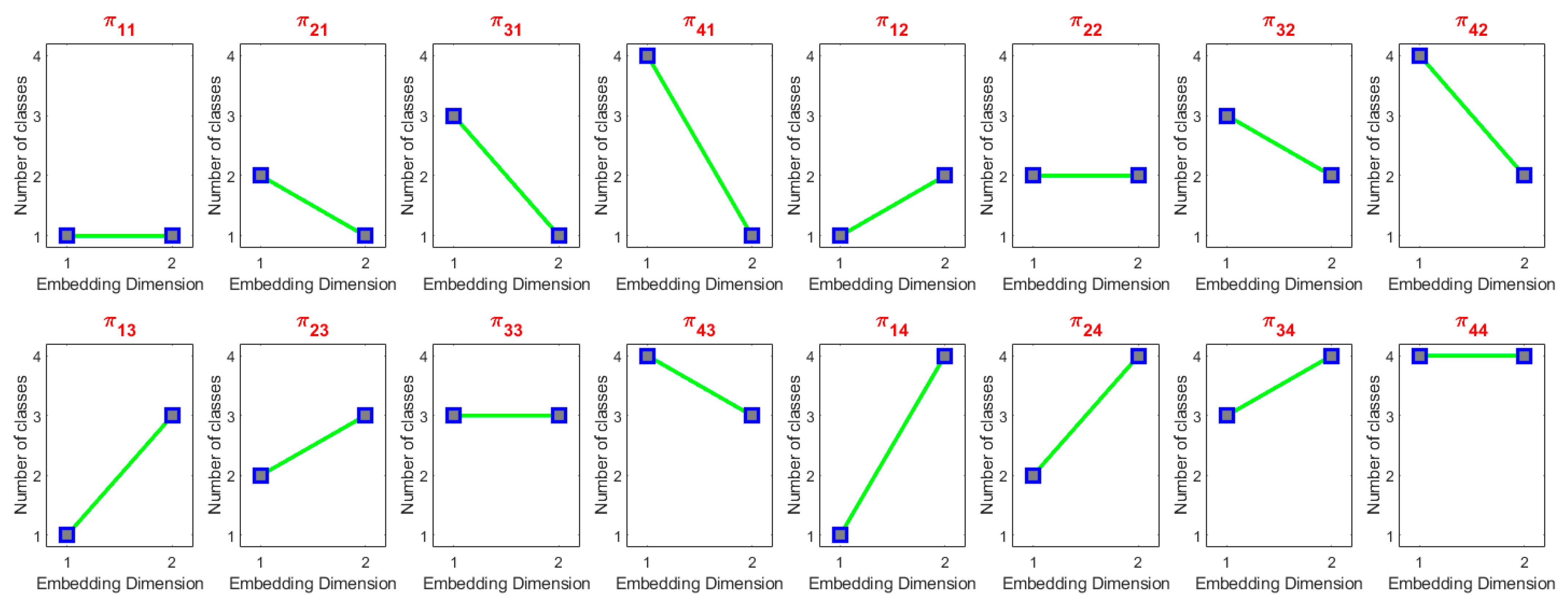
2.2. Refined Composite Multiscale Fuzzy Dispersion Entropy
3. Evaluation Signals
3.1. Synthetic Signals
3.1.1. White Gaussian Noise and Noise
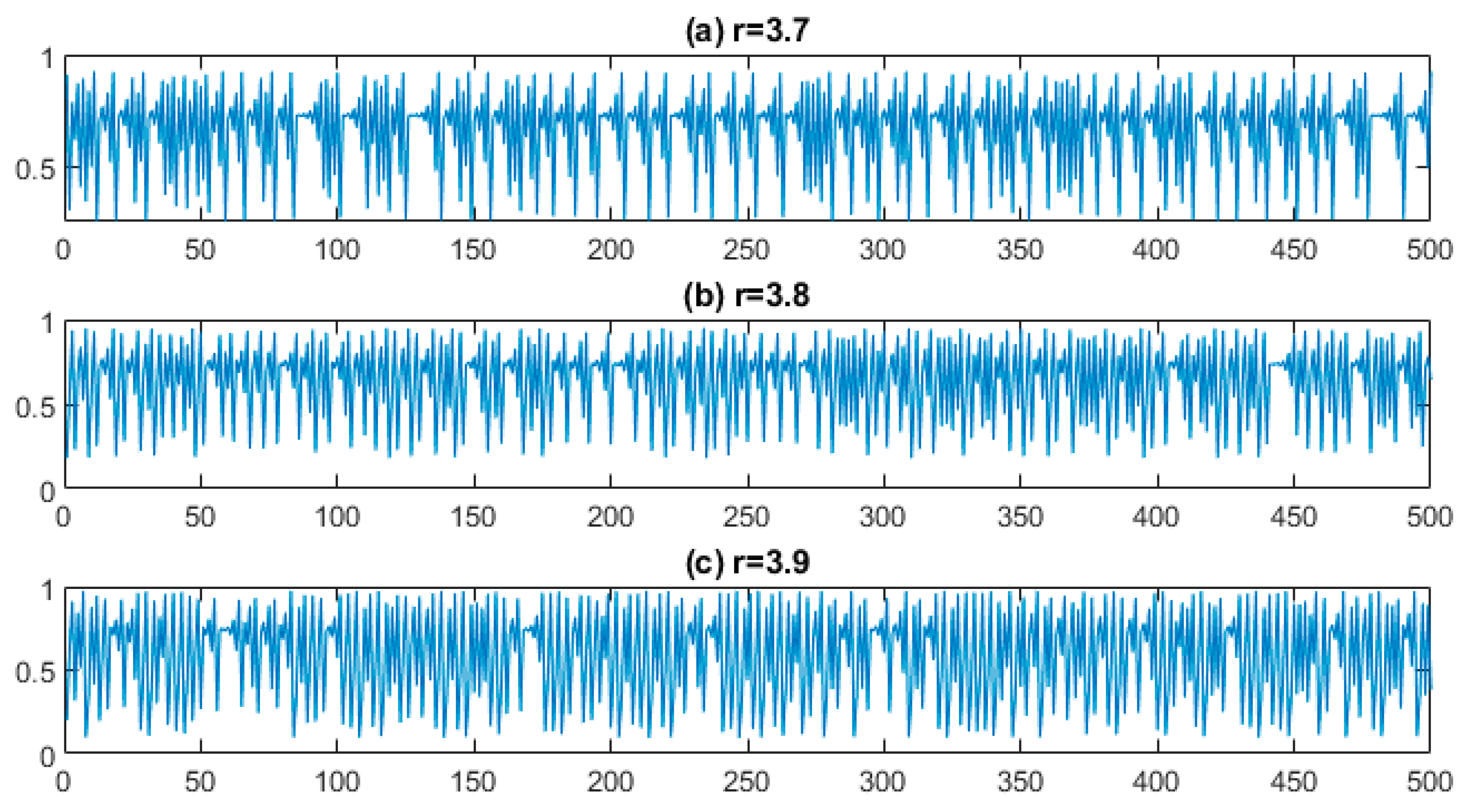
3.1.2. Logistic Map
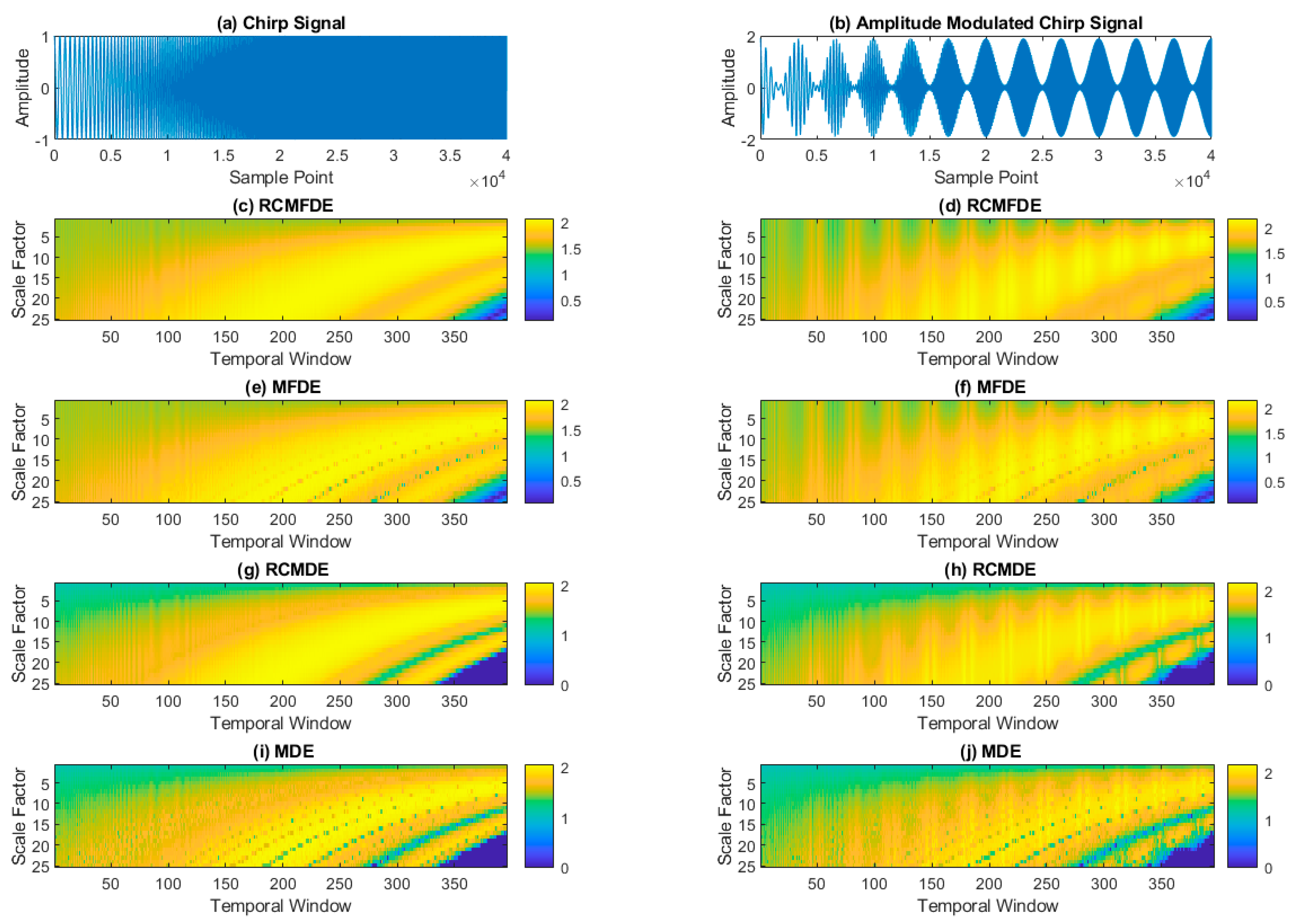
3.1.3. Chirp Signal and Amplitude-Modulated Chirp Signal
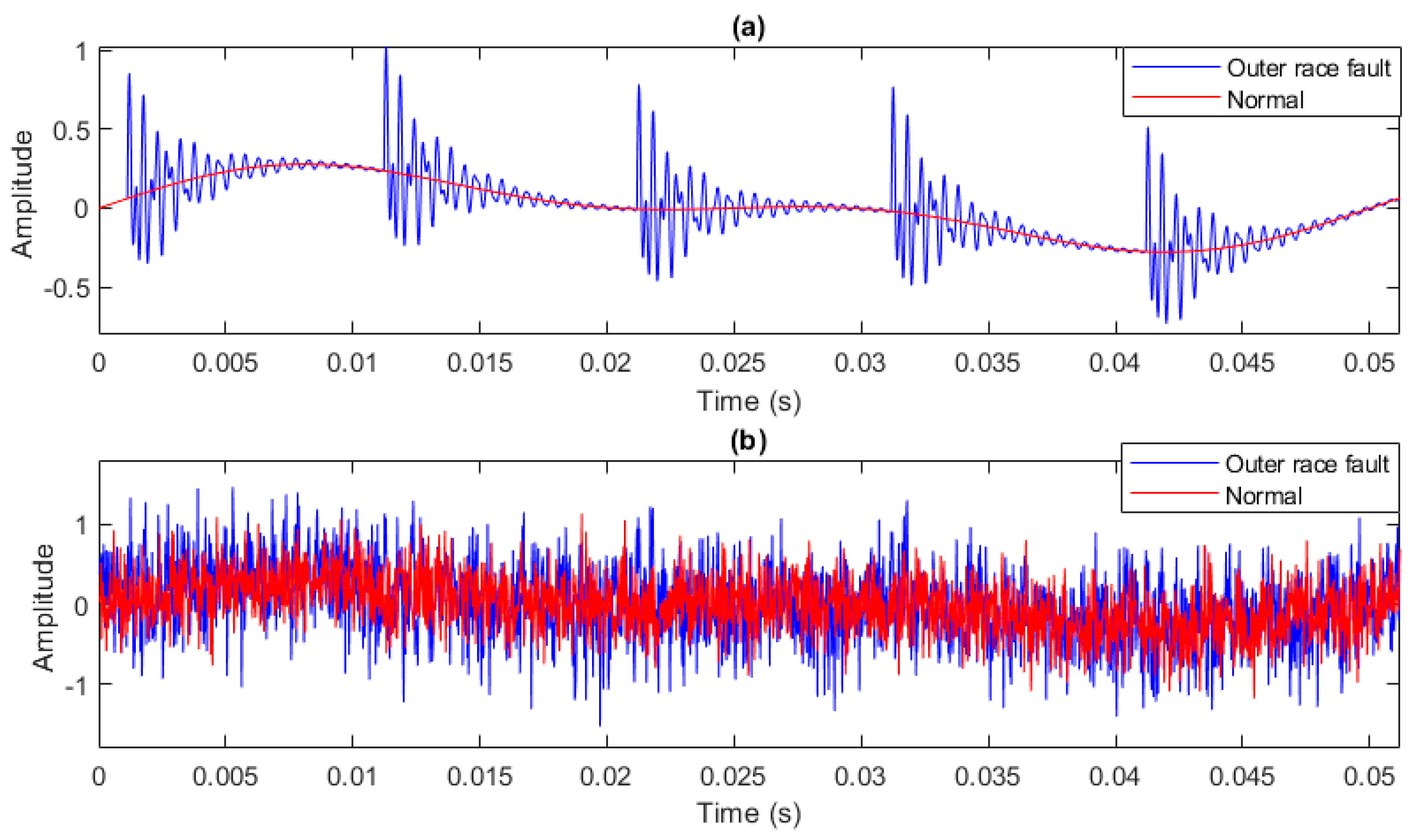
3.1.4. Faulty Bearing Simulation
3.2. Bearing Datasets
3.2.1. Paderborn University Dataset
3.2.2. PHMAP 2021 Data Challenge Dataset
3.2.3. Case Western Reserve University Dataset
4. Results and Discussion
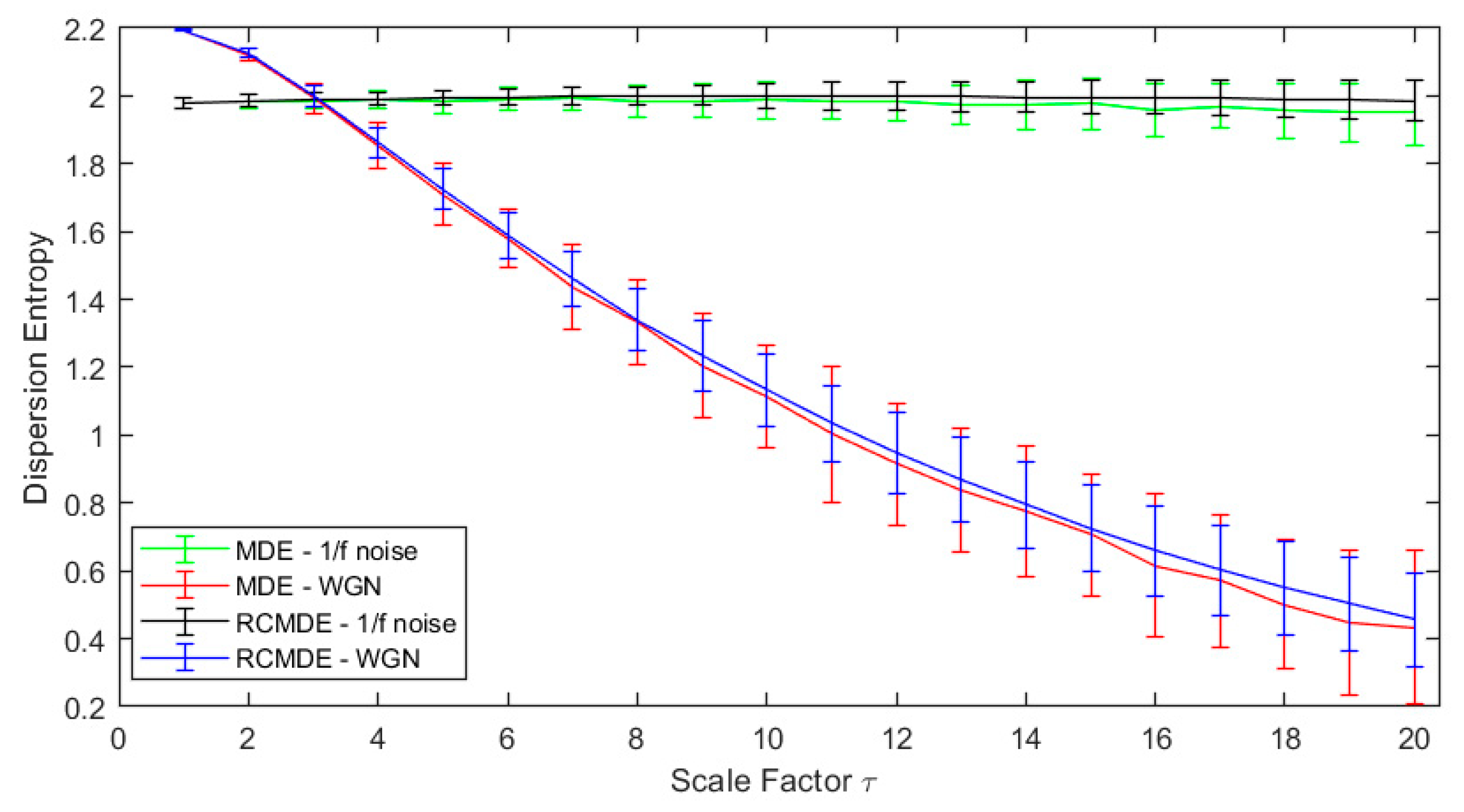
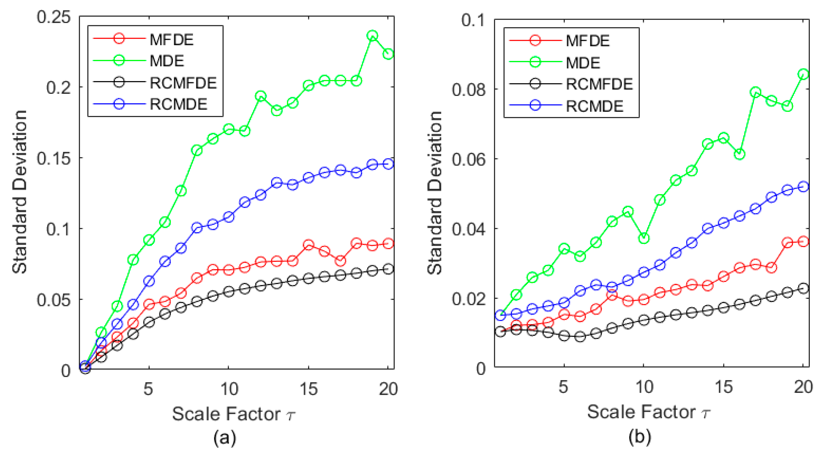
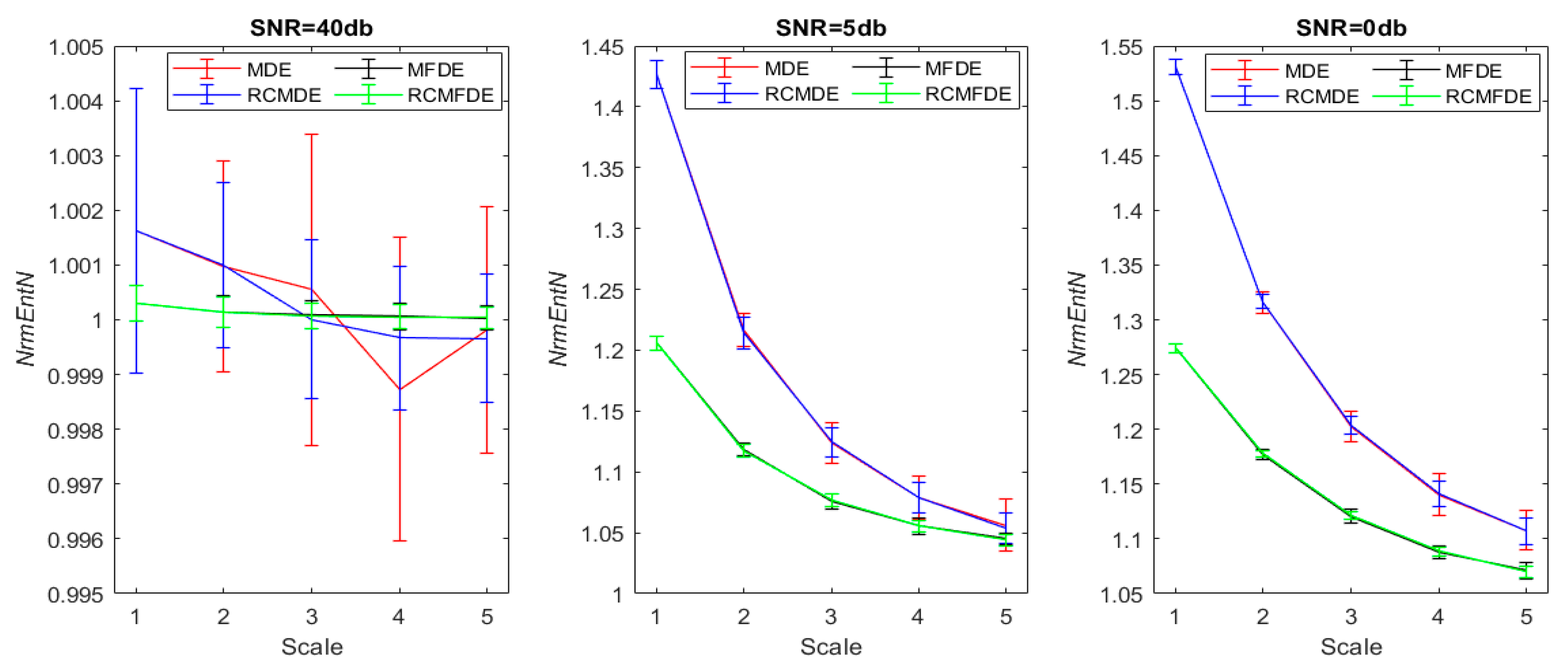
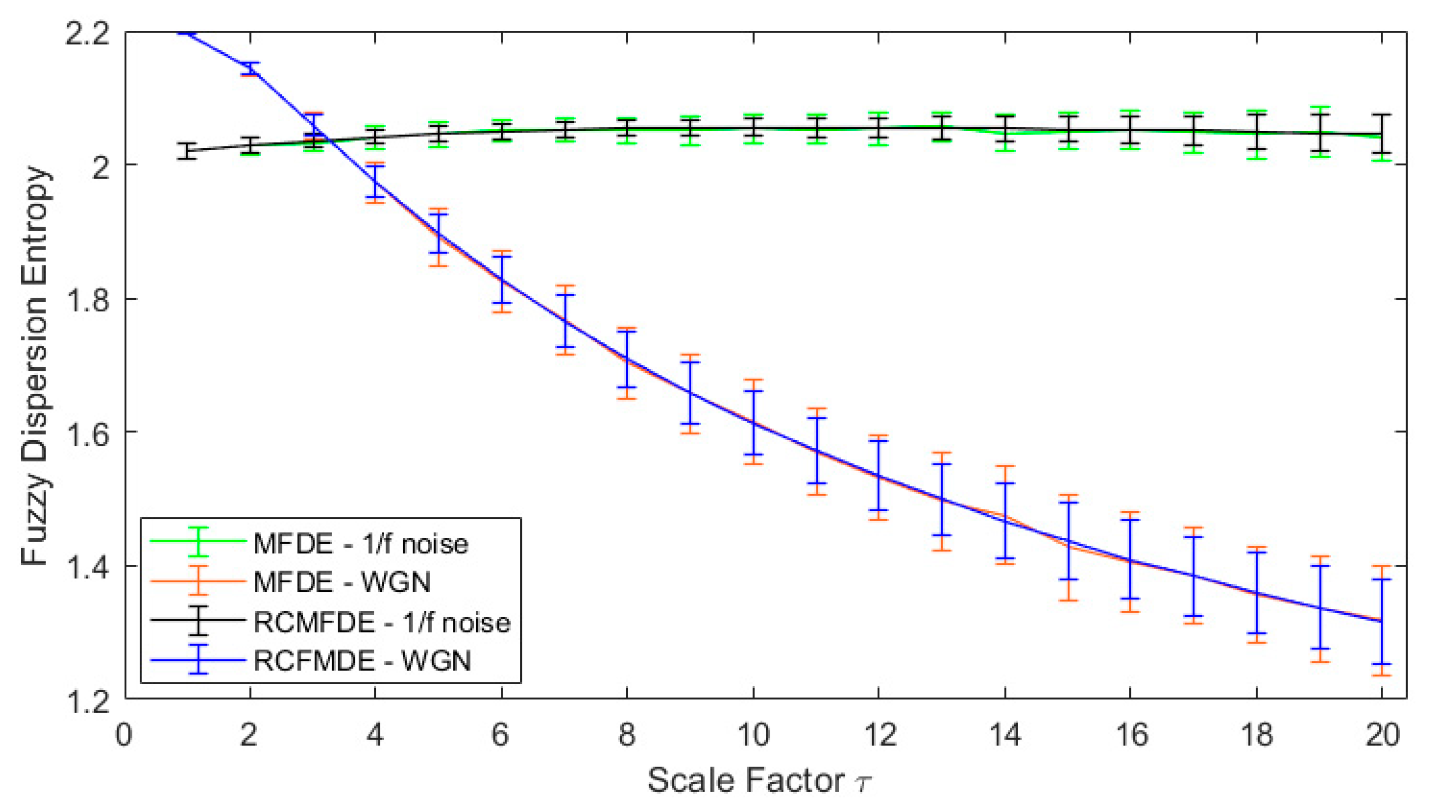
4.1. Analysis of White Gaussian Noise and Noise
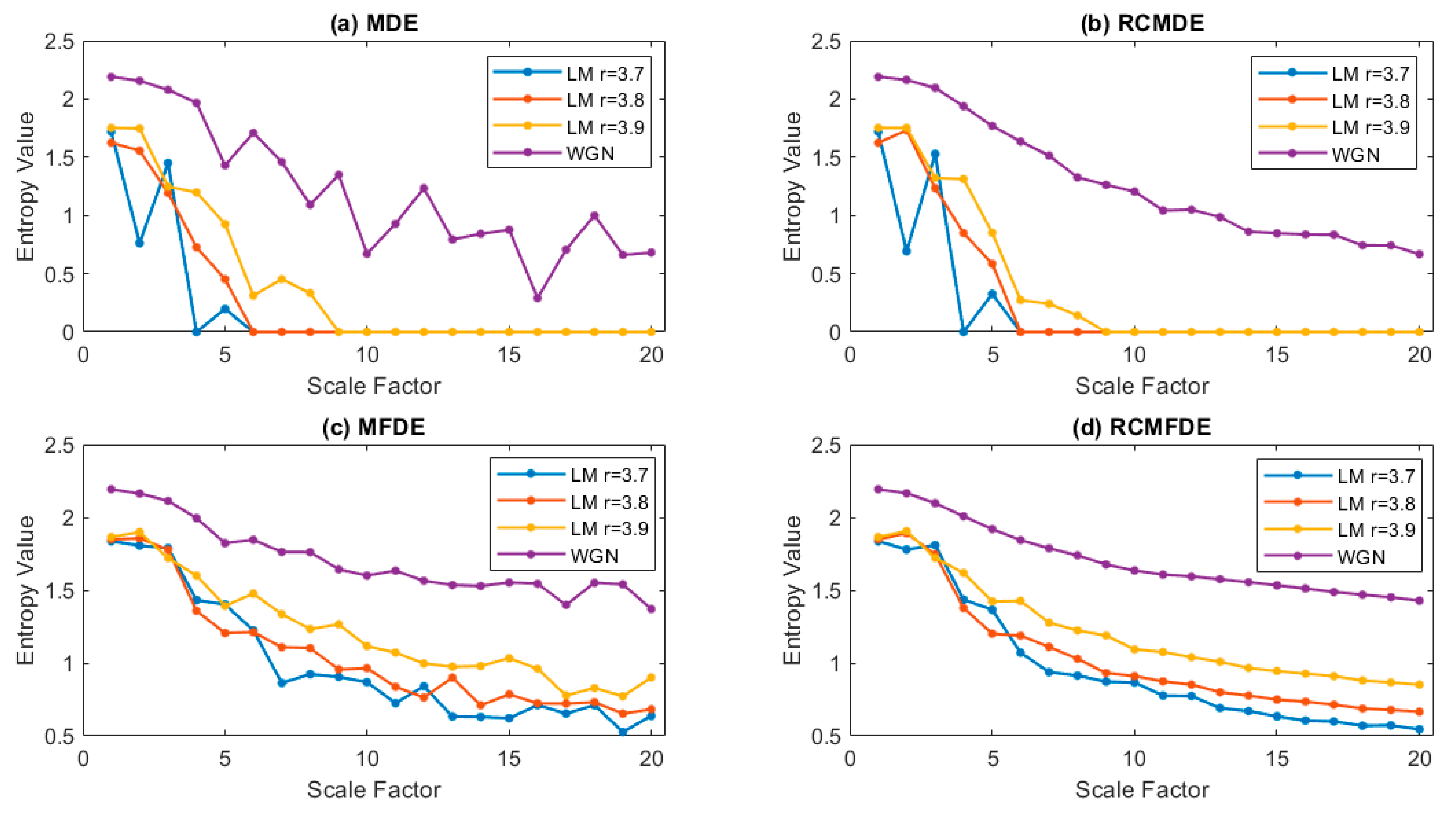
4.2. Analysis of Logistic Map
4.3. Analysis of Chirp signals and Amplitude-Modulated Chirp Signal
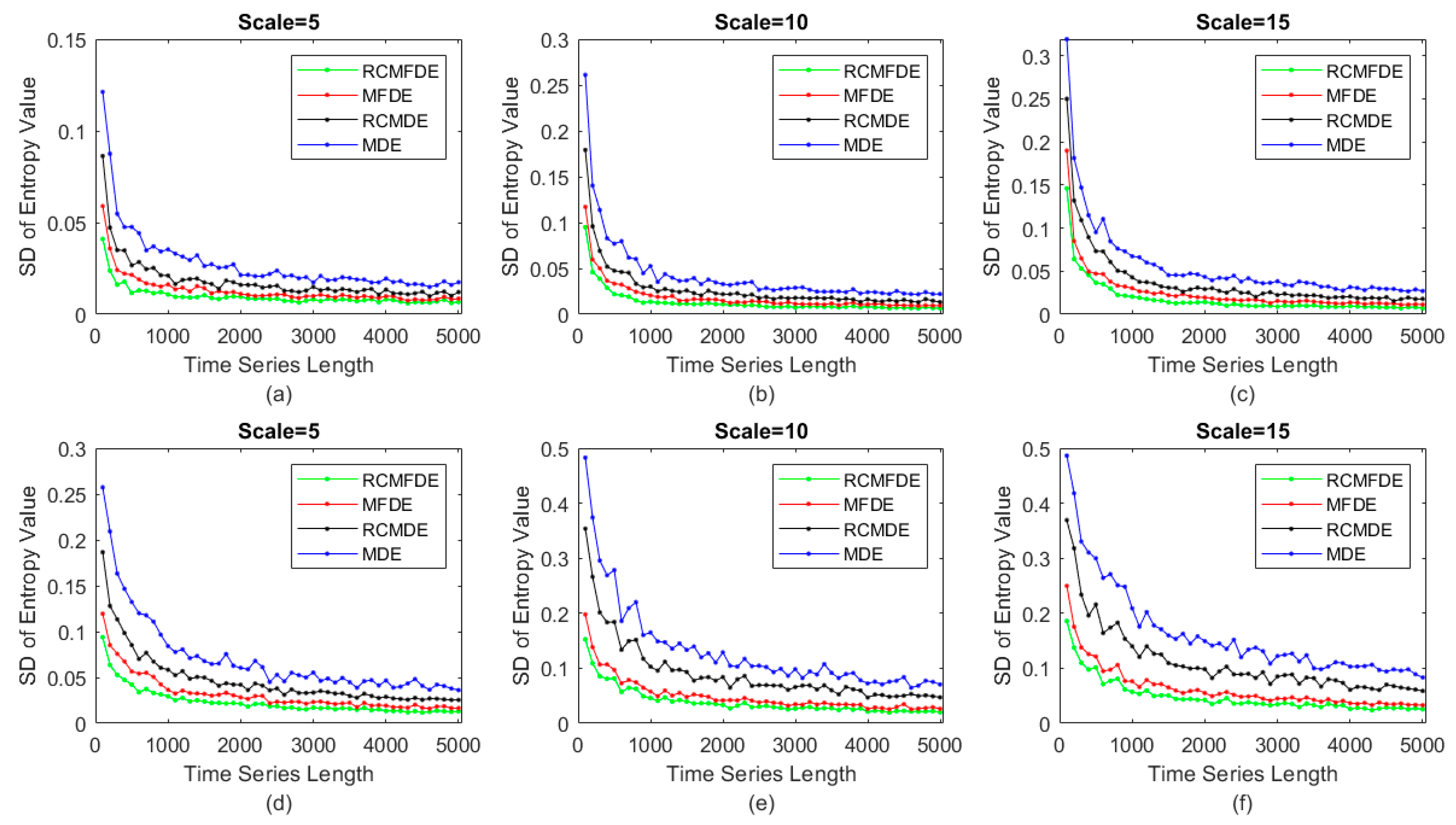
4.4. Sensitivity to Signal Length
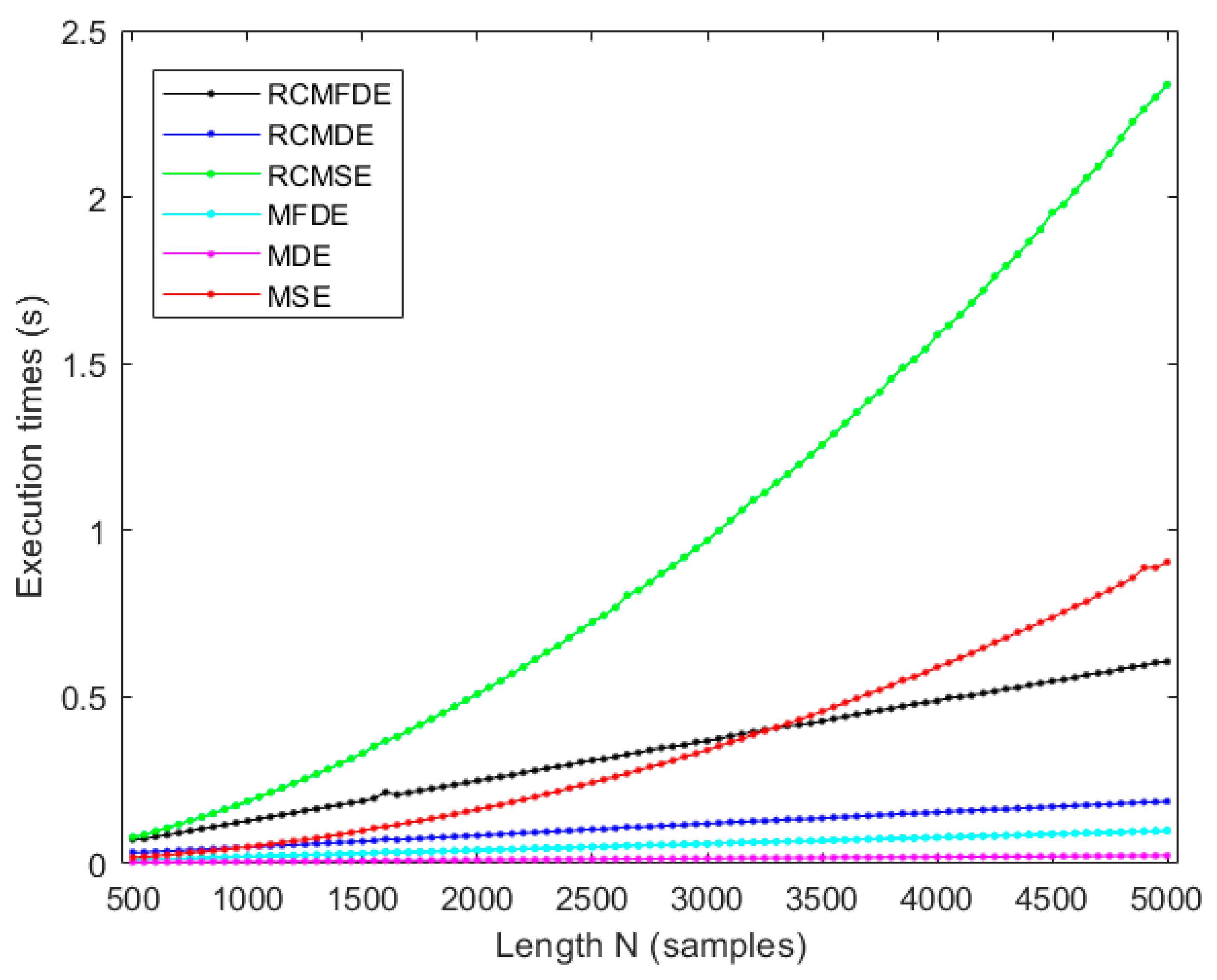
4.5. Computation Time
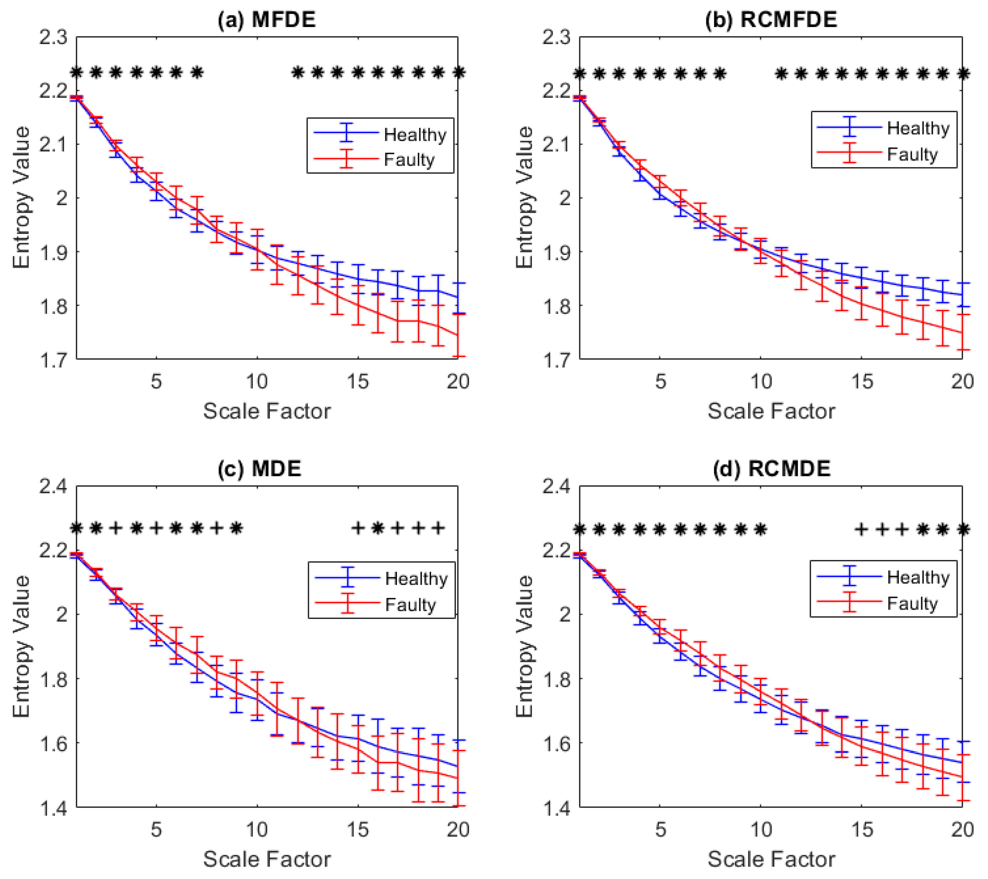
4.6. Simulated Bearing Signal Analysis
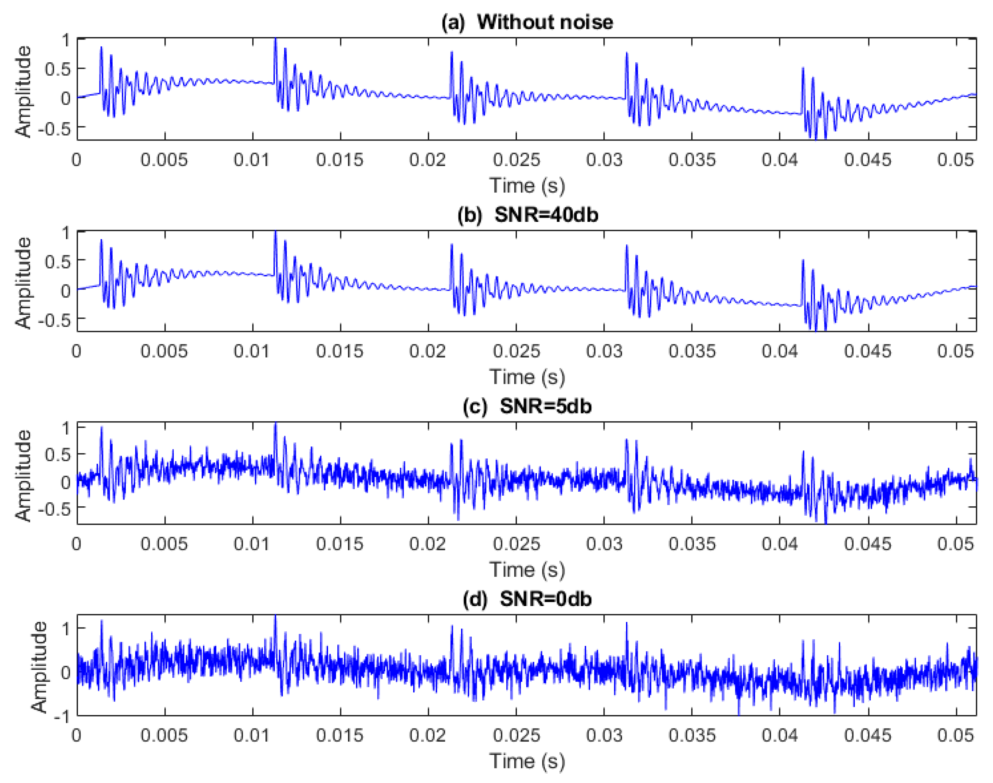
4.7. Noise Effect
4.8. Experimental Data Analysis
4.8.1. Fault Diagnosis with respect to the Paderborn University Bearing Dataset
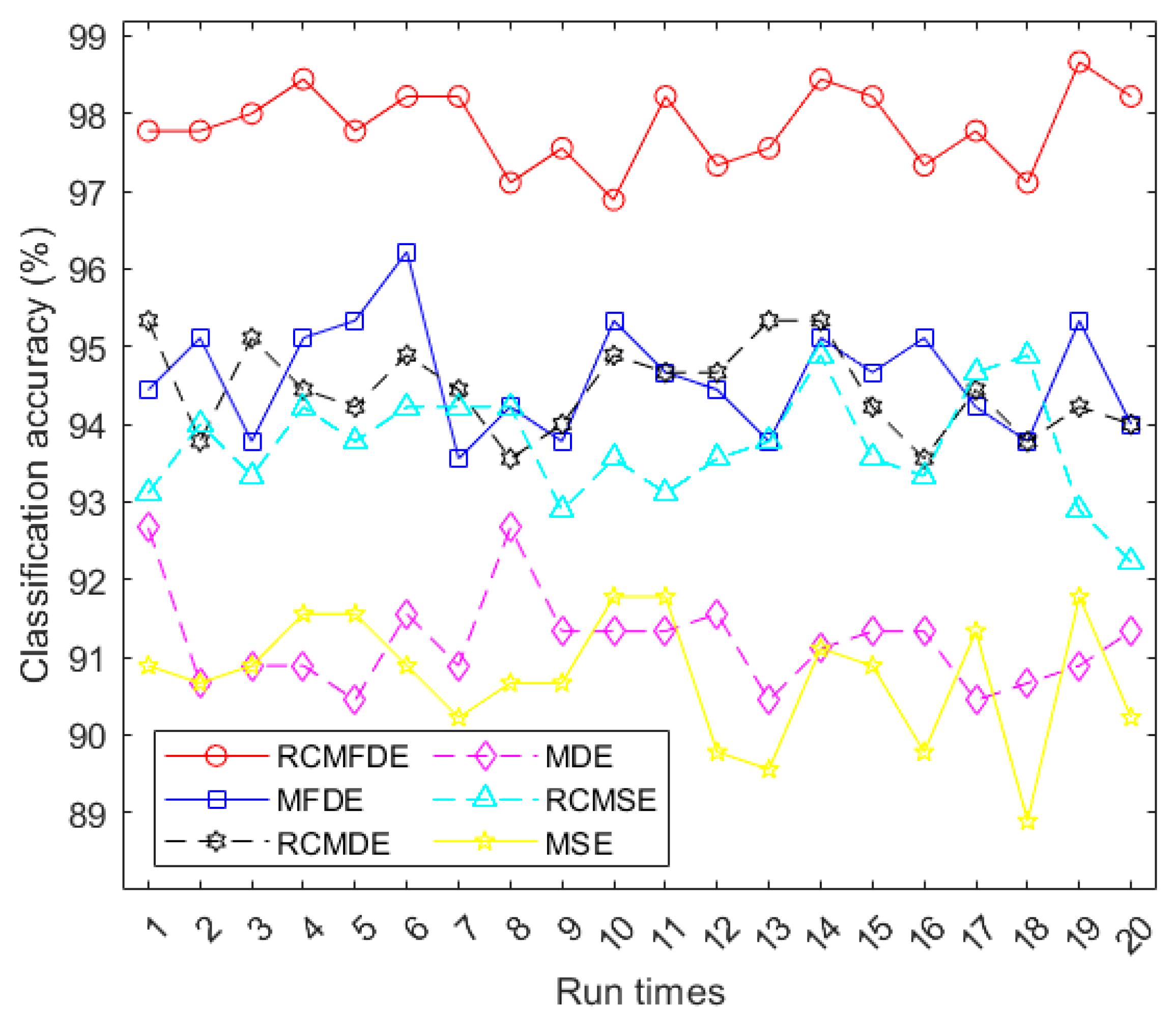
4.8.2. Fault Diagnosis on PHMAP 2021 Data Challenge Dataset
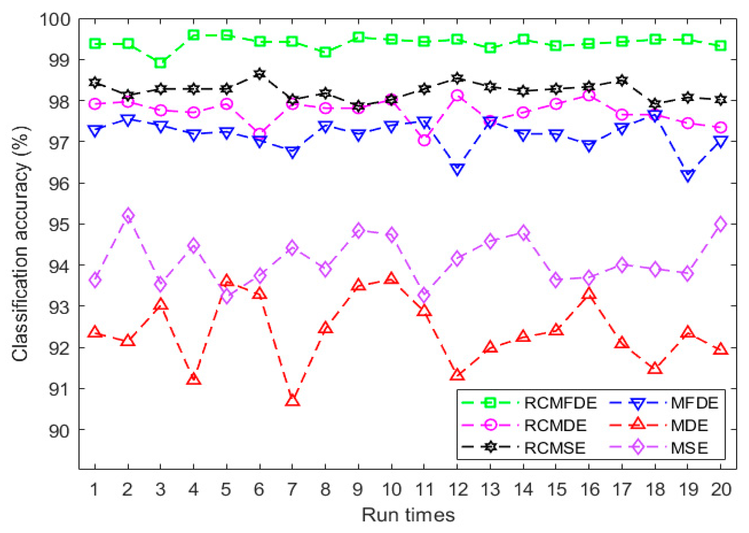
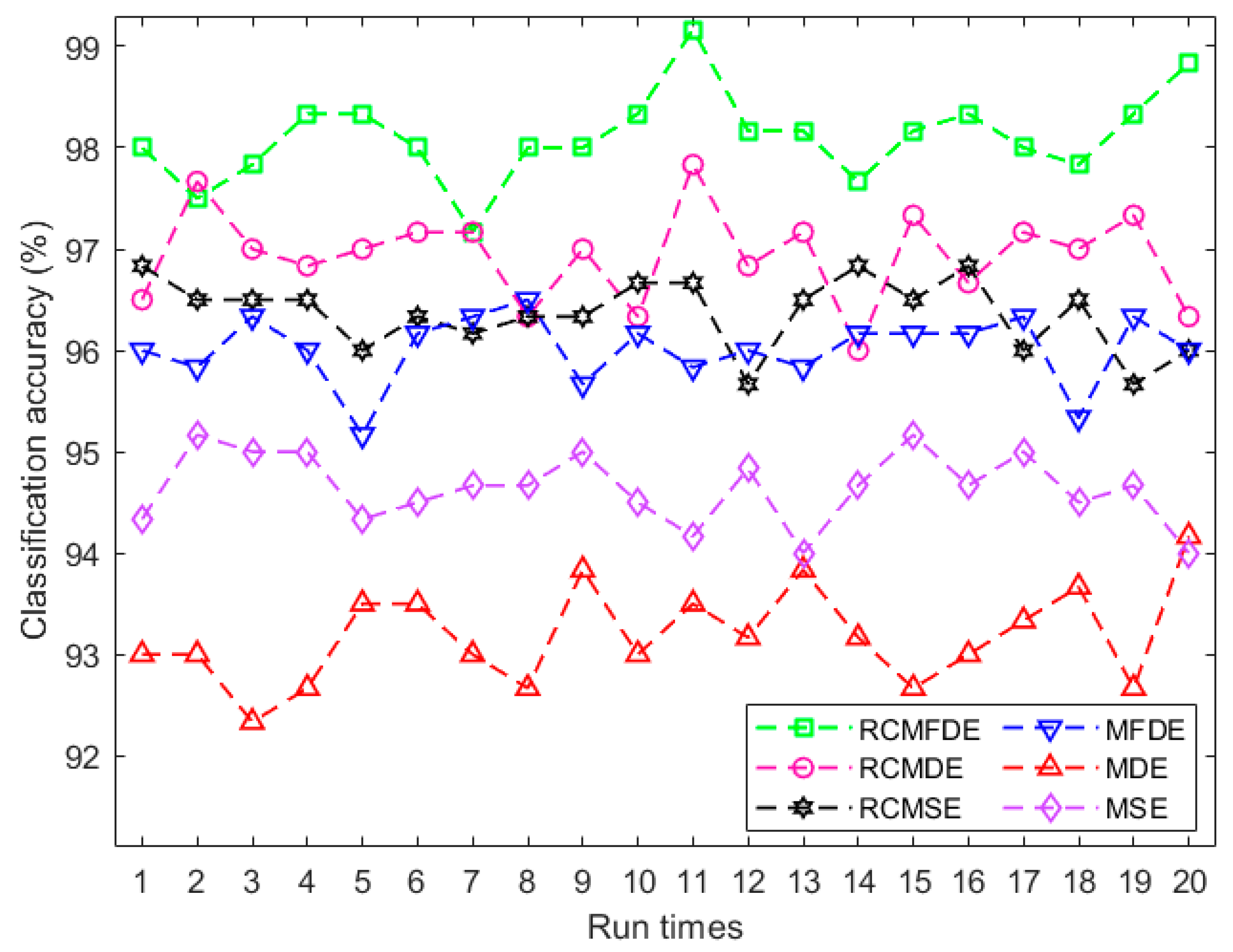
4.8.3. Fault Diagnosis on the Case Western Reserve University (CWRU) Bearing Dataset
5. Conclusions
Author Contributions
Funding
Institutional Review Board Statement
Data Availability Statement
Acknowledgments
Conflicts of Interest
Abbreviations
| CG | Coarse graining |
| CMSE | Composite multiscale sample entropy |
| CWRU | Case Western Reserve University |
| DE | Dispersion entropy |
| DO | Drilling on the outer ring |
| FDE | Fuzzy dispersion entropy |
| FCM-ANFIS | Adaptive neuro-fuzzy inference system with fuzzy c-means |
| FE | Fuzzy entropy |
| H | Healthy condition |
| M. | Multiscale |
| MDE | Multiscale dispersion entropy |
| MFDE | Multiscale fuzzy dispersion entropy |
| MPE | Multiscale permutation entropy |
| MSE | Multiscale sample entropy |
| PE | Permutation entropy |
| PHMAP 2021 | Asia Pacific Conference of the Prognostics and Health Management Society 2021 |
| PO | Pitting on the outer ring |
| RC | Refined composite |
| RCMDE | Refined composite multiscale dispersion entropy |
| RCMFDE | Refined composite multiscale fuzzy dispersion entropy |
| RCMFE | Refined composite multiscale fuzzy entropy |
| RCMPE | Refined composite multiscale permutation entropy |
| RCMSE | Refined composite multiscale sample entropy |
| SE | Sample entropy |
| SD | Standard deviation |
| SNR | Signal-to-noise ratio |
| STO | Sharp trench on the outer ring |
| VMD | Variational mode decomposition |
| WGN | White Gaussian noise |
References
- Yan, X.; Jia, M. Intelligent Fault Diagnosis of Rotating Machinery Using Improved Multiscale Dispersion Entropy and MRMR Feature Selection. Knowl. Based Syst. 2019, 163, 450–471. [Google Scholar] [CrossRef]
- Zhang, L.; Xiong, G.; Liu, H.; Zou, H.; Guo, W. Bearing Fault Diagnosis Using Multi-Scale Entropy and Adaptive Neuro-Fuzzy Inference. Expert Syst. Appl. 2010, 37, 6077–6085. [Google Scholar] [CrossRef]
- Wu, S.-D.; Wu, C.-W.; Wu, T.-Y.; Wang, C.-C. Multi-Scale Analysis Based Ball Bearing Defect Diagnostics Using Mahalanobis Distance and Support Vector Machine. Entropy 2013, 15, 416–433. [Google Scholar] [CrossRef]
- Nandi, S.; Toliyat, H.A.; Li, X. Condition Monitoring and Fault Diagnosis of Electrical Motors—A Review. IEEE Trans. Energy Convers. 2005, 20, 719–729. [Google Scholar] [CrossRef]
- Heng, A.; Zhang, S.; Tan, A.C.C.; Mathew, J. Rotating Machinery Prognostics: State of the Art, Challenges and Opportunities. Mech. Syst. Signal Process. 2009, 23, 724–739. [Google Scholar] [CrossRef]
- Lei, Y.; Lin, J.; He, Z.; Zuo, M.J. A Review on Empirical Mode Decomposition in Fault Diagnosis of Rotating Machinery. Mech. Syst. Signal Process. 2013, 35, 108–126. [Google Scholar] [CrossRef]
- Rostaghi, M.; Reza, M.; Azami, H. Application of Dispersion Entropy to Status Characterization of Rotary Machines. J. Sound Vib. 2019, 438, 291–308. [Google Scholar] [CrossRef]
- Rostaghi, M.; Khatibi, M.M.; Ashory, M.R.; Azami, H. Bearing Fault Diagnosis Using Refined Composite Generalized Multiscale Dispersion Entropy-Based Skewness and Variance and Multiclass FCM-ANFIS. Entropy 2021, 23, 1510. [Google Scholar] [CrossRef]
- Tian, Y.; Wang, Z.; Lu, C. Self-Adaptive Bearing Fault Diagnosis Based on Permutation Entropy and Manifold-Based Dynamic Time Warping. Mech. Syst. Signal Process. 2019, 114, 658–673. [Google Scholar] [CrossRef]
- Li, Y.; Wang, X.; Liu, Z.; Liang, X.; Si, S.; Member, S. The Entropy Algorithm and Its Variants in the Fault Diagnosis of Rotating Machinery: A Review. IEEE Access 2018, 6, 66723–66741. [Google Scholar] [CrossRef]
- Singh, A.; Kankar, P.K.; Kumar, N.; Singh, S. Bearing Fault Detection and Recognition Methodology Based on Weighted Multiscale Entropy Approach. Mech. Syst. Signal Process. 2021, 147, 107073. [Google Scholar] [CrossRef]
- Kim, S.; An, D.; Choi, J.-H. Diagnostics 101: A Tutorial for Fault Diagnostics of Rolling Element Bearing Using Envelope Analysis in MATLAB. Appl. Sci. 2020, 10, 7302. [Google Scholar] [CrossRef]
- Li, Y.; Xu, M.; Wei, Y.; Huang, W. A New Rolling Bearing Fault Diagnosis Method Based on Multiscale Permutation Entropy and Improved Support Vector Machine Based Binary Tree. Measurement 2016, 77, 80–94. [Google Scholar] [CrossRef]
- Wang, Q.; Xiao, Y.; Wang, S.; Liu, W.; Liu, X. A Method for Constructing Automatic Rolling Bearing Fault Identification Model Based on Refined Composite Multi-Scale Dispersion Entropy. IEEE Access 2021, 9, 86412–86428. [Google Scholar] [CrossRef]
- Zheng, J.; Pan, H.; Cheng, J. Rolling Bearing Fault Detection and Diagnosis Based on Composite Multiscale Fuzzy Entropy and Ensemble Support Vector Machines. Mech. Syst. Signal Process. 2017, 85, 746–759. [Google Scholar] [CrossRef]
- Rostaghi, M.; Azami, H. Dispersion Entropy: A Measure for Time-Series Analysis. IEEE Signal Process. Lett. 2016, 23, 610–614. [Google Scholar] [CrossRef]
- Richman, J.S.; Moorman, J.R. Physiological Time-Series Analysis Using Approximate Entropy and Sample Entropy. Am. J. Physiol. Circ. Physiol. 2000, 278, H2039–H2049. [Google Scholar] [CrossRef]
- Azami, H.; Escudero, J. Amplitude- and Fluctuation-Based Dispersion Entropy. Entropy 2018, 20, 210. [Google Scholar] [CrossRef]
- Rostaghi, M.; Khatibi, M.M.; Ashory, M.R.; Azami, H. Fuzzy Dispersion Entropy: A Nonlinear Measure for Signal Analysis. IEEE Trans. Fuzzy Syst. 2021, 30, 3785–3796. [Google Scholar] [CrossRef]
- Ni, Q.; Feng, K.; Wang, K.; Yang, B.; Wang, Y. A Case Study of Sample Entropy Analysis to the Fault Detection of Bearing in Wind Turbine. Case Stud. Eng. Fail. Anal. 2017, 9, 99–111. [Google Scholar] [CrossRef]
- Alcaraz, R.; Abásolo, D.; Hornero, R.; Rieta, J.J. Optimal Parameters Study for Sample Entropy-Based Atrial Fibrillation Organization Analysis. Comput. Methods Programs Biomed. 2010, 99, 124–132. [Google Scholar] [CrossRef] [PubMed]
- Lin, T.-K.; Liang, J.-C. Application of Multi-Scale (Cross-) Sample Entropy for Structural Health Monitoring. Smart Mater. Struct. 2015, 24, 85003. [Google Scholar] [CrossRef]
- Chen, W.; Wang, Z.; Xie, H.; Yu, W. Characterization of Surface EMG Signal Based on Fuzzy Entropy. IEEE Trans. Neural Syst. Rehabil. Eng. 2007, 15, 266–272. [Google Scholar] [CrossRef] [PubMed]
- Noman, K.; Li, Y.; Wen, G.; Patwari, A.U.; Wang, S. Continuous Monitoring of Rolling Element Bearing Health by Nonlinear Weighted Squared Envelope-Based Fuzzy Entropy. Struct. Health Monit. 2023, 14759217231163090. [Google Scholar] [CrossRef]
- Azami, H.; Li, P.; Arnold, S.E.; Escudero, J.; Humeau-Heurtier, A. Fuzzy Entropy Metrics for the Analysis of Biomedical Signals: Assessment and Comparison. IEEE Access 2019, 7, 104833–104847. [Google Scholar] [CrossRef]
- Bandt, C.; Pompe, B. Permutation Entropy: A Natural Complexity Measure for Time Series. Phys. Rev. Lett. 2002, 88, 174102. [Google Scholar] [CrossRef] [PubMed]
- Zanin, M.; Zunino, L.; Rosso, O.A.; Papo, D. Permutation Entropy and Its Main Biomedical and Econophysics Applications: A Review. Entropy 2012, 14, 1553–1577. [Google Scholar] [CrossRef]
- Vashishtha, G.; Chauhan, S.; Singh, M.; Kumar, R. Bearing Defect Identification by Swarm Decomposition Considering Permutation Entropy Measure and Opposition-Based Slime Mould Algorithm. Measurement 2021, 178, 109389. [Google Scholar] [CrossRef]
- Şeker, M.; Özbek, Y.; Yener, G.; Özerdem, M.S. Complexity of EEG Dynamics for Early Diagnosis of Alzheimer’s Disease Using Permutation Entropy Neuromarker. Comput. Methods Programs Biomed. 2021, 206, 106116. [Google Scholar] [CrossRef]
- Zunino, L.; Zanin, M.; Tabak, B.M.; Pérez, D.G.; Rosso, O.A. Forbidden Patterns, Permutation Entropy and Stock Market Inefficiency. Phys. A Stat. Mech. Its Appl. 2009, 388, 2854–2864. [Google Scholar] [CrossRef]
- Consolini, G.; De Michelis, P. Permutation Entropy Analysis of Complex Magnetospheric Dynamics. J. Atmos. Solar-Terr. Phys. 2014, 115, 25–31. [Google Scholar] [CrossRef]
- Kang, Y.; Cai, H.; Song, S. Study and Application of Complexity Model for Hydrological System. Shuili Fadian Xuebao (J. Hydroelectr. Eng.) 2013, 32, 5–10. [Google Scholar]
- Azami, H.; Rostaghi, M.; Abásolo, D.; Escudero, J. Refined Composite Multiscale Dispersion Entropy and Its Application to Biomedical Signals. IEEE Trans. Biomed. Eng. 2017, 64, 2872–2879. [Google Scholar] [PubMed]
- Azami, H.; Rostaghi, M.; Fernandez, A.; Escudero, J. Dispersion Entropy for the Analysis of Resting-State MEG Regularity in Alzheimer’s Disease. In Proceedings of the 2016 38th Annual International Conference of the IEEE Engineering in Medicine and Biology Society (EMBC), Orlando, FL, USA, 16–20 August 2016; pp. 6417–6420. [Google Scholar] [CrossRef]
- Li, S.; Shang, P. Characterizing Nonlinear Time Series via Sliding-Window Amplitude-Based Dispersion Entropy. Fluct. Noise Lett. 2023, 22, 2350023. [Google Scholar] [CrossRef]
- Costa, M.; Goldberger, A.L.; Peng, C.-K. Multiscale Entropy Analysis of Complex Physiologic Time Series. Phys. Rev. Lett. 2002, 89, 68102. [Google Scholar] [CrossRef]
- Aziz, W.; Arif, M. Multiscale Permutation Entropy of Physiological Time Series. In Proceedings of the 2005 Pakistan Section Multitopic Conference, Karachi, Pakistan, 24–25 December 2005. [Google Scholar] [CrossRef]
- Zheng, J.; Cheng, J.; Yang, Y.; Luo, S. A Rolling Bearing Fault Diagnosis Method Based on Multi-Scale Fuzzy Entropy and Variable Predictive Model-Based Class Discrimination. Mech. Mach. Theory 2014, 78, 187–200. [Google Scholar] [CrossRef]
- Wu, S.; Wu, C.; Lee, K.; Lin, S. Modified Multiscale Entropy for Short-Term Time Series Analysis. Phys. A 2013, 392, 5865–5873. [Google Scholar] [CrossRef]
- Wu, S.-D.; Wu, C.-W.; Lin, S.-G.; Wang, C.-C.; Lee, K.-Y. Time Series Analysis Using Composite Multiscale Entropy. Entropy 2013, 15, 1069–1084. [Google Scholar] [CrossRef]
- Wu, S.; Wu, C.; Lin, S.; Lee, K.; Peng, C. Analysis of Complex Time Series Using Refined Composite Multiscale Entropy. Phys. Lett. A 2014, 378, 1369–1374. [Google Scholar] [CrossRef]
- Azami, H.; Fernández, A.; Escudero, J. Refined Multiscale Fuzzy Entropy Based on Standard Deviation for Biomedical Signal Analysis. Med. Biol. Eng. Comput. 2017, 55, 2037–2052. [Google Scholar] [CrossRef]
- Humeau-Heurtier, A.; Wu, C.-W.; Wu, S.-D. Refined Composite Multiscale Permutation Entropy to Overcome Multiscale Permutation Entropy Length Dependence. IEEE Signal Process. Lett. 2015, 22, 2364–2367. [Google Scholar] [CrossRef]
- Wang, Z.; Zheng, L.; Wang, J.; Du, W. Research on Novel Bearing Fault Diagnosis Method Based on Improved Krill Herd Algorithm and Kernel Extreme Learning Machine. Complexity 2019, 2019, 4031795. [Google Scholar] [CrossRef]
- Li, C.; Zheng, J.; Pan, H.; Liu, Q. Fault Diagnosis Method of Rolling Bearings Based on Refined Composite Multiscale Dispersion Entropy and Support Vector Machine. China Mech. Eng. 2019, 30, 1713. [Google Scholar]
- Zhang, X.; Zhao, J.; Teng, H.; Liu, G. A Novel Faults Detection Method for Rolling Bearing Based on RCMDE and ISVM. J. Vibroengineering 2019, 21, 2148–2158. [Google Scholar] [CrossRef]
- Luo, H.; He, C.; Zhou, J.; Zhang, L. Rolling Bearing Sub-Health Recognition via Extreme Learning Machine Based on Deep Belief Network Optimized by Improved Fireworks. IEEE Access 2021, 9, 42013–42026. [Google Scholar] [CrossRef]
- Zhang, W.; Zhou, J. A Comprehensive Fault Diagnosis Method for Rolling Bearings Based on Refined Composite Multiscale Dispersion Entropy and Fast Ensemble Empirical Mode Decomposition. Entropy 2019, 21, 680. [Google Scholar] [CrossRef] [PubMed]
- Luo, S.; Yang, W.; Luo, Y. Fault Diagnosis of a Rolling Bearing Based on Adaptive Sparest Narrow-Band Decomposition and Refined Composite Multiscale Dispersion Entropy. Entropy 2020, 22, 375. [Google Scholar] [CrossRef] [PubMed]
- Zheng, J.; Huang, S.; Pan, H.; Jiang, K. An Improved Empirical Wavelet Transform and Refined Composite Multiscale Dispersion Entropy-Based Fault Diagnosis Method for Rolling Bearing. IEEE Access 2020, 8, 168732–168742. [Google Scholar] [CrossRef]
- Cai, J.; Yang, L.; Zeng, C.; Chen, Y. Integrated Approach for Ball Mill Load Forecasting Based on Improved EWT, Refined Composite Multi-Scale Dispersion Entropy and Fireworks Algorithm Optimized SVM. Adv. Mech. Eng. 2021, 13, 1687814021991264. [Google Scholar] [CrossRef]
- Lv, J.; Sun, W.; Wang, H.; Zhang, F. Coordinated Approach Fusing RCMDE and Sparrow Search Algorithm-Based SVM for Fault Diagnosis of Rolling Bearings. Sensors 2021, 21, 5297. [Google Scholar] [CrossRef]
- Baranwal, G.; Vidyarthi, D.P. Admission Control in Cloud Computing Using Game Theory. J. Supercomput. 2016, 72, 317–346. [Google Scholar] [CrossRef]
- Data Challenge at PHMAP 2021. Available online: http://phmap.org/data-challenge/ (accessed on 18 June 2021).
- Duch, W. Uncertainty of Data, Fuzzy Membership Functions, and Multilayer Perceptrons. IEEE Trans. Neural Netw. 2005, 16, 10–23. [Google Scholar] [CrossRef] [PubMed]
- Costa, M.; Goldberger, A.L.; Peng, C.K. Multiscale Entropy Analysis of Biological Signals. Phys. Rev. E Stat. Nonlinear Soft Matter Phys. 2005, 71, 021906. [Google Scholar] [CrossRef] [PubMed]
- Azami, H.; Arnold, S.E.; Sanei, S.; Chang, Z.; Sapiro, G.; Escudero, J.; Gupta, A.S. Multiscale Fluctuation-Based Dispersion Entropy and Its Applications to Neurological Diseases. IEEE Access 2019, 7, 68718–68733. [Google Scholar] [CrossRef]
- Humeau-Heurtier, A.; Wu, C.-W.; Wu, S.-D.; Mahé, G.; Abraham, P. Refined Multiscale Hilbert–Huang Spectral Entropy and Its Application to Central and Peripheral Cardiovascular Data. IEEE Trans. Biomed. Eng. 2016, 63, 2405–2415. [Google Scholar] [CrossRef] [PubMed]
- Tahmina Akter, M. Observation of Different Behaviors of Logistic Map for Different Control Parameters. Int. J. Appl. Math. Theor. Phys. 2018, 4, 84. [Google Scholar] [CrossRef]
- Wu, S.D.; Wu, C.W.; Humeau-Heurtier, A. Refined Scale-Dependent Permutation Entropy to Analyze Systems Complexity. Phys. A Stat. Mech. Its Appl. 2016, 450, 454–461. [Google Scholar] [CrossRef]
- Yan, R.; Liu, Y.; Gao, R.X. Permutation Entropy: A Nonlinear Statistical Measure for Status Characterization of Rotary Machines. Mech. Syst. Signal Process. 2012, 29, 474–484. [Google Scholar] [CrossRef]
- Rani, M.; Agarwal, R. A New Experimental Approach to Study the Stability of Logistic Map. Chaos Solitons Fractals 2009, 41, 2062–2066. [Google Scholar] [CrossRef]
- Traversaro, F.; Legnani, W.; Redelico, F.O. Influence of the Signal to Noise Ratio for the Estimation of Permutation Entropy. Phys. A 2020, 553, 124134. [Google Scholar] [CrossRef]
- Tian, X.; Xi, J.; Rehab, I.; Abdalla, G.M.; Gu, F.; Ball, A.D. A Robust Detector for Rolling Element Bearing Condition Monitoring Based on the Modulation Signal Bispectrum and Its Performance Evaluation against the Kurtogram. Mech. Syst. Signal Process. 2018, 100, 167–187. [Google Scholar] [CrossRef]
- Zhao, Z.; Qiao, B.; Wang, S.; Shen, Z.; Chen, X. A Weighted Multi-Scale Dictionary Learning Model and Its Applications on Bearing Fault Diagnosis. J. Sound Vib. 2019, 446, 429–452. [Google Scholar] [CrossRef]
- Kedadouche, M.; Liu, Z.; Vu, V.-H. A New Approach Based on OMA-Empirical Wavelet Transforms for Bearing Fault Diagnosis. Measurement 2016, 90, 292–308. [Google Scholar] [CrossRef]
- Lessmeier, C.; Kimotho, J.K.; Zimmer, D.; Sextro, W.; KAt-Data Center, Chair of Design and Drive Technology. Paderborn University. Available online: https://mb.uni-paderborn.de/kat/forschung/datacenter/bearing-datacenter/ (accessed on 14 January 2021).
- Lessmeier, C.; Kimotho, J.K.; Zimmer, D.; Sextro, W. Condition Monitoring of Bearing Damage in Electromechanical Drive Systems by Using Motor Current Signals of Electric Motors: A Benchmark Data Set for Data-Driven Classification. In Proceedings of the PHM Society European Conference, Bilbao, Spain, 5–8 July 2016; Volume 3. [Google Scholar]
- Bearings Vibration Data Set. Case Western Reserve University. Available online: https://csegroups.case.edu/bearingdatacenter/pages/download-data-file (accessed on 23 June 2020).
- Smith, W.A.; Randall, R.B. Rolling Element Bearing Diagnostics Using the Case Western Reserve University Data: A Benchmark Study. Mech. Syst. Signal Process. 2015, 64–65, 100–131. [Google Scholar] [CrossRef]
- Fogedby, H.C. On the Phase Space Approach to Complexity. J. Stat. Phys. 1992, 69, 411–425. [Google Scholar] [CrossRef]
- Jiang, Y.; Mao, D.; Xu, Y. A Fast Algorithm for Computing Sample Entropy. Adv. Adapt. Data Anal. 2011, 3, 167–186. [Google Scholar] [CrossRef]
- Sheen, Y.T. A Complex Filter for Vibration Signal Demodulation in Bearing Defect Diagnosis. J. Sound Vib. 2004, 276, 105–119. [Google Scholar] [CrossRef]
- Rosenthal, R. Parametric Measures of Effect Size in The Handbook of Research Synthesis; Cooper, H., Hedges, L.V., Eds.; Sage: New York, NY, USA, 1994; pp. 231–244. [Google Scholar]


| Methods | Advantages | Disadvantages | Some of Applications |
|---|---|---|---|
| SE | SE deals with the self-matching problem of approximate entropy and eliminates the bias in approximate entropy algorithm [17]. | (1) SE may result in undefined or unreliable entropy values, especially for short time series [18]; (2) SE has high computational cost [19]. | Mechanical [20], biomedical [21], civil engineering [22] |
| FE | FE, compared with SE, leads to more stable and accurate results [23]. | (1) FE may result in undefined or unreliable entropy values, especially for short time series [19]. (2) Computational cost of FE is higher than SE [19]. | Mechanical [24], biomedical [25], |
| PE | (1) PE is faster than SE and FE [16,26]; (2) PE value is more reliable than that for SE or FE for short signals [19]. | (1) PE only captures order relations between amplitude values and ignores some signal information [18,27]; (2) PE neglects equal values in a signal; (3) PE is sensitive to a high SNR noise [18,27]. | Mechanical [28], biomedical [29], economy [30], geophysics [31], hydrology [32] |
| DE | (1) Unlike SE, DE does not lead to undefined results in short signals [33]; (2) DE is less susceptible to the effects of noise [7]; (3) unlike PE, DE considers amplitude values [18]; (4) DE addresses the issue of equal adjacent amplitude values in PE [16]; (5) compared to SE and FE, DE is considerably faster [1,7]. | DE is sensitive to its parameters, particularly the number of classes and embedding dimension [19]. | Mechanical [7], biomedical [34], economy [35] |
| Condition of Bearing | ||||
|---|---|---|---|---|
| H | STO | DO | PO | |
| Bearing Code | K001 | KA01 | KA06 | KA07 |
| No. | Rotational Speed (rpm) | Load Torque (Nm) | Radial Force (N) |
|---|---|---|---|
| 1 | 1500 | 0.7 | 1000 |
| 2 | 1500 | 0.1 | 1000 |
| 3 | 1500 | 0.7 | 400 |
| Feature Extractor | Scale | |||||||||||||||||||
|---|---|---|---|---|---|---|---|---|---|---|---|---|---|---|---|---|---|---|---|---|
| 1 | 2 | 3 | 4 | 5 | 6 | 7 | 8 | 9 | 10 | 11 | 12 | 13 | 14 | 15 | 16 | 17 | 18 | 19 | 20 | |
| RCMFDE | 1.21 | 1.19 | 1.65 | 1.96 | 1.85 | 1.48 | 1.06 | 0.59 | 0.18 | 0.19 | 0.58 | 0.97 | 1.36 | 1.67 | 1.89 | 2.05 | 2.17 | 2.28 | 2.37 | 2.43 |
| MFDE | 1.21 | 0.82 | 0.78 | 1.41 | 1.09 | 0.95 | 0.81 | 0.21 | 0.36 | 0.01 | 0.41 | 0.74 | 0.96 | 1.41 | 1.46 | 1.85 | 2.04 | 1.66 | 1.96 | 2.05 |
| RCMDE | 1.06 | 0.65 | 1.00 | 1.34 | 1.24 | 1.08 | 1.06 | 0.80 | 0.67 | 0.58 | 0.39 | 0.16 | 0.11 | 0.17 | 0.37 | 0.46 | 0.48 | 0.56 | 0.64 | 0.69 |
| MDE | 1.06 | 0.58 | 0.36 | 0.77 | 0.52 | 0.77 | 0.74 | 0.53 | 0.72 | 0.29 | 0.21 | 0.01 | 0.18 | 0.17 | 0.483 | 0.61 | 0.37 | 0.45 | 0.46 | 0.45 |
| WGN | Method | Scale | |||||
|---|---|---|---|---|---|---|---|
| 1 | 2 | 3 | 4 | 5 | |||
| SNR = 40 db | MDE | mean | 1.0016 | 1.0010 | 1.0005 | 0.9987 | 0.9998 |
| SD | 0.0026 | 0.0019 | 0.0028 | 0.0028 | 0.0023 | ||
| RCMDE | mean | 1.0016 | 1.0010 | 1.0000 | 0.9997 | 0.9997 | |
| SD | 0.0026 | 0.0015 | 0.0015 | 0.0013 | 0.0012 | ||
| MFDE | mean | 1.0003 | 1.0001 | 1.0001 | 1.0001 | 1.0000 | |
| SD | 3.2605 × 10⁻⁴ | 2.9003 × 10⁻⁴ | 2.5598 × 10⁻⁴ | 2.4340 × 10⁻⁴ | 2.1888 × 10⁻⁴ | ||
| RCMFDE | mean | 1.0003 | 1.0001 | 1.0001 | 1.0001 | 1.0000 | |
| SD | 3.2605 × 10⁻⁴ | 2.7657 × 10⁻⁴ | 2.3455 × 10⁻⁴ | 2.1962 × 10⁻⁴ | 1.9927 × 10⁻⁴ | ||
| SNR = 5 db | MDE | mean | 1.4262 | 1.2168 | 1.1234 | 1.0792 | 1.056 0 |
| SD | 0.0115 | 0.0138 | 0.0166 | 0.0179 | 0.0215 | ||
| RCMDE | mean | 1.4262 | 1.2142 | 1.1243 | 1.079 0 | 1.0535 | |
| SD | 0.0115 | 0.0127 | 0.0122 | 0.0125 | 0.0125 | ||
| MFDE | mean | 1.2057 | 1.1186 | 1.0756 | 1.0557 | 1.0452 | |
| SD | 0.0055 | 0.0056 | 0.0061 | 0.0067 | 0.0048 | ||
| RCMFDE | mean | 1.2057 | 1.1176 | 1.0767 | 1.0557 | 1.0441 | |
| SD | 0.0055 | 0.0053 | 0.0052 | 0.0049 | 0.0044 | ||
| SNR = 0 db | MDE | mean | 1.5310 | 1.3157 | 1.2028 | 1.1404 | 1.1078 |
| SD | 0.0067 | 0.0093 | 0.0142 | 0.0191 | 0.0183 | ||
| RCMDE | mean | 1.5310 | 1.3165 | 1.2038 | 1.1412 | 1.1069 | |
| SD | 0.0067 | 0.0064 | 0.0081 | 0.0118 | 0.0122 | ||
| MFDE | mean | 1.2741 | 1.1767 | 1.1207 | 1.0877 | 1.0709 | |
| SD | 0.0038 | 0.0046 | 0.0059 | 0.0059 | 0.0075 | ||
| RCMFDE | mean | 1.2741 | 1.1777 | 1.1212 | 1.0883 | 1.0698 | |
| SD | 0.0038 | 0.0030 | 0.0035 | 0.0042 | 0.0048 | ||
| Feature Extractor | Accuracy (%) | ||
|---|---|---|---|
| Min | Mean | Max | |
| RCMFDE | 97.17 | 98.11 | 99.17 |
| RCMDE | 96.00 | 96.93 | 97.83 |
| RCMSE | 95.67 | 96.37 | 96.83 |
| MFDE | 95.17 | 96.02 | 96.50 |
| MDE | 92.33 | 93.18 | 94.17 |
| MSE | 94.00 | 94.64 | 95.17 |
| True Condition | ||||||
|---|---|---|---|---|---|---|
| H | STO | DO | PO | Sensitivity (%) | ||
| Predicted condition | H | 150 | 0 | 1 | 0 | 99.34 |
| STO | 0 | 150 | 0 | 0 | 100 | |
| DO | 0 | 0 | 147 | 2 | 98.66 | |
| PO | 0 | 0 | 2 | 148 | 98.67 | |
| Precision (%) | 100 | 100 | 98 | 98.67 | A * = 99.17 | |
| Features | Accuracy (%) | ||
|---|---|---|---|
| Min | Mean | Max | |
| RCMFDE | 96.89 | 97.83 | 98.67 |
| MFDE | 93.56 | 94.60 | 96.22 |
| RCMDE | 93.56 | 94.444 | 95.33 |
| MDE | 90.44 | 91.19 | 92.67 |
| RCMSE | 92.22 | 93.72 | 94.89 |
| MSE | 88.89 | 90.74 | 91.78 |
| True Condition | |||||
|---|---|---|---|---|---|
| Belt Looseness High | Bearing Fault | Normal | Sensitivity (%) | ||
| Predicted condition | Belt Looseness High | 147 | 0 | 3 | 98 |
| Bearing fault | 2 | 150 | 0 | 98.68 | |
| Normal | 1 | 0 | 147 | 99.32 | |
| Precision (%) | 98 | 100 | 98 | AC * = 98.67 | |
| Bearing Condition | Fault Diameter (mm) | Fault Position Relative to Load Zone | Label of Classification |
|---|---|---|---|
| Normal | 0 | - | 1 |
| Rolling element | 0.1778 | - | 2 |
| Rolling element | 0.3556 | - | 3 |
| Rolling element | 0.5334 | - | 4 |
| Rolling element | 0.7112 | - | 5 |
| Inner race | 0.1778 | - | 6 |
| Inner race | 0.3556 | - | 7 |
| Inner race | 0.5334 | - | 8 |
| Inner race | 0.7112 | - | 9 |
| Outer race | 0.1778 | Centered @ 6:00 | 10 |
| Outer race | 0.3556 | Centered @ 6:00 | 11 |
| Outer race | 0.5334 | Centered @ 6:00 | 12 |
| Outer race | 0.1778 | Orthogonal @ 3:00 | 13 |
| Outer race | 0.5334 | Orthogonal @ 3:00 | 14 |
| Outer race | 0.1778 | Opposite @ 12:00 | 15 |
| Outer race | 0.5334 | Opposite @ 12:00 | 16 |
| Features | Accuracy (%) | ||
|---|---|---|---|
| Min | Mean | Max | |
| RCMFDE | 98.91 | 99.39 | 99.58 |
| RCMDE | 97.03 | 97.73 | 98.12 |
| RCMSE | 97.86 | 98.23 | 98.65 |
| MFDE | 96.20 | 97.17 | 97.66 |
| MDE | 90.68 | 92.38 | 93.65 |
| MSE | 93.23 | 94.13 | 95.21 |
| True Condition | ||||||||||||||||||
|---|---|---|---|---|---|---|---|---|---|---|---|---|---|---|---|---|---|---|
| Class | 1 | 2 | 3 | 4 | 5 | 6 | 7 | 8 | 9 | 10 | 11 | 12 | 13 | 14 | 15 | 16 | Sensitivity | |
| Predicted condition | 1 | 120 | 0 | 0 | 0 | 0 | 0 | 0 | 0 | 0 | 0 | 0 | 0 | 0 | 0 | 0 | 0 | 100 |
| 2 | 0 | 120 | 0 | 2 | 0 | 0 | 0 | 0 | 0 | 0 | 0 | 0 | 0 | 0 | 0 | 0 | 98.36 | |
| 3 | 0 | 0 | 118 | 0 | 0 | 0 | 0 | 0 | 0 | 0 | 0 | 0 | 0 | 0 | 0 | 0 | 100 | |
| 4 | 0 | 0 | 2 | 115 | 0 | 0 | 0 | 0 | 0 | 0 | 0 | 0 | 0 | 0 | 0 | 0 | 98.29 | |
| 5 | 0 | 0 | 0 | 0 | 120 | 0 | 0 | 0 | 0 | 0 | 0 | 0 | 0 | 0 | 0 | 0 | 100 | |
| 6 | 0 | 0 | 0 | 0 | 0 | 120 | 0 | 0 | 0 | 0 | 1 | 0 | 0 | 0 | 0 | 0 | 99.17 | |
| 7 | 0 | 0 | 0 | 1 | 0 | 0 | 120 | 0 | 0 | 0 | 0 | 0 | 0 | 0 | 0 | 0 | 99.17 | |
| 8 | 0 | 0 | 0 | 0 | 0 | 0 | 0 | 120 | 0 | 0 | 0 | 0 | 0 | 0 | 0 | 0 | 100 | |
| 9 | 0 | 0 | 0 | 0 | 0 | 0 | 0 | 0 | 120 | 0 | 0 | 0 | 0 | 0 | 0 | 0 | 100 | |
| 10 | 0 | 0 | 0 | 0 | 0 | 0 | 0 | 0 | 0 | 120 | 0 | 0 | 0 | 0 | 0 | 0 | 100 | |
| 11 | 0 | 0 | 0 | 0 | 0 | 0 | 0 | 0 | 0 | 0 | 119 | 0 | 0 | 0 | 0 | 0 | 100 | |
| 12 | 0 | 0 | 0 | 0 | 0 | 0 | 0 | 0 | 0 | 0 | 0 | 120 | 0 | 0 | 0 | 0 | 100 | |
| 13 | 0 | 0 | 0 | 0 | 0 | 0 | 0 | 0 | 0 | 0 | 0 | 0 | 120 | 0 | 0 | 0 | 100 | |
| 14 | 0 | 0 | 0 | 0 | 0 | 0 | 0 | 0 | 0 | 0 | 0 | 0 | 0 | 120 | 0 | 0 | 100 | |
| 15 | 0 | 0 | 0 | 2 | 0 | 0 | 0 | 0 | 0 | 0 | 0 | 0 | 0 | 0 | 120 | 0 | 98.36 | |
| 16 | 0 | 0 | 0 | 0 | 0 | 0 | 0 | 0 | 0 | 0 | 0 | 0 | 0 | 0 | 0 | 120 | 100 | |
| Precision | 100 | 100 | 98.33 | 95.83 | 100 | 100 | 100 | 100 | 100 | 100 | 99.17 | 100 | 100 | 100 | 100 | 100 | A* = 99.58 | |
Disclaimer/Publisher’s Note: The statements, opinions and data contained in all publications are solely those of the individual author(s) and contributor(s) and not of MDPI and/or the editor(s). MDPI and/or the editor(s) disclaim responsibility for any injury to people or property resulting from any ideas, methods, instructions or products referred to in the content. |
© 2023 by the authors. Licensee MDPI, Basel, Switzerland. This article is an open access article distributed under the terms and conditions of the Creative Commons Attribution (CC BY) license (https://creativecommons.org/licenses/by/4.0/).
Share and Cite
Rostaghi, M.; Khatibi, M.M.; Ashory, M.R.; Azami, H. Refined Composite Multiscale Fuzzy Dispersion Entropy and Its Applications to Bearing Fault Diagnosis. Entropy 2023, 25, 1494. https://doi.org/10.3390/e25111494
Rostaghi M, Khatibi MM, Ashory MR, Azami H. Refined Composite Multiscale Fuzzy Dispersion Entropy and Its Applications to Bearing Fault Diagnosis. Entropy. 2023; 25(11):1494. https://doi.org/10.3390/e25111494
Chicago/Turabian StyleRostaghi, Mostafa, Mohammad Mahdi Khatibi, Mohammad Reza Ashory, and Hamed Azami. 2023. "Refined Composite Multiscale Fuzzy Dispersion Entropy and Its Applications to Bearing Fault Diagnosis" Entropy 25, no. 11: 1494. https://doi.org/10.3390/e25111494
APA StyleRostaghi, M., Khatibi, M. M., Ashory, M. R., & Azami, H. (2023). Refined Composite Multiscale Fuzzy Dispersion Entropy and Its Applications to Bearing Fault Diagnosis. Entropy, 25(11), 1494. https://doi.org/10.3390/e25111494