
Quantifying Soil Complexity Using Fisher Shannon Method on 3D X-ray Computed Tomography Scans

 , , ,
, , ,  and
and
Abstract
:1. Introduction
2. Methodology
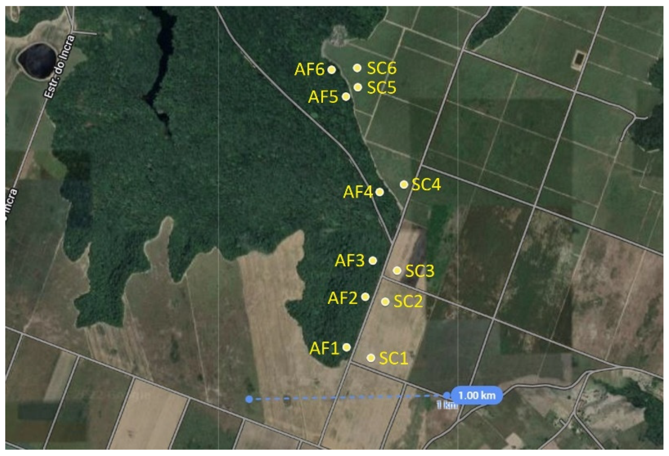
2.1. Soil Samples
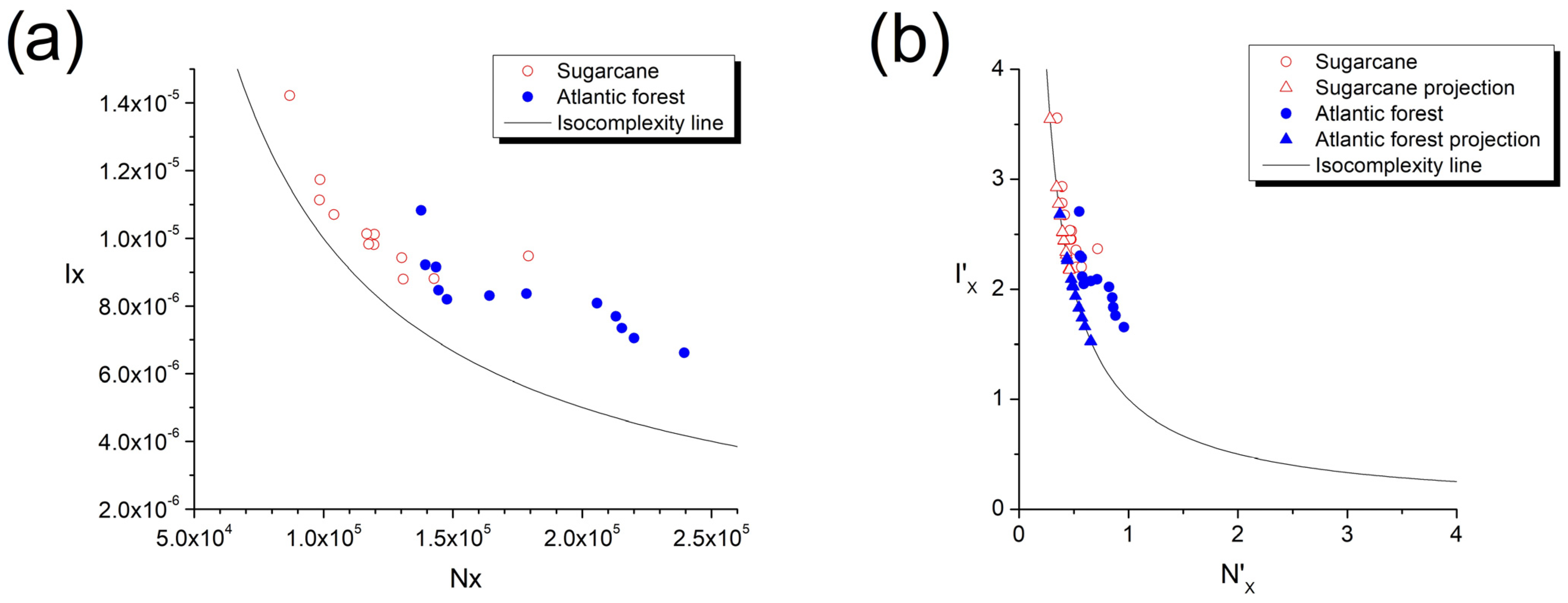
2.2. The Fisher–Shannon Method
3. Results and Discussion
4. Conclusions
Author Contributions
Funding
Institutional Review Board Statement
Data Availability Statement
Acknowledgments
Conflicts of Interest
Appendix A

| Min | Q1 | Q2 | Q3 | Max | Mean | Stdev | |
|---|---|---|---|---|---|---|---|
| Atlantic Forest | |||||||
| AF1-10 | 4.24 × 10⁻⁶ | 6.07 × 10⁻⁶ | 6.50 × 10⁻⁶ | 7.01 × 10⁻⁶ | 1.62 × 10⁻⁵ | 6.62 × 10⁻⁶ | 8.67 × 10⁻⁷ |
| AF2-10 | 3.53 × 10⁻⁶ | 6.79 × 10⁻⁶ | 7.52 × 10⁻⁶ | 8.40 × 10⁻⁶ | 1.76 × 10⁻⁵ | 7.70 × 10⁻⁶ | 1.29 × 10⁻⁶ |
| AF3-10 | 3.65 × 10⁻⁶ | 6.28 × 10⁻⁶ | 6.89 × 10⁻⁶ | 7.64 × 10⁻⁶ | 1.79 × 10⁻⁵ | 7.05 × 10⁻⁶ | 1.09 × 10⁻⁶ |
| AF4-10 | 3.31 × 10⁻⁶ | 6.54 × 10⁻⁶ | 7.14 × 10⁻⁶ | 7.89 × 10⁻⁶ | 1.69 × 10⁻⁵ | 7.34 × 10⁻⁶ | 1.19 × 10⁻⁶ |
| AF5-10 | 4.13 × 10⁻⁶ | 7.13 × 10⁻⁶ | 7.90 × 10⁻⁶ | 8.81 × 10⁻⁶ | 2.02 × 10⁻⁵ | 8.08 × 10⁻⁶ | 1.36 × 10⁻⁶ |
| AF6-10 | 3.79 × 10⁻⁶ | 9.58 × 10⁻⁶ | 1.07 × 10⁻⁵ | 1.19 × 10⁻⁵ | 2.59 × 10⁻⁵ | 1.08 × 10⁻⁵ | 1.86 × 10⁻⁶ |
| AF1-20 | 4.51 × 10⁻⁶ | 7.46 × 10⁻⁶ | 8.14 × 10⁻⁶ | 8.86 × 10⁻⁶ | 1.46 × 10⁻⁵ | 8.20 × 10⁻⁶ | 1.03 × 10⁻⁶ |
| AF2-20 | 3.32 × 10⁻⁶ | 8.10 × 10⁻⁶ | 9.02 × 10⁻⁶ | 1.01 × 10⁻⁵ | 1.78 × 10⁻⁵ | 9.15 × 10⁻⁶ | 1.47 × 10⁻⁶ |
| AF3-20 | 3.45 × 10⁻⁶ | 7.63 × 10⁻⁶ | 8.37 × 10⁻⁶ | 9.20 × 10⁻⁶ | 1.74 × 10⁻⁵ | 8.47 × 10⁻⁶ | 1.19 × 10⁻⁶ |
| AF4-20 | 3.93 × 10⁻⁶ | 7.47 × 10⁻⁶ | 8.20 × 10⁻⁶ | 9.04 × 10⁻⁶ | 1.58 × 10⁻⁵ | 8.31 × 10⁻⁶ | 1.18 × 10⁻⁶ |
| AF5-20 | 3.69 × 10⁻⁶ | 7.33 × 10⁻⁶ | 8.18 × 10⁻⁶ | 9.21 × 10⁻⁶ | 1.82 × 10⁻⁵ | 8.37 × 10⁻⁶ | 1.50 × 10⁻⁶ |
| AF6-20 | 4.08 × 10⁻⁶ | 8.11 × 10⁻⁶ | 9.08 × 10⁻⁶ | 1.02 × 10⁻⁵ | 1.82 × 10⁻⁵ | 9.22 × 10⁻⁶ | 1.54 × 10⁻⁶ |
| Sugarcane | |||||||
| SC1-10 | 4.91 × 10⁻⁶ | 8.15 × 10⁻⁶ | 8.76 × 10⁻⁶ | 9.40 × 10⁻⁶ | 1.45 × 10⁻⁵ | 8.80 × 10⁻⁶ | 9.37 × 10⁻⁷ |
| SC2-10 | 3.24 × 10⁻⁶ | 8.35 × 10⁻⁶ | 9.35 × 10⁻⁶ | 1.05 × 10⁻⁵ | 2.02 × 10⁻⁵ | 9.47 × 10⁻⁶ | 1.60 × 10⁻⁶ |
| SC3-10 | 3.57 × 10⁻⁶ | 9.05 × 10⁻⁶ | 9.78 × 10⁻⁶ | 1.05 × 10⁻⁵ | 1.61 × 10⁻⁵ | 9.81 × 10⁻⁶ | 1.13 × 10⁻⁶ |
| SC4-10 | 4.52 × 10⁻⁶ | 9.02 × 10⁻⁶ | 9.77 × 10⁻⁶ | 1.06 × 10⁻⁵ | 1.71 × 10⁻⁵ | 9.83 × 10⁻⁶ | 1.16 × 10⁻⁶ |
| SC5-10 | 4.01 × 10⁻⁶ | 9.22 × 10⁻⁶ | 1.01 × 10⁻⁵ | 1.10 × 10⁻⁵ | 1.82 × 10⁻⁵ | 1.01 × 10⁻⁵ | 1.31 × 10⁻⁶ |
| SC6-10 | 3.67 × 10⁻⁶ | 1.07 × 10⁻⁵ | 1.17 × 10⁻⁵ | 1.27 × 10⁻⁵ | 1.94 × 10⁻⁵ | 1.17 × 10⁻⁵ | 1.45 × 10⁻⁶ |
| SC1-20 | 5.11 × 10⁻⁶ | 1.03 × 10⁻⁵ | 1.11 × 10⁻⁵ | 1.19 × 10⁻⁵ | 1.72 × 10⁻⁵ | 1.11 × 10⁻⁵ | 1.15 × 10⁻⁶ |
| SC2-20 | 3.51 × 10⁻⁶ | 8.54 × 10⁻⁶ | 9.36 × 10⁻⁶ | 1.02 × 10⁻⁵ | 1.81 × 10⁻⁵ | 9.43 × 10⁻⁶ | 1.30 × 10⁻⁶ |
| SC3-20 | 3.46 × 10⁻⁶ | 9.87 × 10⁻⁶ | 1.07 × 10⁻⁵ | 1.15 × 10⁻⁵ | 1.78 × 10⁻⁵ | 1.07 × 10⁻⁵ | 1.24 × 10⁻⁶ |
| SC4-20 | 3.96 × 10⁻⁶ | 7.93 × 10⁻⁶ | 8.71 × 10⁻⁶ | 9.57 × 10⁻⁶ | 1.72 × 10⁻⁵ | 8.81 × 10⁻⁶ | 1.26 × 10⁻⁶ |
| SC5-20 | 3.71 × 10⁻⁶ | 9.17 × 10⁻⁶ | 1.01 × 10⁻⁵ | 1.11 × 10⁻⁵ | 1.79 × 10⁻⁵ | 1.01 × 10⁻⁵ | 1.43 × 10⁻⁶ |
| SC6-20 | 6.56 × 10⁻⁶ | 1.27 × 10⁻⁵ | 1.41 × 10⁻⁵ | 1.56 × 10⁻⁵ | 2.68 × 10⁻⁵ | 1.42 × 10⁻⁵ | 2.17 × 10⁻⁶ |
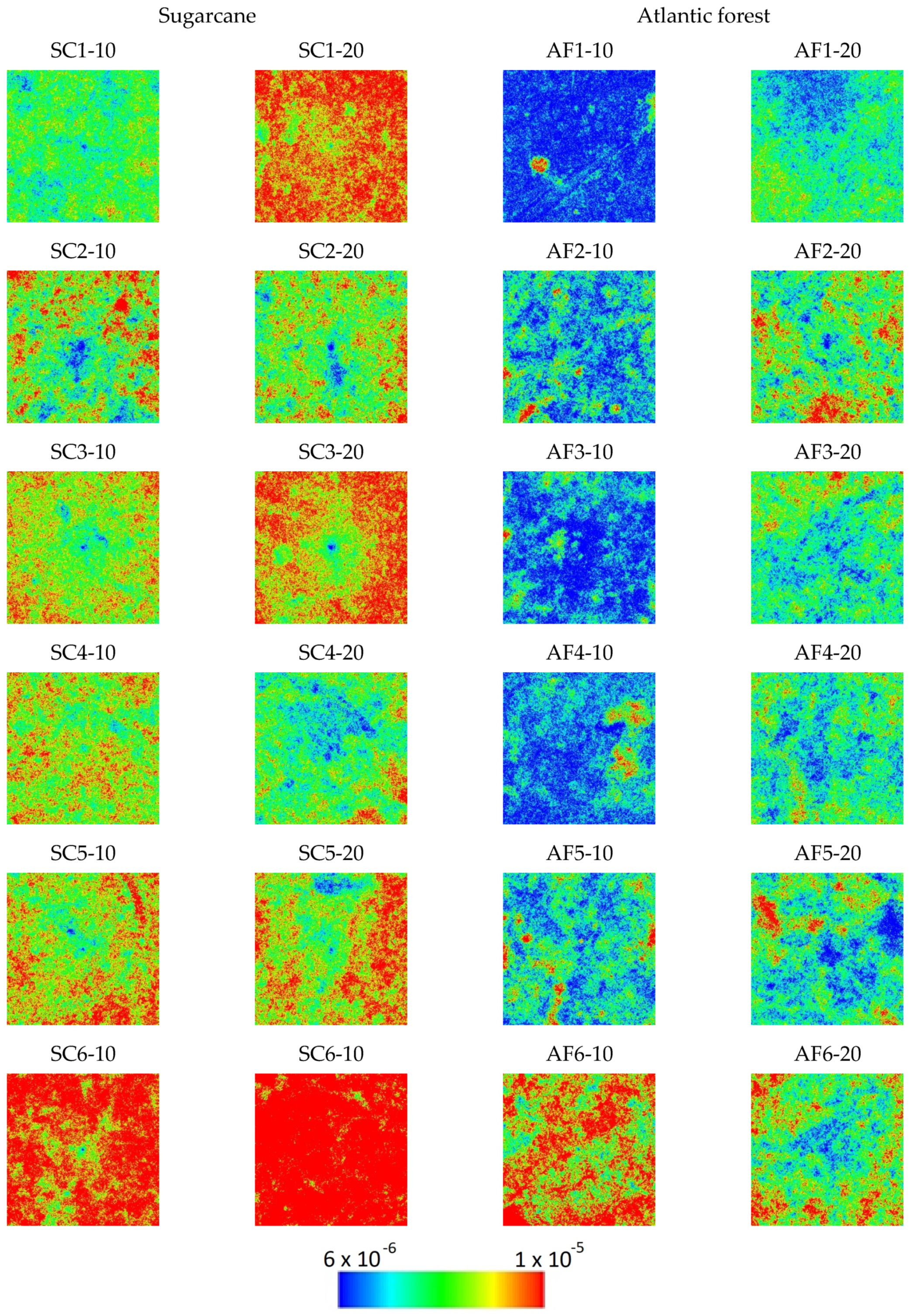
| Min | Q1 | Q2 | Q3 | Max | Mean | Stdev | |
|---|---|---|---|---|---|---|---|
| Atlantic Forest | |||||||
| AF1-10 | 1.24 × 10⁵ | 2.14 × 10⁵ | 2.37 × 10⁵ | 2.62 × 10⁵ | 4.10 × 10⁵ | 2.39 × 10⁵ | 3.53 × 10⁴ |
| AF2-10 | 7.07 × 10⁴ | 1.84 × 10⁵ | 2.11 × 10⁵ | 2.39 × 10⁵ | 6.14 × 10⁵ | 2.13 × 10⁵ | 4.03 × 10⁴ |
| AF3-10 | 7.43 × 10⁴ | 1.92 × 10⁵ | 2.17 × 10⁵ | 2.44 × 10⁵ | 6.00 × 10⁵ | 2.20 × 10⁵ | 3.99 × 10⁴ |
| AF4-10 | 9.73 × 10⁴ | 1.85 × 10⁵ | 2.09 × 10⁵ | 2.37 × 10⁵ | 6.23 × 10⁵ | 2.15 × 10⁵ | 4.63 × 10⁴ |
| AF5-10 | 8.54 × 10⁴ | 1.76 × 10⁵ | 2.03 × 10⁵ | 2.34 × 10⁵ | 3.88 × 10⁵ | 2.06 × 10⁵ | 4.05 × 10⁴ |
| AF6-10 | 5.55 × 10⁴ | 1.04 × 10⁵ | 1.30 × 10⁵ | 1.65 × 10⁵ | 4.34 × 10⁵ | 1.38 × 10⁵ | 4.11 × 10⁴ |
| AF1-20 | 7.64 × 10⁴ | 1.30 × 10⁵ | 1.45 × 10⁵ | 1.62 × 10⁵ | 3.72 × 10⁵ | 1.48 × 10⁵ | 2.40 × 10⁴ |
| AF2-20 | 6.30 × 10⁴ | 1.22 × 10⁵ | 1.39 × 10⁵ | 1.60 × 10⁵ | 7.27 × 10⁵ | 1.43 × 10⁵ | 3.08 × 10⁴ |
| AF3-20 | 5.92 × 10⁴ | 1.25 × 10⁵ | 1.41 × 10⁵ | 1.58 × 10⁵ | 9.73 × 10⁵ | 1.44 × 10⁵ | 2.84 × 10⁴ |
| AF4-20 | 7.90 × 10⁴ | 1.40 × 10⁵ | 1.58 × 10⁵ | 1.82 × 10⁵ | 3.96 × 10⁵ | 1.64 × 10⁵ | 3.44 × 10⁴ |
| AF5-20 | 6.98 × 10⁴ | 1.47 × 10⁵ | 1.72 × 10⁵ | 2.03 × 10⁵ | 5.56 × 10⁵ | 1.78 × 10⁵ | 4.29 × 10⁴ |
| AF6-20 | 5.91 × 10⁴ | 1.18 × 10⁵ | 1.36 × 10⁵ | 1.58 × 10⁵ | 5.51 × 10⁵ | 1.39 × 10⁵ | 2.98 × 10⁴ |
| Sugarcane | |||||||
| SC1-10 | 7.31 × 10⁴ | 1.19 × 10⁵ | 1.29 × 10⁵ | 1.41 × 10⁵ | 3.03 × 10⁵ | 1.31 × 10⁵ | 1.71 × 10⁴ |
| SC2-10 | 6.34 × 10⁴ | 1.40 × 10⁵ | 1.72 × 10⁵ | 2.13 × 10⁵ | 9.73 × 10⁵ | 1.79 × 10⁵ | 5.13 × 10⁴ |
| SC3-10 | 6.82 × 10⁴ | 1.06 × 10⁵ | 1.16 × 10⁵ | 1.29 × 10⁵ | 8.74 × 10⁵ | 1.20 × 10⁵ | 2.02 × 10⁴ |
| SC4-10 | 6.50 × 10⁴ | 1.05 × 10⁵ | 1.15 × 10⁵ | 1.28 × 10⁵ | 4.23 × 10⁵ | 1.17 × 10⁵ | 1.82 × 10⁴ |
| SC5-10 | 6.23 × 10⁴ | 1.02 × 10⁵ | 1.14 × 10⁵ | 1.31 × 10⁵ | 4.34 × 10⁵ | 1.20 × 10⁵ | 2.60 × 10⁴ |
| SC6-10 | 5.43 × 10⁴ | 8.70 × 10⁴ | 9.63 × 10⁴ | 1.08 × 10⁵ | 7.01 × 10⁵ | 9.86 × 10⁴ | 1.63 × 10⁴ |
| SC1-20 | 6.05 × 10⁴ | 9.01 × 10⁴ | 9.72 × 10⁴ | 1.05 × 10⁵ | 3.58 × 10⁵ | 9.84 × 10⁴ | 1.22 × 10⁴ |
| SC2-20 | 5.79 × 10⁴ | 1.12 × 10⁵ | 1.26 × 10⁵ | 1.43 × 10⁵ | 1.05 × 10⁶ | 1.30 × 10⁵ | 2.68 × 10⁴ |
| SC3-20 | 5.88 × 10⁴ | 9.36 × 10⁴ | 1.02 × 10⁵ | 1.12 × 10⁵ | 1.10 × 10⁶ | 1.04 × 10⁵ | 1.54 × 10⁴ |
| SC4-20 | 6.46 × 10⁴ | 1.24 × 10⁵ | 1.39 × 10⁵ | 1.57 × 10⁵ | 4.46 × 10⁵ | 1.43 × 10⁵ | 2.69 × 10⁴ |
| SC5-20 | 5.79 × 10⁴ | 1.00 × 10⁵ | 1.12 × 10⁵ | 1.27 × 10⁵ | 5.15 × 10⁵ | 1.17 × 10⁵ | 2.52 × 10⁴ |
| SC6-20 | 3.83 × 10⁴ | 7.48 × 10⁴ | 8.49 × 10⁴ | 9.66 × 10⁴ | 2.19 × 10⁵ | 8.69 × 10⁴ | 1.72 × 10⁴ |
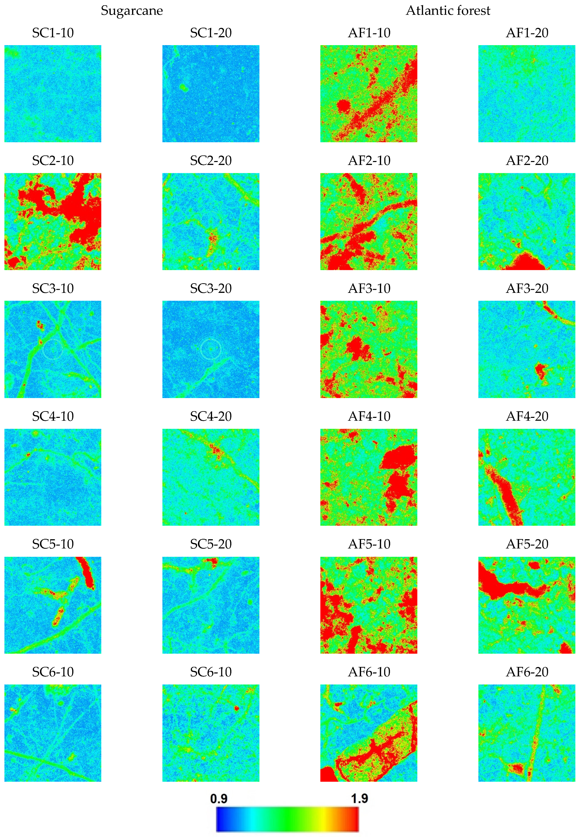
| Min | Q1 | Q2 | Q3 | Max | Mean | Stdev | |
|---|---|---|---|---|---|---|---|
| Atlantic Forest | |||||||
| AF1-10 | 1.05 | 1.36 | 1.51 | 1.72 | 4.30 | 1.58 | 3.22 × 10⁻¹ |
| AF2-10 | 1.02 | 1.36 | 1.53 | 1.79 | 4.61 | 1.63 | 3.89 × 10⁻¹ |
| AF3-10 | 1.03 | 1.33 | 1.46 | 1.65 | 4.13 | 1.54 | 3.11 × 10⁻¹ |
| AF4-10 | 1.03 | 1.30 | 1.44 | 1.68 | 5.08 | 1.58 | 4.53 × 10⁻¹ |
| AF5-10 | 1.02 | 1.35 | 1.54 | 1.84 | 4.69 | 1.65 | 4.22 × 10⁻¹ |
| AF6-10 | 1.01 | 1.14 | 1.32 | 1.64 | 5.48 | 1.47 | 4.74 × 10⁻¹ |
| AF1-20 | 1.01 | 1.12 | 1.17 | 1.24 | 2.29 | 1.19 | 1.00 × 10⁻¹ |
| AF2-20 | 1.01 | 1.14 | 1.21 | 1.33 | 4.13 | 1.29 | 2.69 × 10⁻¹ |
| AF3-20 | 1.01 | 1.11 | 1.16 | 1.23 | 4.13 | 1.20 | 1.61 × 10⁻¹ |
| AF4-20 | 1.01 | 1.18 | 1.27 | 1.40 | 3.58 | 1.34 | 2.55 × 10⁻¹ |
| AF5-20 | 1.01 | 1.22 | 1.34 | 1.55 | 4.85 | 1.47 | 4.17 × 10⁻¹ |
| AF6-20 | 1.01 | 1.13 | 1.21 | 1.31 | 2.71 | 1.25 | 1.68 × 10⁻¹ |
| Sugarcane | |||||||
| SC1-10 | 1.01 | 1.09 | 1.12 | 1.17 | 2.00 | 1.14 | 7.35 × 10⁻² |
| SC2-10 | 1.01 | 1.29 | 1.50 | 1.91 | 4.44 | 1.68 | 5.32 × 10⁻¹ |
| SC3-10 | 1.01 | 1.08 | 1.12 | 1.20 | 3.55 | 1.16 | 1.19 × 10⁻¹ |
| SC4-10 | 1.01 | 1.08 | 1.11 | 1.17 | 2.38 | 1.14 | 9.14 × 10⁻² |
| SC5-10 | 1.01 | 1.08 | 1.12 | 1.21 | 3.79 | 1.19 | 2.29 × 10⁻¹ |
| SC6-10 | 1.00 | 1.07 | 1.11 | 1.17 | 2.87 | 1.14 | 1.02 × 10⁻¹ |
| SC1-20 | 1.00 | 1.05 | 1.07 | 1.10 | 1.97 | 1.08 | 5.51 × 10⁻² |
| SC2-20 | 1.01 | 1.10 | 1.16 | 1.25 | 4.03 | 1.20 | 1.43 × 10⁻¹ |
| SC3-20 | 1.01 | 1.05 | 1.08 | 1.12 | 4.82 | 1.10 | 6.40 × 10⁻² |
| SC4-20 | 1.01 | 1.14 | 1.20 | 1.28 | 3.19 | 1.23 | 1.34 × 10⁻¹ |
| SC5-20 | 1.01 | 1.08 | 1.12 | 1.19 | 3.36 | 1.15 | 1.27 × 10⁻¹ |
| SC6-20 | 1.00 | 1.11 | 1.18 | 1.27 | 2.73 | 1.20 | 1.28 × 10⁻¹ |
References
- Labrière, N.; Locatelli, B.; Laumonier, Y.; Freycon, V.; Bernoux, M. Soil erosion in the humid tropics: A systematic quantitative review. Agric. Ecosyst. Environ. 2015, 203, 127–139. [Google Scholar] [CrossRef]
- Wohl, E.; Barros, A.; Brunsell, N.; Chappell, N.A.; Coe, M.; Giambelluca, T.; Goldsmith, S.; Harmon, R.; Hendrickx, J.M.H.; Juvik, J.; et al. The hydrology of the humid tropics. Nat. Clim. Chang. 2012, 2, 655–662. [Google Scholar] [CrossRef]
- Wilcke, W.; Yasin, S.; Abramowski, U.; Valarezo, C.; Zech, W. Nutrient storage and turnover in organic layers under tropical montane rain forest in Ecuador. Eur. J. Soil Sci. 2002, 53, 15–27. [Google Scholar] [CrossRef]
- Breuer, L.; Papen, H.; Butterbach-Bahl, K. N2O emission from tropical forest soils of Australia. J. Geophys. Res. Atmos. 2000, 105, 26353–26367. [Google Scholar] [CrossRef]
- Telles, E.d.C.C.; de Camargo, P.B.; Martinelli, L.A.; Trumbore, S.E.; da Costa, E.S.; Santos, J.; Higuchi, N.; Oliveira, R.C. Influence of soil texture on carbon dynamics and storage potential in tropical forest soils of Amazonia. Glob. Biogeochem. Cycles 2003, 17, 1040. [Google Scholar] [CrossRef]
- Fujii, K.; Shibata, M.; Kitajima, K.; Ichie, T.; Kitayama, K.; Turner, B.L. Plant–soil interactions maintain biodiversity and functions of tropical forest ecosystems. Ecol. Res. 2018, 33, 149–160. [Google Scholar] [CrossRef]
- Islam, K.R.; Weil, R.R. Land use effects on soil quality in a tropical forest ecosystem of Bangladesh. Agric. Ecosyst. Environ. 2000, 79, 9–16. [Google Scholar] [CrossRef]
- Lemenih, M.; Karltun, E.; Olsson, M. Assessing soil chemical and physical property responses to deforestation and subsequent cultivation in smallholders farming system in Ethiopia. Agric. Ecosyst. Environ. 2005, 105, 373–386. [Google Scholar] [CrossRef]
- Maharjan, M.; Sanaullah, M.; Razavi, B.S.; Kuzyakov, Y. Effect of land use and management practices on microbial biomass and enzyme activities in subtropical top-and sub-soils. Appl. Soil Ecol. 2017, 113, 22–28. [Google Scholar] [CrossRef]
- Zhou, H.; Peng, X.; Peth, S.; Xiao, T.Q. Effects of vegetation restoration on soil aggregate microstructure quantified with synchrotron-based micro-computed tomography. Soil Tillage Res. 2012, 124, 17–23. [Google Scholar] [CrossRef]
- Wang, M.; Xu, S.; Kong, C.; Zhao, Y.; Shi, X.; Guo, N. Assessing the effects of land use change from rice to vegetable on soil structural quality using X-ray CT. Soil Tillage Res. 2019, 195, 104343. [Google Scholar] [CrossRef]
- Rabot, E.; Wiesmeier, M.; Schlüter, S.; Vogel, H.-J. Soil structure as an indicator of soil functions: A review. Geoderma 2018, 314, 122–137. [Google Scholar] [CrossRef]
- Helliwell, J.R.; Sturrock, C.J.; Grayling, K.M.; Tracy, S.R.; Flavel, R.J.; Young, I.M.; Whalley, W.R. Applications of X-ray computed tomography for examining biophysical interactions and structural development in soil systems: A review. Eur. J. Soil Sci. 2013, 64, 279–297. [Google Scholar] [CrossRef]
- Schlüter, S.; Großmann, C.; Diel, J.; Wu, G.-M.; Tischer, S.; Deubel, A.; Jan Rücknagel, S.T.A.D. Long-term effects of conventional and reduced tillage on soil structure, soil ecological and soil hydraulic properties. Geoderma 2018, 332, 10–19. [Google Scholar] [CrossRef]
- Pires, L.F.; Roque, W.L.; Rosa, J.A.; Mooney, S.J. 3D analysis of the soil porous architecture under long term contrasting management systems by X-ray computed tomography. Soil Tillage Res. 2019, 191, 197–206. [Google Scholar] [CrossRef]
- Juarez, S.; Nunan, N.; Duday, A.-C.; Pouteau, V.; Schmidt, S.; Hapca, S.; Falconer, R.; Otten, W.; Chenu, C. Effects of different soil structures on the decomposition of native and added organic carbon. Eur. J. Soil Biol. 2013, 58, 81–90. [Google Scholar] [CrossRef]
- Galdos, M.V.; Pires, L.F.; Cooper, H.V.; Calonego, J.C.; Rosolem, C.A.; Mooney, S.J. Assessing the long-term effects of zero-tillage on the macroporosity of Brazilian soils using X-ray Computed Tomography. Geoderma 2019, 337, 1126–1135. [Google Scholar] [CrossRef]
- Santos, C.R.D.; Antonino, A.C.D.; Heck, R.J.; Lucena, L.R.R.d.; Oliveira, A.C.H.d.; Silva, A.S.A.d.; Stosic, B.; Menezes, R.S.C. 3D soil void space lacunarity as an index of degradation after land use change. Acta Scientiarum. Agron. 2020, 42, e42491. [Google Scholar] [CrossRef]
- Perret, J.S.; Prasher, S.O.; Kacimov, A.R. Mass fractal dimension of soil macropores using computed tomography: From the box-counting to the cube-counting algorithm. Eur. J. Soil Sci. 2003, 54, 569–579. [Google Scholar] [CrossRef]
- Wang, J.; Guo, L.; Bai, Z.; Yang, L. Using computed tomography (CT) images and multi-fractal theory to quantify the pore distribution of reconstructed soils during ecological restoration in opencast coal-mine. Ecol. Eng. 2016, 92, 148–157. [Google Scholar] [CrossRef]
- Martínez, F.S.J.; Martín, M.; Caniego, F.; Tuller, M.; Guber, A.; Pachepsky, Y.; García-Gutiérrez, C. Multifractal analysis of discretized X-ray CT images for the characterization of soil macropore structures. Geoderma 2010, 156, 32–42. [Google Scholar] [CrossRef]
- Torre, I.G.; Martín-Sotoca, J.J.; Losada, J.C.; López, P.; Tarquis, A.M. Scaling properties of binary and greyscale images in the context of X-ray soil tomography. Geoderma 2020, 365, 114205. [Google Scholar] [CrossRef]
- Mooney, S.J.; Korošak, D. Using complex networks to model two-and three-dimensional soil porous architecture. Soil Sci. Soc. Am. J. 2009, 73, 1094–1100. [Google Scholar] [CrossRef]
- Samec, M.; Santiago, A.; Cárdenas, J.P.; Benito, R.M.; Tarquis, A.M.; Mooney, S.J.; Korošak, D. Quantifying soil complexity using network models of soil porous structure. Nonlinear Process. Geophys. 2013, 20, 41–45. [Google Scholar] [CrossRef]
- Tarquis, A.M.; Heck, R.J.; Andina, D.; Alvarez, A.; Antón, J.M. Pore network complexity and thresholding of 3D soil images. Ecol. Complex. 2009, 6, 230–239. [Google Scholar] [CrossRef]
- Zhou, H.; Perfect, E.; Li, B.G.; Lu, Y.Z. Effects of bit depth on the multifractal analysis of grayscale images. Fractals 2010, 18, 127–138. [Google Scholar] [CrossRef]
- Zhou, H.; Perfect, E.; Lu, Y.Z.; Li, B.G.; Peng, X.H. Multifractal analyses of grayscale and binary soil thin section images. Fractals 2011, 19, 299–309. [Google Scholar] [CrossRef]
- Roy, A.; Perfect, E. Lacunarity analyses of multifractal and natural grayscale patterns. Fractals 2014, 22, 1440003. [Google Scholar] [CrossRef]
- Torre, I.G.; Losada, J.C.; Heck, R.J.; Tarquis, A.M. Multifractal analysis of 3D images of tillage soil. Geoderma 2018, 311, 167–174. [Google Scholar] [CrossRef]
- Torre, I.G.; Losada, J.C.; Tarquis, A.M. Multiscaling properties of soil images. Biosyst. Eng. 2018, 168, 133–141. [Google Scholar] [CrossRef]
- IBGE. Contas de Ecossistemas: O uso da Terra nos Biomas Brasileiros: 2000–2018; IBGE: Rio de Janeiro, Brazil, 2020.
- CONAB. Acompanhamento da Safra Brasileira de Cana-de-Açúcar; CONAB: Brasilia, Brazil, 2020.
- Ortiz, P.F.S.; Rolim, M.M.; de Lima, J.L.P.; Pedrosa, E.M.R.; Dantas, M.S.M.; Tavares, U.E. Physical qualities of an Ultisol under sugarcane and Atlantic forest in Brazil. Geoderma Reg. 2017, 11, 62–70. [Google Scholar] [CrossRef]
- de Oliveira Bordonal, R.; Carvalho, J.L.N.; Lal, R.; de Figueiredo, E.B.; de Oliveira, B.G.; La Scala, N. Sustainability of sugarcane production in Brazil. A review. Agron. Sustain. Dev. 2018, 38, 1–23. [Google Scholar]
- Castioni, G.A.; Cherubin, M.R.; Menandro, L.M.S.; Sanches, G.M.; Bordonal, R.d.O.; Barbosa, L.C.; Franco, H.C.J.; Carvalho, J.L.N. Soil physical quality response to sugarcane straw removal in Brazil: A multi-approach assessment. Soil Tillage Res. 2018, 184, 301–309. [Google Scholar] [CrossRef]
- Cavalcanti, R.Q.; Rolim, M.M.; de Lima, R.P.; Tavares, U.E.; Pedrosa, E.M.R.; Cherubin, M.R. Soil physical changes induced by sugarcane cultivation in the Atlantic Forest biome, northeastern Brazil. Geoderma 2020, 370, 114353. [Google Scholar] [CrossRef]
- Vignat, C.; Bercher, J.-F. Analysis of signals in the Fisher–Shannon information plane. Phys. Lett. A 2003, 312, 27–33. [Google Scholar] [CrossRef]
- Martin, M.T.; Pennini, F.; Plastino, A. Fisher’s information and the analysis of complex signals. Phys. Lett. A 1999, 256, 173–180. [Google Scholar] [CrossRef]
- Fisher, R.A. Theory of statistical estimation. Math. Proc. Camb. Philos. Soc. 1925, 22, 700–725. [Google Scholar] [CrossRef]
- Estañón, C.R.; Aquino, N.; Puertas-Centeno, D.; Dehesa, J.S. Two-dimensional confined hydrogen: An entropy and complexity approach. Int. J. Quantum Chem. 2020, 120, e26192. [Google Scholar] [CrossRef]
- Frieden, B.R. Fisher information, disorder, and the equilibrium distributions of physics. Phys. Rev. A 1990, 41, 4265. [Google Scholar] [CrossRef]
- Moreno-Torres, L.R.; Gomez-Vieyra, A.; Lovallo, M.; Ram’irez-Rojas, A.; Telesca, L. Investigating the interaction between rough surfaces by using the Fisher–Shannon method: Implications on interaction between tectonic plates. Phys. A Stat. Mech. Its Appl. 2018, 506, 560–565. [Google Scholar] [CrossRef]
- Suleimanov, B.A.; Guseinova, N.I. Analyzing the state of oil field development based on the Fisher and Shannon information measures. Autom. Remote Control 2019, 80, 882–896. [Google Scholar] [CrossRef]
- Ba, R.; Song, W.; Lovallo, M.; Lo, S.; Telesca, L. Analysis of multifractal and organization/order structure in Suomi-NPP VIIRS normalized difference vegetation index series of wildfire affected and unaffected sites by using the multifractal detrended fluctuation analysis and the Fisher–Shannon analysis. Entropy 2020, 22, 415. [Google Scholar] [CrossRef] [PubMed]
- Lovallo, M.; Telesca, L. Complexity measures and information planes of X-ray astrophysical sources. J. Stat.Mech. Theory Exp. 2011, 2011, P03029. [Google Scholar] [CrossRef]
- Pierini, J.O.; Lovallo, M.; Gómez, E.A.; Telesca, L. Fisher–Shannon analysis of the time variability of remotely sensed sea surface temperature at the Brazil–Malvinas Confluence. Oceanologia 2016, 58, 187–195. [Google Scholar] [CrossRef]
- Stosic, T.; Telesca, L.; Stosic, B. Multiparametric statistical and dynamical analysis of angular high-frequency wind speed time series. Phys. A Stat. Mech. Its Appl. 2021, 566, 125627. [Google Scholar] [CrossRef]
- da Silva, A.S.A.; Menezes, R.S.C.; Telesca, L.; Stosic, B.; Stosic, T. Fisher Shannon analysis of drought/wetness episodes along a rainfall gradient in Northeast Brazil. Int. J. Climatol. 2021, 41, E2097–E2110. [Google Scholar] [CrossRef]
- Li, X.; Telesca, L.; Lovallo, M.; Xu, X.; Zhang, J.; Song, W. Spectral and informational analysis of pedestrian contact force in simulated overcrowding conditions. Phys. A Stat. Mech. Its Appl. 2020, 555, 124614. [Google Scholar] [CrossRef]
- Angulo, J.C.; Antolin, J.; Sen, K.D. Fisher–Shannon plane and statistical complexity of atoms. Phys. Lett. A 2008, 372, 670–674. [Google Scholar] [CrossRef]
- Dembo, A.; Cover, T.M.; Thomas, J.A. Information theoretic inequalities. IEEE Trans. Inf. Theory 1991, 37, 1501–1518. [Google Scholar] [CrossRef]
- Telesca, L.; Lovallo, M. On the performance of Fisher Information Measure and Shannon entropy estimators. Phys. A Stat. Mech. Its Appl. 2017, 484, 569–576. [Google Scholar] [CrossRef]
- Raykar, V.C.; Duraiswami, R. Fast optimal bandwidth selection for kernel density estimation. In Proceedings of the 2006 SIAM International Conference on Data Mining, Bethesda, MD, USA, 20–22 April 2006; pp. 524–528. [Google Scholar]
- Silverman, B.W. Density Estimation for Statistics and Data Analysis; Chapman & Hall: London, UK, 1986. [Google Scholar] [CrossRef]


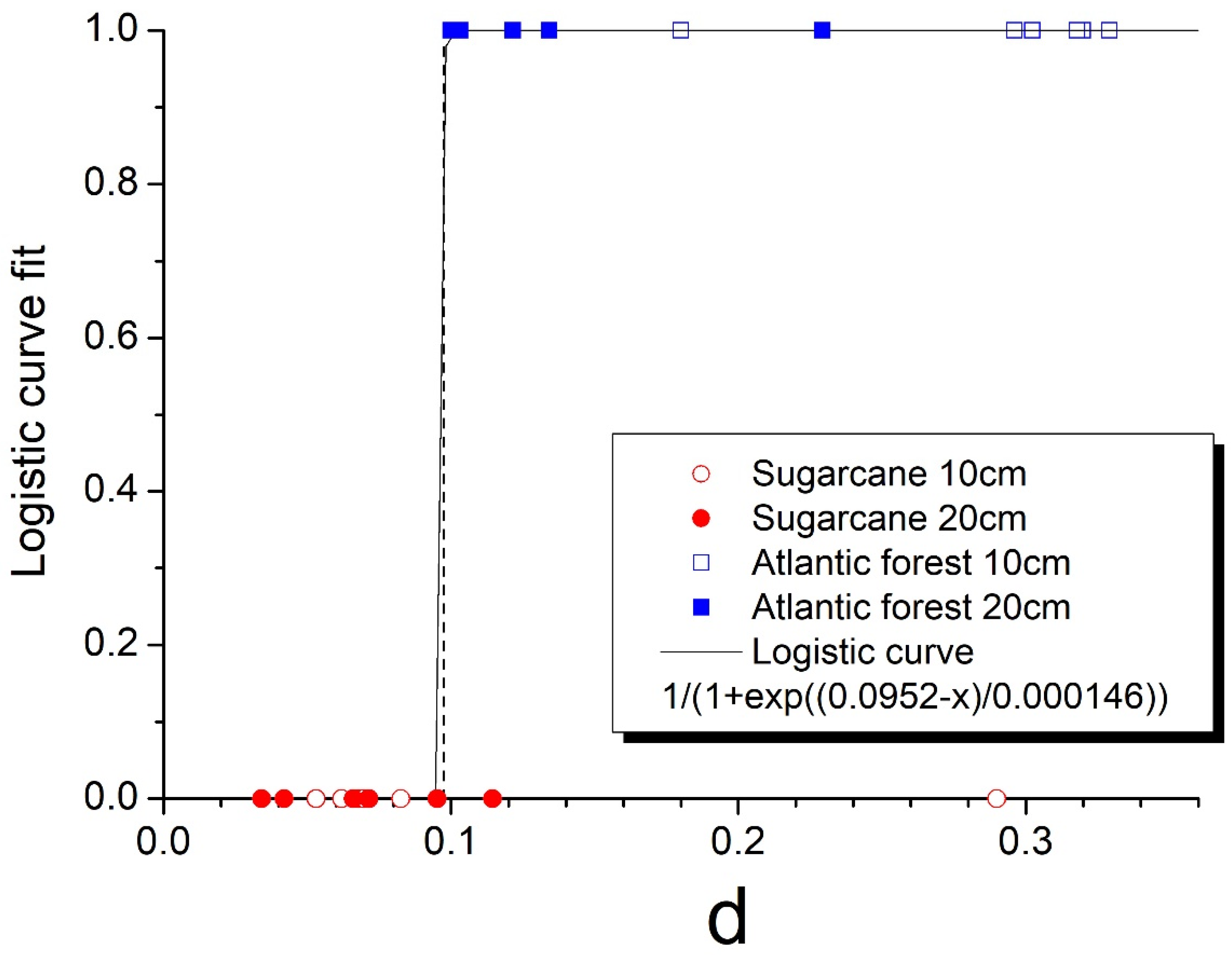
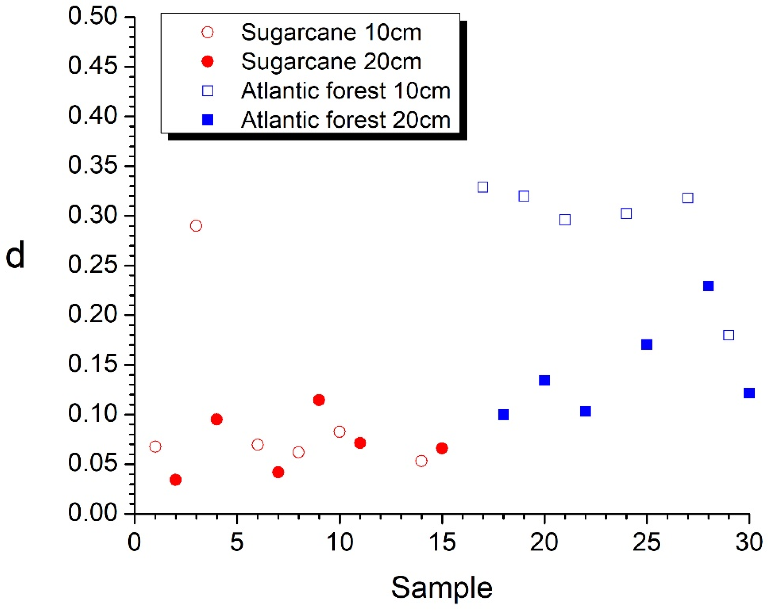
| Sugarcane | |||||
|---|---|---|---|---|---|
| SC1-10 | SC2-10 | SC3-10 | SC4-10 | SC5-10 | SC6-10 |
| 0.0676 | 0.2899 | 0.0696 | 0.0619 | 0.0825 | 0.0531 |
| SC1-20 | SC2-20 | SC3-20 | SC4-20 | SC5-20 | SC6-20 |
| 0.0342 | 0.0951 | 0.0420 | 0.1144 | 0.0714 | 0.0660 |
| Atlantic forest | |||||
| AF1-10 | AF2-10 | AF3-10 | AF4-10 | AF5-10 | AF6-10 |
| 0.3290 | 0.3198 | 0.2961 | 0.3022 | 0.3179 | 0.1799 |
| AF1-20 | AF2-20 | AF3-20 | AF4-20 | AF5-20 | AF6-20 |
| 0.0998 | 0.1341 | 0.1032 | 0.1704 | 0.2294 | 0.1215 |
Disclaimer/Publisher’s Note: The statements, opinions and data contained in all publications are solely those of the individual author(s) and contributor(s) and not of MDPI and/or the editor(s). MDPI and/or the editor(s) disclaim responsibility for any injury to people or property resulting from any ideas, methods, instructions or products referred to in the content. |
© 2023 by the authors. Licensee MDPI, Basel, Switzerland. This article is an open access article distributed under the terms and conditions of the Creative Commons Attribution (CC BY) license (https://creativecommons.org/licenses/by/4.0/).
Share and Cite
Aguiar, D.; Menezes, R.S.C.; Antonino, A.C.D.; Stosic, T.; Tarquis, A.M.; Stosic, B. Quantifying Soil Complexity Using Fisher Shannon Method on 3D X-ray Computed Tomography Scans. Entropy 2023, 25, 1465. https://doi.org/10.3390/e25101465
Aguiar D, Menezes RSC, Antonino ACD, Stosic T, Tarquis AM, Stosic B. Quantifying Soil Complexity Using Fisher Shannon Method on 3D X-ray Computed Tomography Scans. Entropy. 2023; 25(10):1465. https://doi.org/10.3390/e25101465
Chicago/Turabian StyleAguiar, Domingos, Rômulo Simões Cezar Menezes, Antonio Celso Dantas Antonino, Tatijana Stosic, Ana M. Tarquis, and Borko Stosic. 2023. "Quantifying Soil Complexity Using Fisher Shannon Method on 3D X-ray Computed Tomography Scans" Entropy 25, no. 10: 1465. https://doi.org/10.3390/e25101465
APA StyleAguiar, D., Menezes, R. S. C., Antonino, A. C. D., Stosic, T., Tarquis, A. M., & Stosic, B. (2023). Quantifying Soil Complexity Using Fisher Shannon Method on 3D X-ray Computed Tomography Scans. Entropy, 25(10), 1465. https://doi.org/10.3390/e25101465