


Tsallis Entropy and Mutability to Characterize Seismic Sequences: The Case of 2007–2014 Northern Chile Earthquakes

 ,
, 
 and
and
Abstract
:1. Introduction
2. Methodology
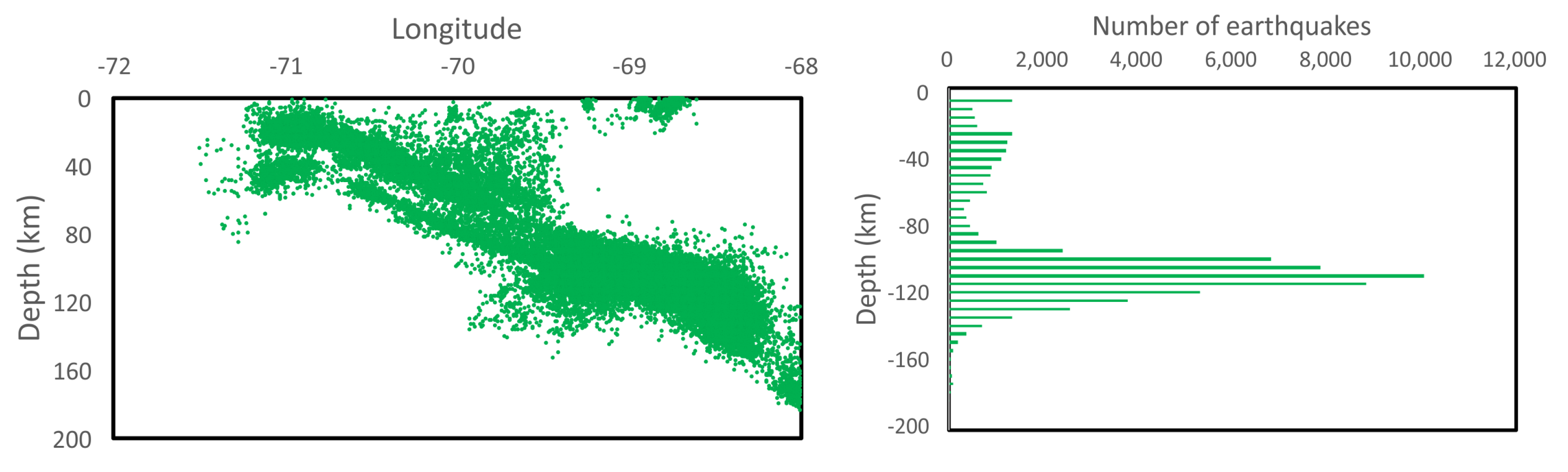
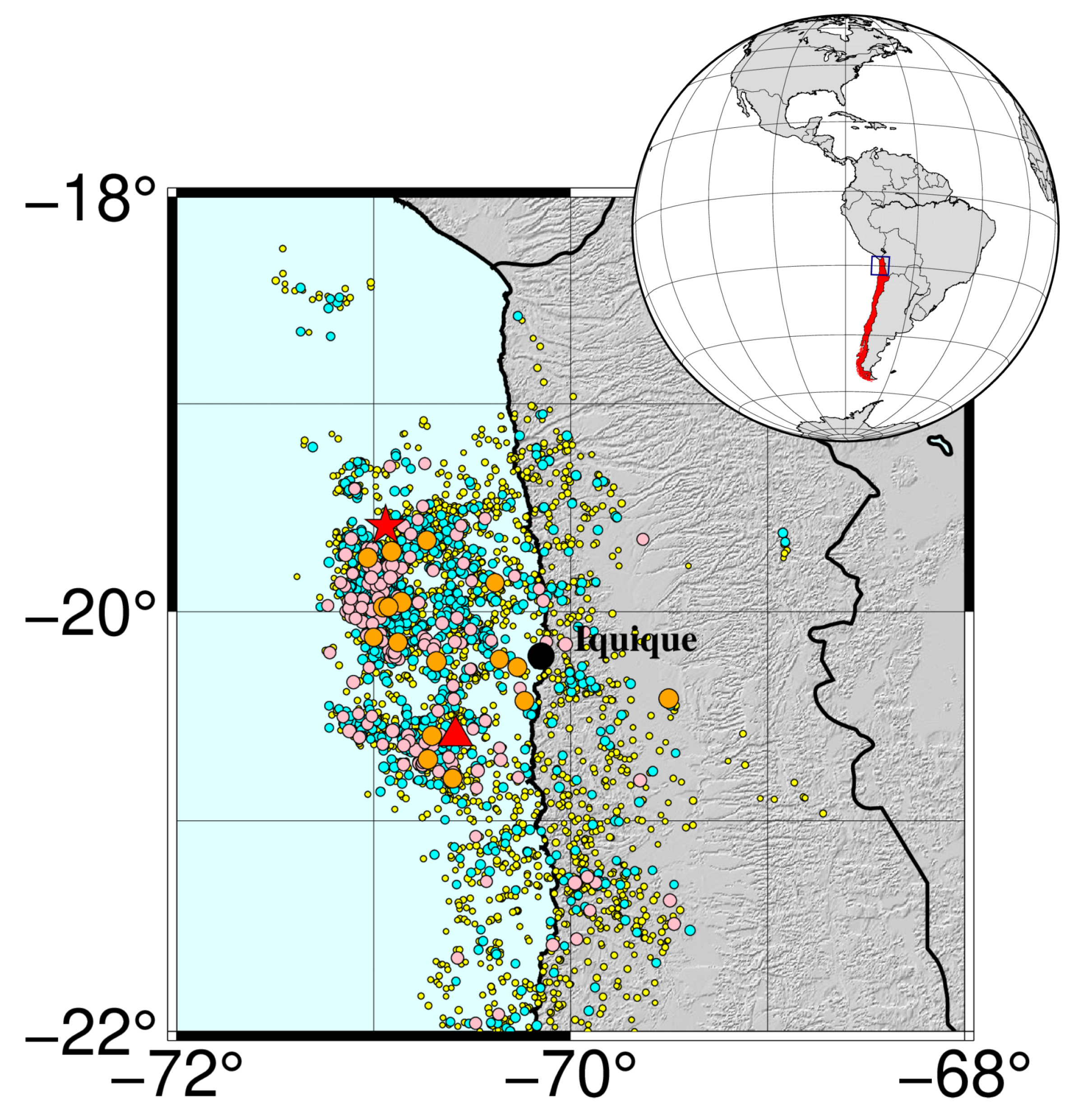
2.1. Data Source
2.2. Handling of Data
2.3. Tsallis Entropy
2.4. Mutability
2.5. Algorithm of the Data Recognizer
- (a)
- Navigate to the first register of the original file, copy it onto the compressed file as a first register followed by a space and then the digit 0 to indicate the beginning or origin of the new file.
- (b)
- Select the following register in the original file and compare it to the already stored register(s) in the compressed file.
- -
- If this register already exists then navigate to its row, leave a space and write to the right the “distance” or number of registers since it was previously found in the original file.
- -
- If the register repeats itself immediately after, place a comma and the number of consecutive repetitions.
- -
- If this register is new, then write it at a new row followed a space and then the distance to the first register.
- (c)
- Navigate to next register and repeat the procedure given in (b) until the last register in the file.
2.6. Tuning the Information Recognizer
- (i)
- Is this a static calculation (entire file, just once) or a dynamical calculation through time windows? Answer: it is dynamic through windows with W registers.
- (ii)
- Are these successive independent or overlapping windows? Answer: we use overlapping successive windows.
- (iii)
- If they overlap, what is the size of the overlap? We consider here a displacement of just one register between consecutive windows so the overlap is events.
- (iv)
- In step (b) of the algorithm described above, a numeric comparison is performed between two registers. How many digits and which digits bear the most sensitive information to perform this comparison? An estimation is possible after inspecting the data, but we let wlzip itself find the digits that lead to a better precision. The comparison is restricted to the r digits from position i and the following digits; this is denoted (i,r). In the examples of Table 1, all comparisons were for i = 1, r = 3 (the dot needs to be compared as well).
- (v)
- If precision is needed, wlzip has the feature of handling different numeric bases (quaternary, binary, ...) which can help to discriminate intermediate positions.
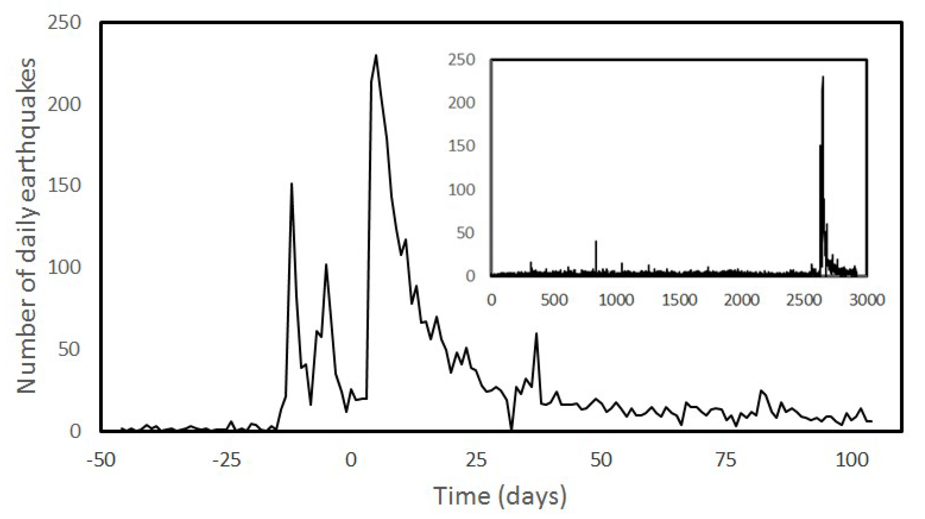
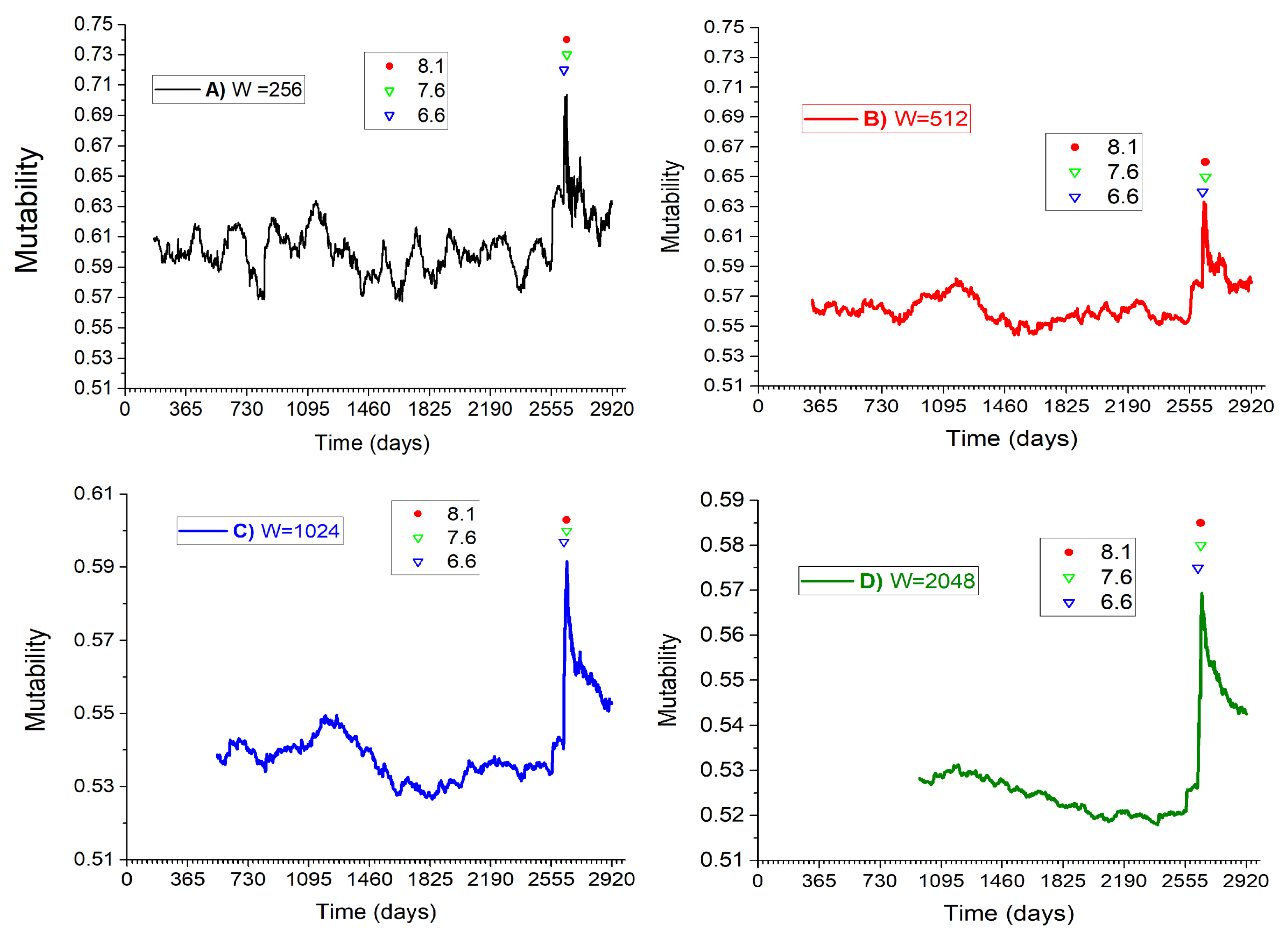
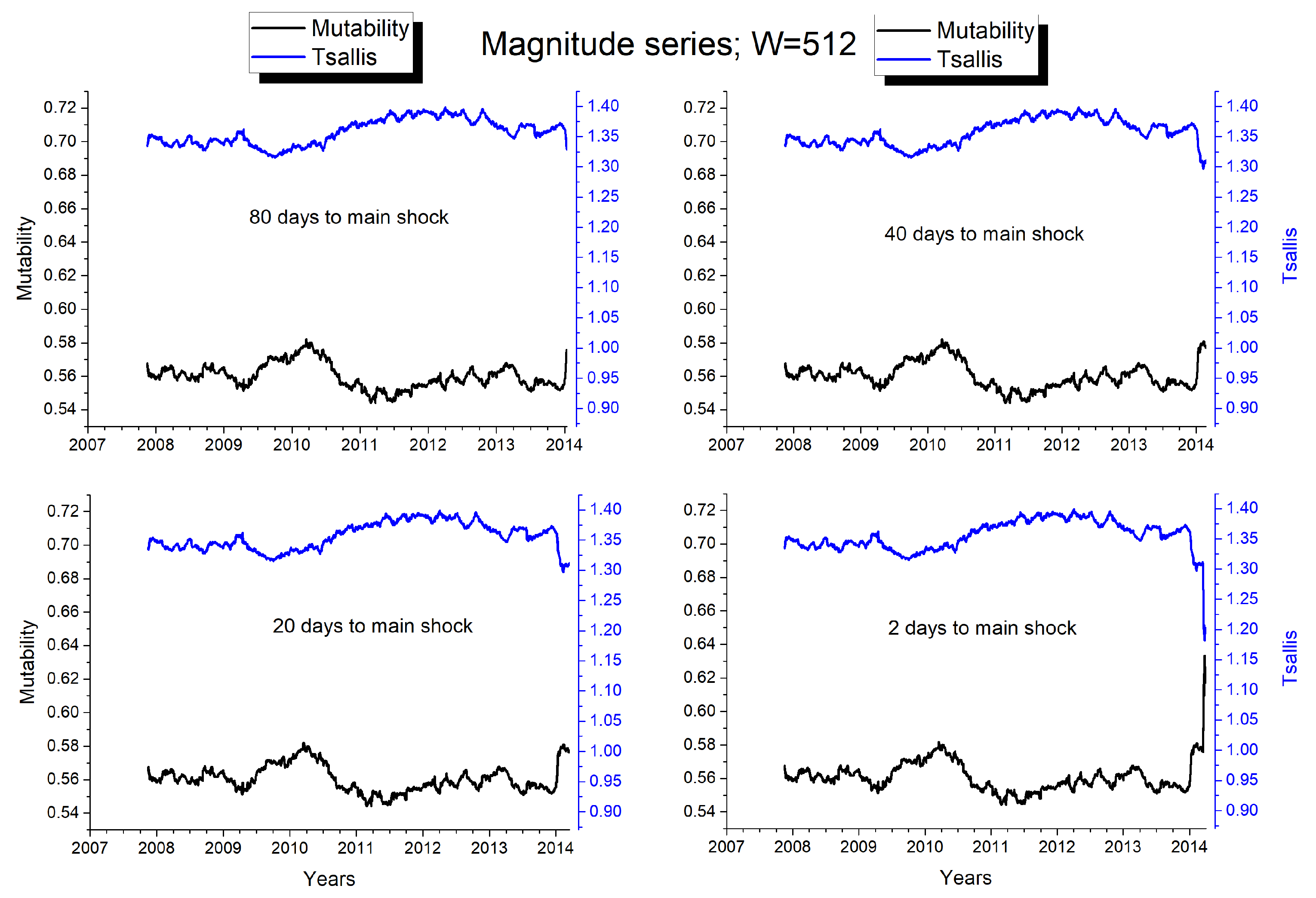
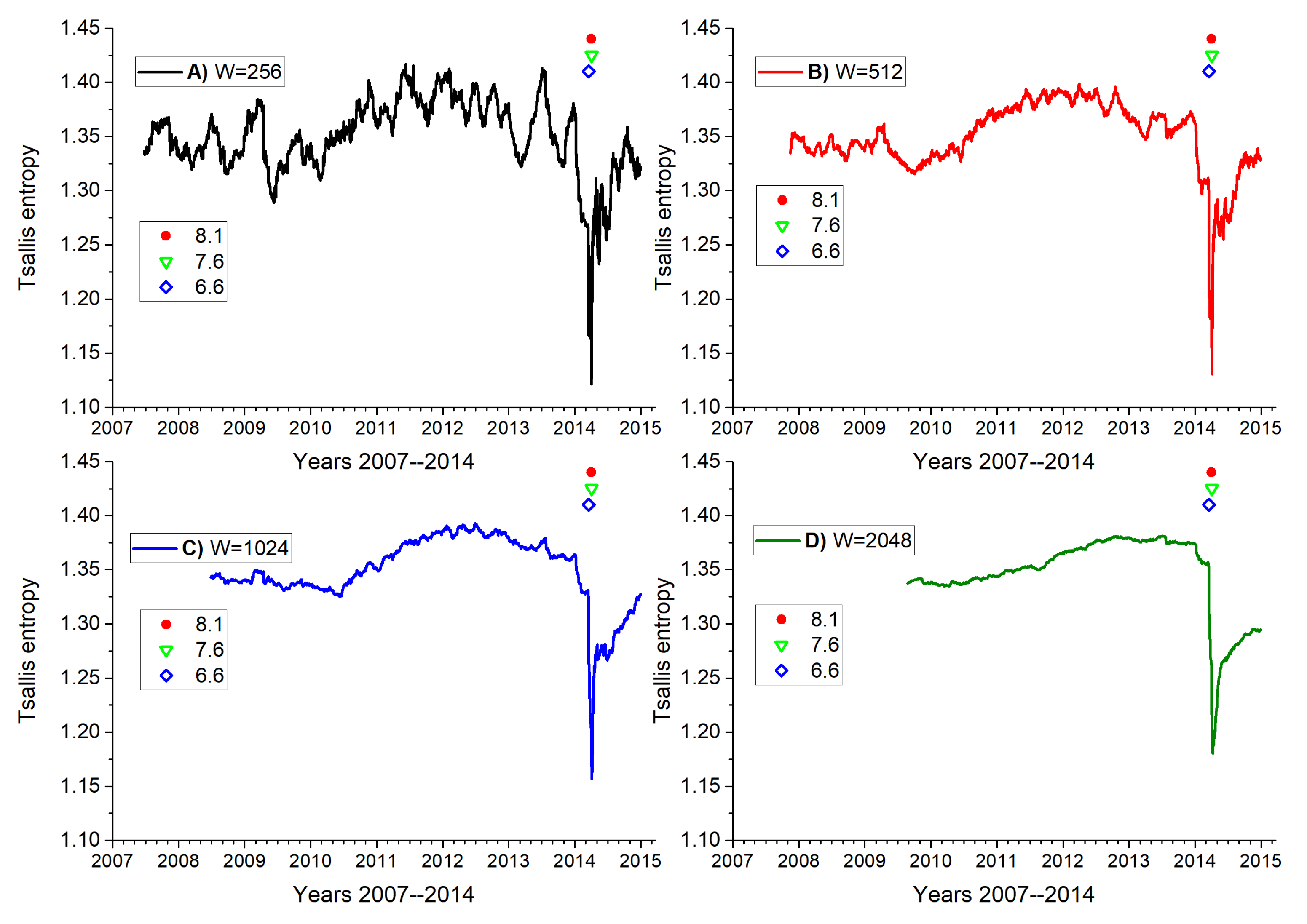
3. Results
4. Conclusions
Author Contributions
Funding
Data Availability Statement
Conflicts of Interest
References
- Zhang, Y.; Zuo, T.; Cheng, Y.; Liaw, P. High-entropy Alloys with High Saturation Magnetization, Electrical Resistivity and Malleability. Sci. Rep. 2013, 3, 1455. [Google Scholar] [CrossRef] [PubMed]
- Oumezzine, M.; Peña, O.; Kallel, S.; Zemni, S. Critical phenomena and estimation of the spontaneous magnetization through magnetic entropy change in La0.67Ba0.33Mn0.98Ti0.02O3. Solid State Sci. 2011, 13, 1829–1834. [Google Scholar] [CrossRef]
- Sauerwein, R.A.; de Oliveira, M.J. Entropy of spin models by the Monte Carlo method. Phys. Rev. B 1995, 52, 3060–3062. [Google Scholar] [CrossRef]
- Zhang, Y.; Grover, T.; Vishwanath, A. Entanglement Entropy of Critical Spin Liquids. Phys. Rev. Lett. 2011, 107, 067202. [Google Scholar] [CrossRef] [PubMed]
- Wand, A.J.; Sharp, K.A. Measuring Entropy in Molecular Recognition by Proteins. Annu. Rev. Biophys. 2018, 47, 41–61. [Google Scholar] [CrossRef]
- Nezhad, S.Y.; Deiters, U.K. Estimation of the entropy of fluids with Monte Carlo computer simulation. Mol. Phys. 2017, 115, 1074–1085. [Google Scholar] [CrossRef]
- Johnson, J.R.; Wing, S.; Camporeale, E. Transfer entropy and cumulant-based cost as measures of nonlinear causal relationships in space plasmas: Applications to Dst. Ann. Geophys. 2018, 36, 945–952. [Google Scholar] [CrossRef]
- Du, S.; Zank, G.P.; Li, X.; Guo, F. Energy dissipation and entropy in collisionless plasma. Phys. Rev. E 2020, 101, 033208. [Google Scholar] [CrossRef]
- Bailey, K. Social Entropy Theory: An overview. Syst. Pract. 1990, 3, 365–382. [Google Scholar] [CrossRef]
- Liu, Z.; Wang, Y.; Cheng, Q.; Yang, H. Analysis of the Information Entropy on Traffic Flows. IEEE Trans. Intell. Transp. Syst. 2022, 23, 18012–18023. [Google Scholar] [CrossRef]
- Liu, F.J.; Chang, T.P. Validity analysis of maximum entropy distribution based on different moment constraints for wind energy assessment. Energy 2011, 36, 1820–1826. [Google Scholar] [CrossRef]
- Sarlis, N.; Skordas, E.; Varotsos, P. Nonextensivity and natural time: The case of seismicity. Phys. Rev. E 2010, 82, 021110. [Google Scholar] [CrossRef]
- Telesca, L. Maximum likelihood estimation of the nonextensive parameters of the earthquake cumulative magnitude distribution. Bull. Seismol. Soc. Am. 2012, 102, 886–891. [Google Scholar] [CrossRef]
- Varotsos, P.; Sarlis, N.; Skordas, E. Tsallis Entropy Index q and the Complexity Measure of Seismicity in Natural Time under Time Reversal before the M9 Tohoku Earthquake in 2011. Entropy 2018, 20, 757. [Google Scholar] [CrossRef] [PubMed]
- Posadas, A.; Morales, J.; Ibáñez, J.; Posadas, A. Shaking earth: Non-linear seismic processes and the second law of thermodynamics: A case study from Canterbury (New Zealand) earthquakes. Chaos Solitons Fractals Nonlinear Sci. Nonequilibrium Complex Phenom. 2022, 151, 111243. [Google Scholar] [CrossRef]
- Skordas, E.; Sarlis, N.; Varotsos, P. Precursory variations of Tsallis non-extensive statistical mechanics entropic index associated with the M9 Tohoku earthquake in 2011. Eur. Phys. J. Spec. Top. 2020, 229, 851–859. [Google Scholar] [CrossRef]
- Sigalotti, L.; Ramírez-Rojas, A.; Vargas, C. Tsallis q-Statistics in Seismology. Entropy 2023, 25, 408. [Google Scholar] [CrossRef]
- Santis, A.D.; Cianchini, G.; Favali, P.; Beranzoli, L.; Boschi, E. The Gutenberg-Richter Law and Entropy of Earthquakes: Two Case Studies in Central Italy. Bull. Seismol. Soc. Am. 2011, 101, 1386–1395. [Google Scholar] [CrossRef]
- Vogel, E.E.; Brevis, F.G.; Pastén, D.; Muñoz, V.; Miranda, R.A.; Chian, A.C.-L. Measuring the sismic risk along the Nazca-South American subduction front: Shannon entropy and mutability. Nat. Hazards Earth Syst. Sci. 2020, 20, 2943–2960. [Google Scholar] [CrossRef]
- Sotolongo-Costa, O.; Posadas, A. Fragment-asperity interaction model for earthquakes. Phys. Rev. Lett. 2004, 92, 048501. [Google Scholar] [CrossRef]
- Posadas, A.; Sotolongo-Costa, O. Non-extensive entropy and fragment–asperity interaction model for earthquakes. Commun. Nonlinear Sci. Numer. Simul. 2023, 117, 106906. [Google Scholar] [CrossRef]
- Varotsos, P.A.; Sarlis, N.; Skordas, E.S.; Uyeda, S.; Kamogawa, M. Natural time analysis of critical phenomena. Proc. Natl. Acad. Sci. USA 2011, 108, 11361–11364. [Google Scholar] [CrossRef]
- Varotsos, P.A.; Sarlis, N.V.; Skordas, E.S. Phenomena preceding major earthquakes interconnected through a physical model. Ann. Geophys. 2019, 37, 315–324. [Google Scholar] [CrossRef]
- Posadas, A.; Pasten, D.; Vogel, E.E.; Saravia, G. Earthquake hazard characterization by using entropy: Application to northern Chilean earthquakes. Nat. Hazards Earth Syst. Sci. 2023, 23, 1911–1920. [Google Scholar] [CrossRef]
- Béjar-Pizarro, M.; Socquet, A.; Armijo, R.; Carrizo, D.; Genrich, J.; Simons, M. Andean structural control on interseismic coupling in the North Chile subduction zone. Nat. Geosci. 2013, 6, 462–467. [Google Scholar] [CrossRef]
- Comte, D.; Pardo, M. Reappraisal of great historical earthquakes in the Northern Chile and Southern Peru seismic gaps. Nat. Hazards 1991, 4, 23–44. [Google Scholar] [CrossRef]
- Métois, M.; Vigny, C.; Socquet, A. Interseismic Coupling, Megathrust Earthquakes and Seismic Swarms Along the Chilean Subduction Zone 38 °S–18 °S. Pure Appl. Geophys. 2016, 173, 1431–1449. [Google Scholar] [CrossRef]
- Delouis, B.; Monfret, T.; Dorbath, L.; Pardo, M.; Rivera, L.; Comte, D.; Haessler, H.; Caminade, J.; Ponce, L.; Kausel, E.; et al. The Mw 8.0 Antofagasta (northern Chile) earthquake of 30 July 1995: A precursor to the end of the large 1877 gap. Bull. Seismol. Soc. Am. 1997, 87, 427–445. [Google Scholar] [CrossRef]
- Peyrat, S.; Campos, J.; de Chabalier, J.B.; Bonvalot, S.; Bouin, M.P.; Legrand, D.; Nercessian, A.; Charade, O.; Patau, G.; Clévédé, E.; et al. Tarapacá intermediate-depth earthquake (Mw 7.7, 2005, northern Chile): A slab-pull event with horizontal fault plane constrained from seismologic and geodetic observations. Geophys. Res. Lett. 2006, 33, L22308. [Google Scholar] [CrossRef]
- Schurr, B.; Asch, G.; Rosenau, M.; Wang, R.; Oncken, O.; Barrientos, S.; Salazar, P.; Vilotte, J.P. The 2007 Mw7.7 Tocopilla northern Chile earthquake sequence: Implications for along-strike and downdip rupture segmentationand megathrust frictional behavior. J. Geophys. Res. 2012, 117, 1–19. [Google Scholar]
- Leon-Rios, S.; Ruiz, S.; Maksymowicz, A.; Leyton, F.; Fuenzalida, A.; Madariaga, R. Diversity of the 2014 Iquique’s foreshocks and aftershocks: Clues about the complex rupture process of a Mw8.1 earthquake. J. Seismol. 2016, 20, 1059–1073. [Google Scholar] [CrossRef]
- Ruiz, S.; Métois, M.; Fuenzalida, A.; Ruiz, J.; Leyton, F.; Grandin, R.; Vigny, C.; Madariaga, R.; Campos, J. Intense foreshocks and a slow slip event preceded the 2014 Iquique Mw 8.1 earthquake. Science 2014, 345, 1165–1169. [Google Scholar] [CrossRef] [PubMed]
- Ruiz, S.; Madariaga, R. Historical and recent large megathrust earthquakes in Chile. Tectonophysics 2018, 733, 37–56. [Google Scholar] [CrossRef]
- Socquet, A.; Valdes, J.P.; Jara, J.; Cotton, F.; Walpersdorf, A.; Cotte, N.; Specht, S.; Ortega-Culaciati, F.; Carrizo, D.; Norabuena, E. An 8 month slow slip event triggers progressive nucleation of the 2014 Chile megathrust. Geophys. Res. Lett. 2017, 44, 4046–4053. [Google Scholar] [CrossRef]
- Jara, J.; Socquet, A.; Marsan, D.; Bouchon, M. Long-Term Interactions Between Intermediate Depth and Shallow Seismicity in North Chile Subduction Zone. Geophys. Res. Lett. 2017, 44, 9283–9292. [Google Scholar] [CrossRef]
- IPOC. Available online: https://www.ipoc-network.org/welcome-to-ipoc/ (accessed on 25 August 2023).
- Brodsky, E.E.; Lay, T. Recognizing foreshocks from the 1 April 2014 Chile earthquake. Science 2014, 344, 700–702. [Google Scholar] [CrossRef]
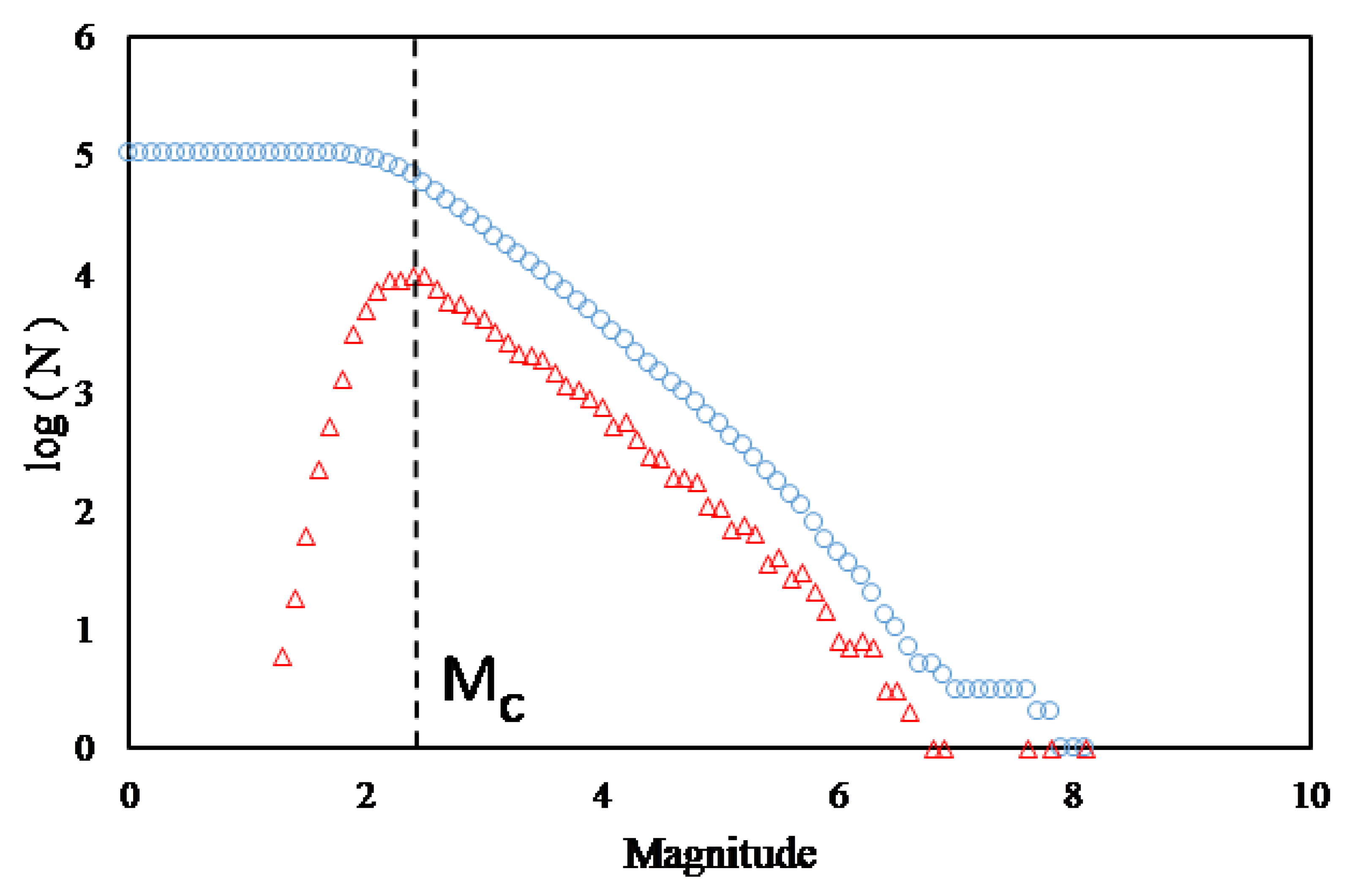
- Wiemer, S.; Wyss, M. Minimum magnitude of complete reporting in earthquake catalogs: Examples from Alaska, the Western United States, and Japan. Bull. Seismol. Soc. Am. 2000, 90, 859–869. [Google Scholar] [CrossRef]
- Telesca, L. Tsallis-based nonextensive analysis of the southern California seismicity. Entropy 2011, 13, 1267–1280. [Google Scholar] [CrossRef]
- Papadakis, G.; Vallianatos, F.; Sammonds, P. A nonextensive statistical physics analysis of the 1995 Kobe, Japan earthquake. Pure Appl. Geophys. 2015, 172, 1923–1931. [Google Scholar] [CrossRef]
- Varotsos, P.; Sarlis, N.; Skordas, E. Identifying the occurrence time of an impending major earthquake: A review. Earthq. Sci. 2017, 30, 209–218. [Google Scholar] [CrossRef]
- Santis, A.D.; Abbattista, C.; Alfonsi, L.; Amoruso, L.; Campuzano, S.; Carbone, M.; Cesaroni, C.; Cianchini, G.; Franceschi, G.D.; Santis, A.D.; et al. Geosystemics View of Earthquakes. Entropy 2019, 21, 412. [Google Scholar] [CrossRef]
- Vallianatos, F.; Michas, G.; Papadakis, G. A description of seismicity based on non-extensive statistical physics: A review. In Earthquakes and Their Impact on Society; D’Amico, S., Ed.; Springer Natural Hazards: Cham, Switzerland, 2015; pp. 1–41. [Google Scholar]
- Vilar, C.; Franca, G.; Silva, R.; Alcaniz, J. Nonextensivity in geological faults? Phys. A 2007, 377, 285–290. [Google Scholar] [CrossRef]
- Michas, G. Generalized Statistical Mechanics Description of Fault and Earthquake Populations in Corinth Rift (Greece). PhD. Thesis, University College London, London, UK, 2016. [Google Scholar]
- Telesca, L. Analysis of Italian seismicity by using a nonextensive approach. Tectonophysics 2010, 494, 155–162. [Google Scholar] [CrossRef]
- Khordad, R.; Rastegar Sedehi, H.; Sharifzadeh, M. Susceptibility, entropy and specific heat of quantum rings in monolayer graphene: Comparison between different entropy formalisms. J. Comput. Electron. 2022, 21, 422–430. [Google Scholar] [CrossRef]
- Aki, K. Maximum likelihood estimate of b in the formula log (N) = a – bm and its confidence limits. Bull. Earthq. Res. Inst. Tokyo Univ. 1965, 43, 237–239. [Google Scholar]
- Utsu, T. A method for determining the value of b in a formula log n = a – bm showing the magnitude-frequency relation for earthquakes. Geophys. Bull. Hokkaido 1965, 13, 99–103. [Google Scholar]
- Luenberg, D.G. Information Science, 2nd ed.; Princeton University Press: Princeton, NJ, USA, 2006. [Google Scholar]
- Cover, T.M.; Thomas, J.A. Elements of Information Theory, 2nd ed.; John Wiley and Sons: New York, NY, USA, 2006. [Google Scholar]
- Roederer, J.G. Information and Its Role in Nature, 2nd ed.; Springer: Heidelberg, Germany, 2005. [Google Scholar]
- Vogel, E.; Saravia, G.; Bachmann, F.; Fierro, B.; Fischer, J. Phase transitions in Edwards-Anderson model by means of information theory. Phys. A 2009, 388, 4075–4082. [Google Scholar] [CrossRef]
- Vogel, E.; Saravia, G.; Cortez, L. Data compressor designed to improve recognition of magnetic phases. Phys. A 2012, 391, 1591–1601. [Google Scholar] [CrossRef]
- Negrete, O.A.; Vargas, P.; Peña, F.J.; Saravia, G.; Vogel, E.E. Entropy and mutability for the q-State Clock Model in Small Systems. Renew. Energy 2018, 20, 933. [Google Scholar] [CrossRef]
- Vogel, E.; Saravia, G. Information Theory Applied to Econophysics: Stock Market Behaviors. Eur. J. Phys. B 2014, 87, 177. [Google Scholar] [CrossRef]
- Vogel, E.; Saravia, G.; Ramirez-Pastor, A. Phase transitions in a system of long rods on two-dimensional lattices by means of information theory. Phys. Rev. E 2017, 96, 062133. [Google Scholar] [CrossRef] [PubMed]
- Dos Santos, G.; Cisternas, E.; Vogel, E.E.; Ramirez-Pastor, A.J. Orientational phase transition in monolayers of multipolar straight ridid rods: The case of 2-thiophene molecule adsorption on the Au (111) surface. Phys. Rev. E 2023, 107, 014133. [Google Scholar] [CrossRef] [PubMed]
- Vogel, E.E.; Saravia, G.; Kobe, S.; Schumann, R.; Schuster, R. A Novel Method to Optimize Electricity Generation from Wind Energy. Renew. Energy 2018, 126, 724–735. [Google Scholar] [CrossRef]
- Universidad de Chile (2013): Red Sismologica Nacional. International Federation of Digital Seismograph Networks. Other/Seismic Network. 10.7914/SN/C1. Available online: https://www.fdsn.org/networks/detail/C1/ (accessed on 12 April 2022).
- Vogel, E.; Saravia, G.; Pastén, D.; Muñoz, V. Time-series analysis of earthquake sequences by means of information recognizer. Tectonophysics 2017, 712–713, 723–728. [Google Scholar] [CrossRef]


| Before | After | |||||
|---|---|---|---|---|---|---|
| n | M | MapB | M | MapA | ||
| 1 | 2.4 | 0 18 10 7 4 | 5 | 6.6 | 0 | 1 |
| 2 | 4.0 | 1 2 44,2 | 4 | 4.5 | 1 | 1 |
| 3 | 3.8 | 2 34 | 2 | 4.8 | 2 4 5 10 | 4 |
| 4 | 2.2 | 4 4 14 11,2 8 | 6 | 4.1 | 3 26 | 2 |
| 5 | 4.6 | 5 | 1 | 3.1 | 4 6 3 3 22,2 9 | 7 |
| 6 | 3.5 | 6 11 2 | 3 | 5.2 | 5 | 1 |
| 7 | 2.9 | 7 22 20 | 3 | 4.2 | 7 | 1 |
| 8 | 3.0 | 9 | 1 | 3.8 | 8 28 | 2 |
| 9 | 4.1 | 10 27 | 2 | 3.5 | 9 10 4 | 3 |
| 10 | 3.1 | 11,2 | 2 | 3.7 | 12 32 4 | 3 |
| 11 | 4.3 | 13,2 | 2 | 3.6 | 14 | 1 |
| 12 | 3.6 | 15 | 1 | 3.3 | 15 18 10 | 3 |
| 13 | 5.5 | 16 | 1 | 4.0 | 17 14 | 2 |
| 14 | 2.7 | 20 | 1 | 2.7 | 18 | 1 |
| 15 | 2.5 | 21 2 2 15 2 3 | 6 | 3.2 | 20 8 | 2 |
| 16 | 2.3 | 24 8 12 | 3 | 2.8 | 22 | 1 |
| 17 | 2.6 | 26 4 | 2 | 2.4 | 24 | 1 |
| 18 | 3.3 | 27 | 1 | 4.7 | 25 12 4 4 | 4 |
| 19 | 2.8 | 31 7 5 | 3 | 3.0 | 26 20 | 2 |
| 20 | 3.4 | 46 | 1 | 2.9 | 27 | 1 |
| 21 | 4.3 | 30 4 | 2 | |||
| 22 | 5.1 | 32 | 1 | |||
| 23 | 3.4 | 35 7 7 | 3 | |||
| 24 | 2.6 | 40 | 1 | |||
Disclaimer/Publisher’s Note: The statements, opinions and data contained in all publications are solely those of the individual author(s) and contributor(s) and not of MDPI and/or the editor(s). MDPI and/or the editor(s) disclaim responsibility for any injury to people or property resulting from any ideas, methods, instructions or products referred to in the content. |
© 2023 by the authors. Licensee MDPI, Basel, Switzerland. This article is an open access article distributed under the terms and conditions of the Creative Commons Attribution (CC BY) license (https://creativecommons.org/licenses/by/4.0/).
Share and Cite
Pasten, D.; Vogel, E.E.; Saravia, G.; Posadas, A.; Sotolongo, O. Tsallis Entropy and Mutability to Characterize Seismic Sequences: The Case of 2007–2014 Northern Chile Earthquakes. Entropy 2023, 25, 1417. https://doi.org/10.3390/e25101417
Pasten D, Vogel EE, Saravia G, Posadas A, Sotolongo O. Tsallis Entropy and Mutability to Characterize Seismic Sequences: The Case of 2007–2014 Northern Chile Earthquakes. Entropy. 2023; 25(10):1417. https://doi.org/10.3390/e25101417
Chicago/Turabian StylePasten, Denisse, Eugenio E. Vogel, Gonzalo Saravia, Antonio Posadas, and Oscar Sotolongo. 2023. "Tsallis Entropy and Mutability to Characterize Seismic Sequences: The Case of 2007–2014 Northern Chile Earthquakes" Entropy 25, no. 10: 1417. https://doi.org/10.3390/e25101417
APA StylePasten, D., Vogel, E. E., Saravia, G., Posadas, A., & Sotolongo, O. (2023). Tsallis Entropy and Mutability to Characterize Seismic Sequences: The Case of 2007–2014 Northern Chile Earthquakes. Entropy, 25(10), 1417. https://doi.org/10.3390/e25101417