

Multifidelity Model Calibration in Structural Dynamics Using Stochastic Variational Inference on Manifolds


Abstract
:1. Introduction
2. Multifidelity Gaussian Process Modeling and Calibration
2.1. Autoregressive Gaussian Processes
2.2. Posterior Distribution
3. Variational Inference
Black-Box Variational Inference
4. Stochastic Optimization
Manifold Gradient Ascent
| Algorithm 1: Manifold gradient ascent |
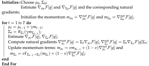 |
5. Numerical Examples
5.1. Academic Example
5.2. Chicago Crimes Statistics Dataset
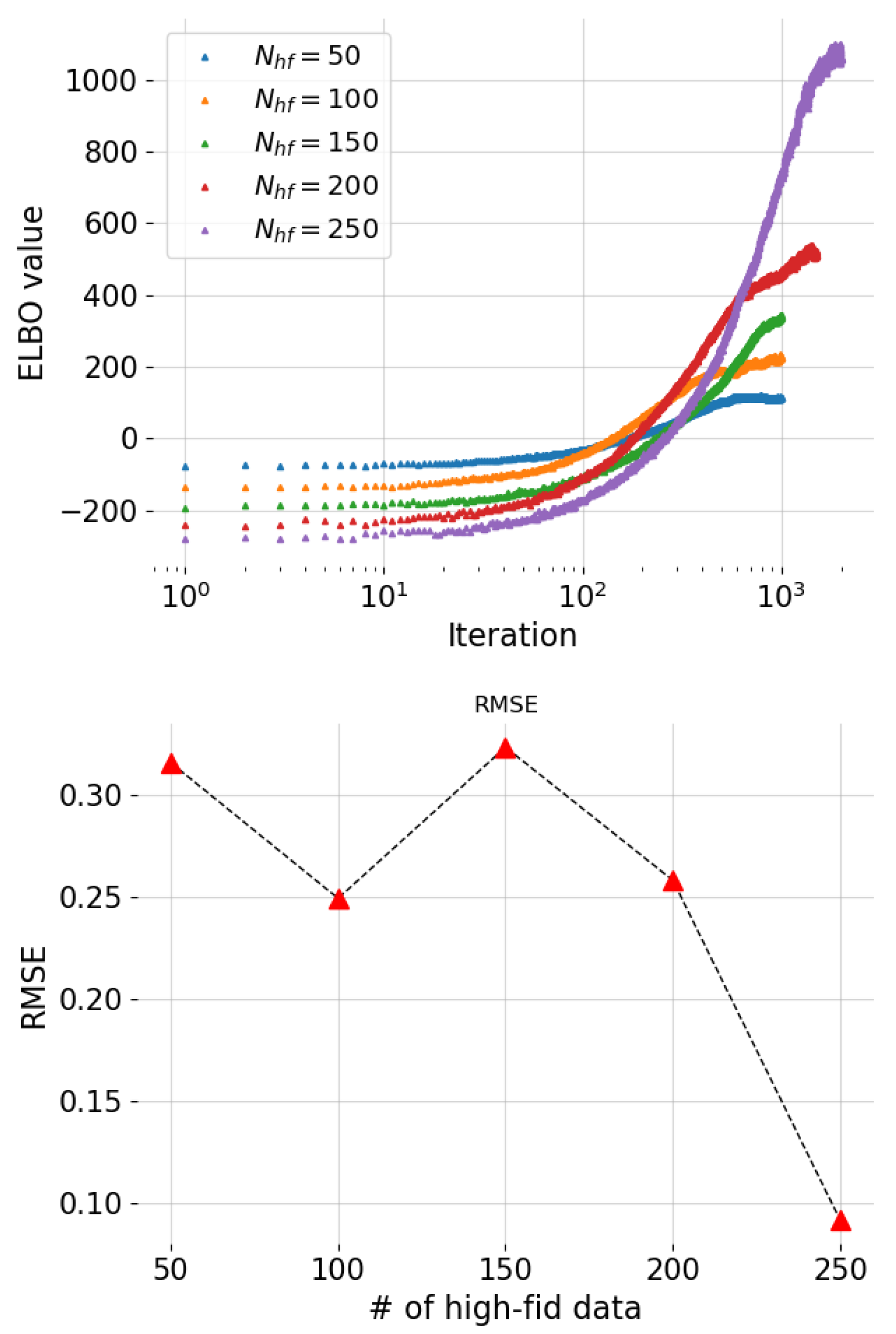
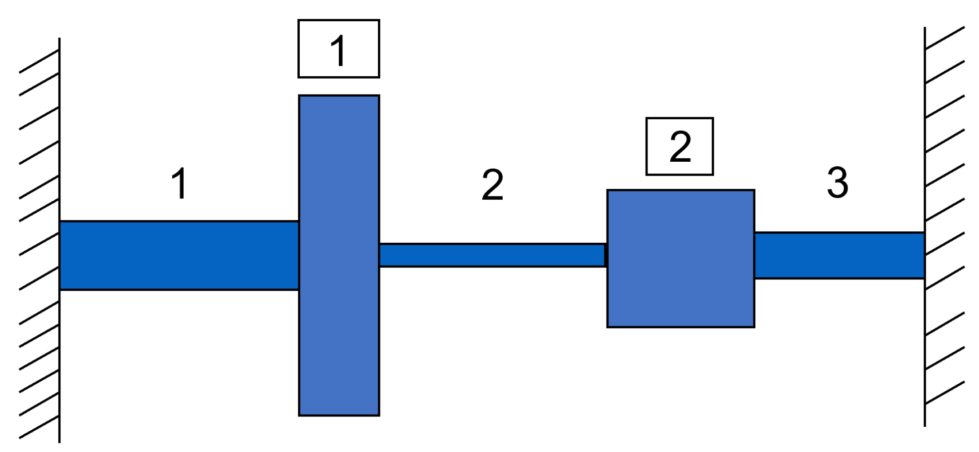
5.3. Torsional Vibration Problem
6. Conclusions
Author Contributions
Funding
Institutional Review Board Statement
Informed Consent Statement
Data Availability Statement
Conflicts of Interest
References
- Hill, W.J.; Hunter, W.G. A review of response surface methodology: A literature survey. Technometrics 1966, 8, 571–590. [Google Scholar] [CrossRef]
- Vaidya, S.; Ambad, P.; Bhosle, S. Industry 4.0—A glimpse. Procedia Manuf. 2018, 20, 233–238. [Google Scholar] [CrossRef]
- Rasmussen, C.E. Gaussian Processes in Machine Learning; Summer School on Machine Learning; Springer: Berlin/Heidelberg, Germany, 2003; pp. 63–71. [Google Scholar]
- Hensman, J.; Fusi, N.; Lawrence, N.D. Gaussian processes for Big data. In Proceedings of the Twenty-Ninth Conference on Uncertainty in Artificial Intelligence, Bellevue, WA, USA, 11–15 August 2013; pp. 282–290. [Google Scholar]
- Damianou, A.; Lawrence, N.D. Deep gaussian processes. In Proceedings of the Sixteenth International Conference on Artificial Intelligence and Statistics, Scottsdale, AZ, USA, 29 August 2013; pp. 207–215. [Google Scholar]
- Goodfellow, I.; Bengio, Y.; Courville, A. Deep Learning; MIT Press: Cambridge, MA, USA, 2016. [Google Scholar]
- Gal, Y.; Ghahramani, Z. Dropout as a bayesian approximation: Representing model uncertainty in deep learning. In Proceedings of the International Conference on Machine Learning, New York, NY, USA, 19–24 June 2016; pp. 1050–1059. [Google Scholar]
- Lakshminarayanan, B.; Pritzel, A.; Blundell, C. Simple and Scalable Predictive Uncertainty Estimation using Deep Ensembles. Adv. Neural Inf. Process. Syst. 2017, 30, 1–12. [Google Scholar]
- Ghanem, R.; Spanos, P.D. Polynomial chaos in stochastic finite elements. J. Appl. Mech. 1990, 57, 197–202. [Google Scholar] [CrossRef]
- Tsilifis, P.; Ghanem, R.G. Reduced Wiener chaos representation of random fields via basis adaptation and projection. J. Comput. Phys. 2017, 341, 102–120. [Google Scholar] [CrossRef]
- Sa, G.; Liu, Z.; Qiu, C.; Peng, X.; Tan, J. Novel Performance-Oriented Tolerance Design Method Based on Locally Inferred Sensitivity Analysis and Improved Polynomial Chaos Expansion. J. Mech. Des. 2021, 143, 022001. [Google Scholar] [CrossRef]
- Pandita, P.; Bilionis, I.; Panchal, J.; Gautham, B.; Joshi, A.; Zagade, P. Stochastic multiobjective optimization on a budget: Application to multipass wire drawing with quantified uncertainties. Int. J. Uncertain. Quantif. 2018, 8, 233–249. [Google Scholar] [CrossRef]
- Pandita, P.; Bilionis, I.; Panchal, J. Bayesian optimal design of experiments for inferring the statistical expectation of expensive black-box functions. J. Mech. Des. 2019, 141, 101404. [Google Scholar] [CrossRef]
- Pandita, P.; Bilionis, I.; Panchal, J. Extending expected improvement for high-dimensional stochastic optimization of expensive black-box functions. J. Mech. Des. 2016, 138, 111412. [Google Scholar] [CrossRef]
- Tsilifis, P.; Huan, X.; Safta, C.; Sargsyan, K.; Lacaze, G.; Oefelein, J.C.; Najm, H.N.; Ghanem, R.G. Compressive sensing adaptation for polynomial chaos expansions. J. Comput. Phys. 2019, 380, 29–47. [Google Scholar] [CrossRef]
- Hu, Z.; Hu, C.; Mourelatos, Z.P.; Mahadevan, S. Model discrepancy quantification in simulation-based design of dynamical systems. J. Mech. Des. 2019, 141, 011401. [Google Scholar] [CrossRef]
- Peherstorfer, B.; Willcox, K.; Gunzburger, M. Survey of multifidelity methods in uncertainty propagation, inference, and optimization. Siam Rev. 2018, 60, 550–591. [Google Scholar] [CrossRef]
- Nobile, F.; Tesei, F. A Multi Level Monte Carlo method with control variate for elliptic PDEs with log-normal coefficients. Stoch. Partial Differ. Equ. Anal. Comput. 2015, 3, 398–444. [Google Scholar] [CrossRef]
- Benner, P.; Gugercin, S.; Willcox, K. A survey of projection-based model reduction methods for parametric dynamical systems. SIAM Rev. 2015, 57, 483–531. [Google Scholar] [CrossRef]
- Forrester, A.; Keane, A. Recent advances in surrogate-based optimization. Prog. Aerosp. Sci. 2009, 45, 50–79. [Google Scholar] [CrossRef]
- Forrester, A.; Sóbester, A.; Keane, A. Multi-fidelity optimization via surrogate modelling. Proc. R. Soc. A Math. Phys. Eng. Sci. 2007, 463, 3251–3269. [Google Scholar] [CrossRef]
- Huan, X.; Safta, C.; Sargsyan, K.; Vane, Z.; Lacaze, G.; Oefelein, J.; Najm, H. Compressive sensing with cross-validation and stop-sampling for sparse polynomial chaos expansions. SIAM/ASA J. Uncertain. Quantif. 2018, 6, 907–936. [Google Scholar] [CrossRef]
- Tsilifis, P.; Pandita, P.; Ghosh, S.; Andreoli, V.; Vandeputte, T.; Wang, L. Bayesian learning of orthogonal embeddings for multi-fidelity Gaussian Processes. Comput. Methods Appl. Mech. Eng. 2021, 386, 114147. [Google Scholar] [CrossRef]
- Liu, H.; Ong, Y.S.; Shen, X.; Cai, J. When Gaussian process meets big data: A review of scalable GPs. IEEE Trans. Neural Netw. Learn. Syst. 2020, 31, 4405–4423. [Google Scholar] [CrossRef]
- Wang, K.; Pleiss, G.; Gardner, J.; Tyree, S.; Weinberger, K.Q.; Wilson, A.G. Exact Gaussian processes on a million data points. Adv. Neural Inf. Process. Syst. 2019, 32, 14648–14659. [Google Scholar]
- Berns, F.; Beecks, C. Towards Large-scale Gaussian Process Models for Efficient Bayesian Machine Learning. In Proceedings of the 9th International Conference on Data Science, Technology and Applications—DATA, Paris, France, 7–9 July 2020; pp. 275–282. [Google Scholar] [CrossRef]
- Tran, A.; Eldred, M.; McCann, S.; Wang, Y. srMO-BO-3GP: A sequential regularized multi-objective Bayesian optimization for constrained design applications using an uncertain Pareto classifier. J. Mech. Des. 2022, 144, 031705. [Google Scholar] [CrossRef]
- Ghosh, S.; Pandita, P.; Atkinson, S.; Subber, W.; Zhang, Y.; Kumar, N.C.; Chakrabarti, S.; Wang, L. Advances in bayesian probabilistic modeling for industrial applications. ASCE-ASME J. Risk Uncertain. Eng. Syst. Part B Mech. Eng. 2020, 6, 030904. [Google Scholar] [CrossRef]
- Pandita, P.; Tsilifis, P.; Ghosh, S.; Wang, L. Scalable Fully Bayesian Gaussian Process Modeling and Calibration with Adaptive Sequential Monte Carlo for Industrial Applications. J. Mech. Des. 2021, 143, 074502. [Google Scholar] [CrossRef]
- Cui, T.; Law, K.J.; Marzouk, Y.M. Dimension-independent likelihood-informed MCMC. J. Comput. Phys. 2016, 304, 109–137. [Google Scholar] [CrossRef]
- Parno, M.D.; Marzouk, Y.M. Transport map accelerated markov chain monte carlo. SIAM/ASA J. Uncertain. Quantif. 2018, 6, 645–682. [Google Scholar] [CrossRef]
- Peherstorfer, B.; Marzouk, Y. A transport-based multifidelity preconditioner for Markov chain Monte Carlo. Adv. Comput. Math. 2019, 45, 2321–2348. [Google Scholar] [CrossRef]
- El Moselhy, T.A.; Marzouk, Y.M. Bayesian inference with optimal maps. J. Comput. Phys. 2012, 231, 7815–7850. [Google Scholar] [CrossRef]
- Ranganath, R.; Gerrish, S.; Blei, D. Black box variational inference. In Proceedings of the Artificial Intelligence and Statistics, Reykjavic, Iceland, 22–25 April 2014; pp. 814–822. [Google Scholar]
- Blei, D.; Kucukelbir, A.; McAuliffe, J. Variational inference: A review for statisticians. J. Am. Stat. Assoc. 2017, 112, 859–877. [Google Scholar] [CrossRef]
- Titsias, M.; Lázaro-Gredilla, M. Doubly stochastic variational Bayes for non-conjugate inference. In Proceedings of the International Conference on Machine Learning, Beijing, China, 21–26 June 2014; pp. 1971–1979. [Google Scholar]
- Tsilifis, P.; Ghanem, R. Bayesian adaptation of chaos representations using variational inference and sampling on geodesics. Proc. R. Soc. A Math. Phys. Eng. Sci. 2018, 474, 20180285. [Google Scholar] [CrossRef]
- Tsilifis, P.; Papaioannou, I.; Straub, D.; Nobile, F. Sparse Polynomial Chaos expansions using variational relevance vector machines. J. Comput. Phys. 2020, 416, 109498. [Google Scholar] [CrossRef]
- Tsilifis, P.; Bilionis, I.; Katsounaros, I.; Zabaras, N. Computationally efficient variational approximations for Bayesian inverse problems. J. Verif. Valid. Uncertain. Quantif. 2016, 1, 031004. [Google Scholar] [CrossRef]
- Graves, A. Practical variational inference for neural networks. Adv. Neural Inf. Process. Syst. 2011, 24, 2348–2356. [Google Scholar]
- Paisley, J.; Blei, D.M.; Jordan, M.I. Variational Bayesian inference with stochastic search. In Proceedings of the 29th International Coference on International Conference on Machine Learning, Edinburgh, UK, 26 June–1 July 2012; pp. 1363–1370. [Google Scholar]
- Deshpande, S.; Purwar, A. Computational creativity via assisted variational synthesis of mechanisms using deep generative models. J. Mech. Des. 2019, 141, 121402. [Google Scholar] [CrossRef]
- Hoffman, M.; Blei, D.; Wang, C.; Paisley, J. Stochastic variational inference. J. Mach. Learn. Res. 2013, 14, 111401. [Google Scholar]
- Salimbeni, H.; Deisenroth, M. Doubly stochastic variational inference for deep Gaussian processes. arXiv 2017, arXiv:1705.08933. [Google Scholar]
- Hoang, T.; Hoang, Q.; Low, B. A unifying framework of anytime sparse Gaussian process regression models with stochastic variational inference for big data. In Proceedings of the International Conference on Machine Learning, Lille, France, 6–11 July 2015; pp. 569–578. [Google Scholar]
- Kennedy, M.; O’Hagan, A. Bayesian calibration of computer models. J. R. Stat. Soc. Ser. B Stat. Methodol. 2001, 63, 425–464. [Google Scholar] [CrossRef]
- Kennedy, M.; O’Hagan, A. Predicting the output from a complex computer code when fast approximations are available. Biometrika 2000, 87, 1–13. [Google Scholar] [CrossRef]
- Le Gratiet, L.; Garnier, J. Recursive co-kriging model for design of computer experiments with multiple levels of fidelity. Int. J. Uncertain. Quantif. 2014, 4, 365–386. [Google Scholar] [CrossRef]
- Le Gratiet, L. Bayesian analysis of hierarchical multifidelity codes. SIAM/ASA J. Uncertain. Quantif. 2013, 1, 244–269. [Google Scholar] [CrossRef]
- Arendt, P.D.; Apley, D.W.; Chen, W.; Lamb, D.; Gorsich, D. Improving identifiability in model calibration using multiple responses. J. Mech. Des. 2012, 134, 100909. [Google Scholar] [CrossRef]
- Arendt, P.D.; Apley, D.W.; Chen, W. A preposterior analysis to predict identifiability in the experimental calibration of computer models. IIE Trans. 2016, 48, 75–88. [Google Scholar] [CrossRef]
- Tuo, R.; Jeff Wu, C. A theoretical framework for calibration in computer models: Parametrization, estimation and convergence properties. SIAM/ASA J. Uncertain. Quantif. 2016, 4, 767–795. [Google Scholar] [CrossRef]
- Hoffman, M.; Bach, F.; Blei, D. Online learning for latent Dirichlet allocation. In Proceedings of the Advances in Neural Information Processing Systems, Vancouver, BC, Canada, 6–9 December 2010; pp. 856–864. [Google Scholar]
- Wainwright, M.; Jordan, M. Graphical models, exponential families, and variational inference. Found. Trends® Mach. Learn. 2008, 1, 1–305. [Google Scholar] [CrossRef]
- Wang, C.; Blei, D. Variational Inference in Nonconjugate Models. J. Mach. Learn. Res. 2013, 14, 1005–1031. [Google Scholar]
- Amari, S. Natural gradient works efficiently in learning. Neural Comput. 1998, 10, 251–276. [Google Scholar] [CrossRef]
- Martens, J. New insights and perspectives on the natural gradient method. J. Mach. Learn. Res. 2020, 21, 1–76. [Google Scholar]
- Absil, P.; Mahony, R.; Sepulchre, R. Optimization Algorithms on Matrix Manifolds; Princeton University Press: Princeton, NJ, USA, 2009. [Google Scholar]
- Roy, S.; Harandi, M. Constrained stochastic gradient descent: The good practice. In Proceedings of the 2017 International Conference on Digital Image Computing: Techniques and Applications (DICTA), Sydney, Australia, 29 November–1 December 2017; pp. 1–8. [Google Scholar]
- Savva, F.; Anagnostopoulos, C.; Triantafillou, P. Explaining aggregates for exploratory analytics. In Proceedings of the 2018 IEEE International Conference on Big Data (Big Data), Seattle, WA, USA, 10–13 December 2018; pp. 478–487. [Google Scholar]
- Anagnostopoulos, C.; Savva, F.; Triantafillou, P. Scalable aggregation predictive analytics. Appl. Intell. 2018, 48, 2546–2567. [Google Scholar] [CrossRef] [Green Version]
- GPy. GPy: A Gaussian Process Framework in Python. Since 2012. Available online: http://github.com/SheffieldML/GPy (accessed on 1 January 2022).


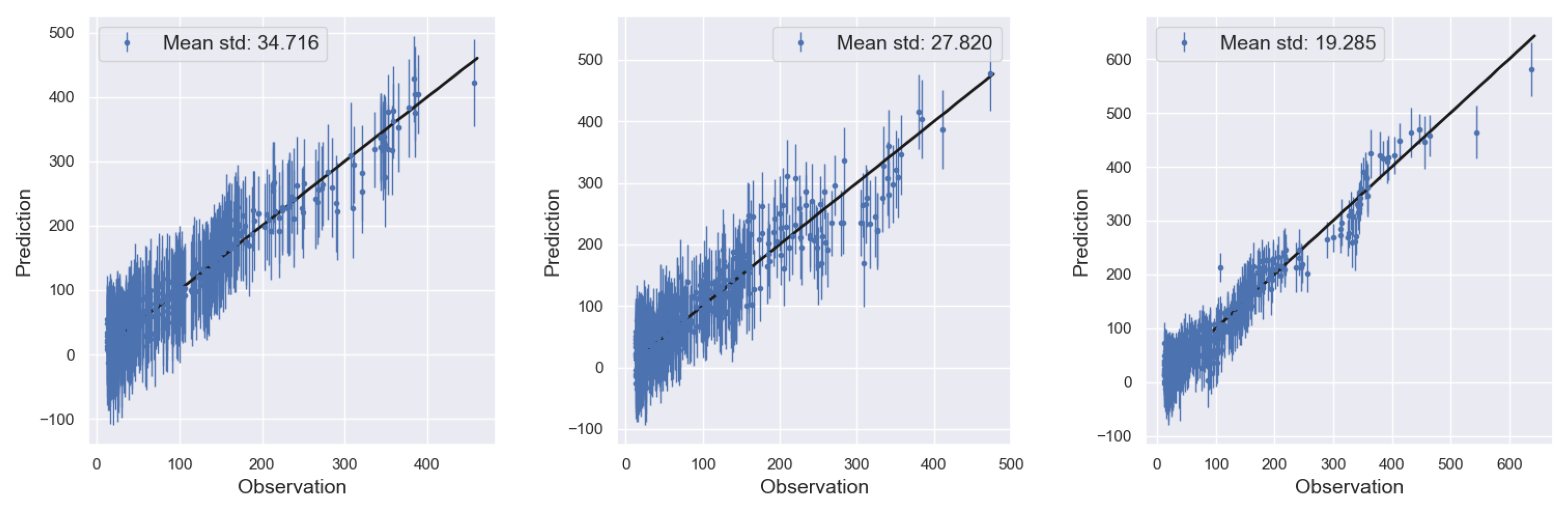
| N | Final | Mean Predictive Std | Runtime |
|---|---|---|---|
| 10 | 228.77 | 34.71 | 13’ |
| 50 | 265.64 | 27.82 | 61’ |
| 100 | 439.75 | 19.28 | 125’ |
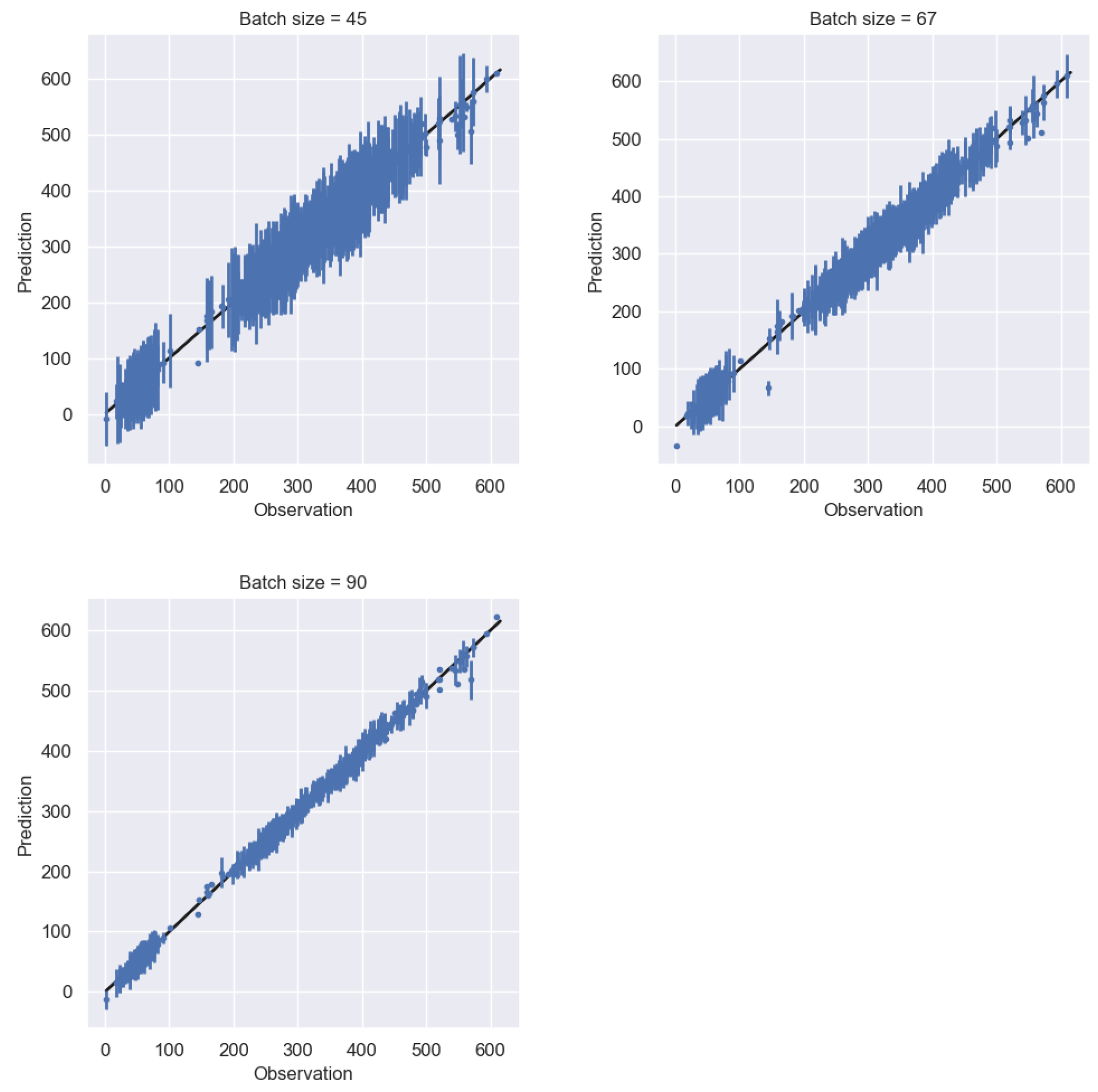
| Batch Size | RMSE Value | Mean Predictive Std |
|---|---|---|
| 45 | 6.445 | 24.626 |
| 67 | 6.315 | 15.065 |
| 90 | 5.254 | 7.889 |
| Part | Parameter | Value Range |
|---|---|---|
| Shaft 1 | Length | [9, 11] |
| Modulus of rigidity | [1053, 1287] | |
| Shaft 2 | Length | [10.8, 13.2] |
| Modulus of rigidity | [558, 682] | |
| Shaft 3 | Length | [7.2, 8.8] |
| Modulus of rigidity | [351, 429] | |
| Disk 1 | Diameter | [10.8, 13.2] |
| Thickness | [2.7, 3.3] | |
| Weight density | [0.252, 0.308] | |
| Disk 2 | Diameter | [12.6, 15.4] |
| Thickness | [3.6, 4.4] | |
| Weight density | [0.09, 0.11] |
| (Mean, Std) | (Mean, Std) | Runtime | |
|---|---|---|---|
| 50 | (0.092, 0.01) | (0.484, 0.042) | 9.7’ |
| 100 | (0.091, 0.01) | (0.487, 0.111) | 12.9’ |
| 150 | (0.132, 0.03) | (0.682, 0.179) | 14.1’ |
| 200 | (0.145, 0.27) | (0.554, 1.614) | 44.6’ |
| 250 | (0.088, 0.0008) | (0.450, 0.0007) | 54.4’ |
Publisher’s Note: MDPI stays neutral with regard to jurisdictional claims in published maps and institutional affiliations. |
© 2022 by the authors. Licensee MDPI, Basel, Switzerland. This article is an open access article distributed under the terms and conditions of the Creative Commons Attribution (CC BY) license (https://creativecommons.org/licenses/by/4.0/).
Share and Cite
Tsilifis, P.; Pandita, P.; Ghosh, S.; Wang, L. Multifidelity Model Calibration in Structural Dynamics Using Stochastic Variational Inference on Manifolds. Entropy 2022, 24, 1291. https://doi.org/10.3390/e24091291
Tsilifis P, Pandita P, Ghosh S, Wang L. Multifidelity Model Calibration in Structural Dynamics Using Stochastic Variational Inference on Manifolds. Entropy. 2022; 24(9):1291. https://doi.org/10.3390/e24091291
Chicago/Turabian StyleTsilifis, Panagiotis, Piyush Pandita, Sayan Ghosh, and Liping Wang. 2022. "Multifidelity Model Calibration in Structural Dynamics Using Stochastic Variational Inference on Manifolds" Entropy 24, no. 9: 1291. https://doi.org/10.3390/e24091291
APA StyleTsilifis, P., Pandita, P., Ghosh, S., & Wang, L. (2022). Multifidelity Model Calibration in Structural Dynamics Using Stochastic Variational Inference on Manifolds. Entropy, 24(9), 1291. https://doi.org/10.3390/e24091291