
Recognition of Vehicles Entering Expressway Service Areas and Estimation of Dwell Time Using ETC Data


Abstract
1. Introduction
- We proposed a VR-XGBoost model for recognizing vehicles entering expressway service areas based on ETC data, which not only achieves an effective estimation of the pause rate but also accurately recognizes individual vehicles driving into ESA.
- Taking into full consideration the driving pattern of vehicles entering/exiting the ESA, we proposed a K-VDTE model for vehicle dwell time estimation.
- The validity of the proposed method is verified by using real ETC data, which can provide a more scientific and reasonable reference basis for ESA reconstruction and extension.
2. Related Work
2.1. Pause Rate Estimation
2.2. Vehicle Dwell Time Estimation
3. Methodology
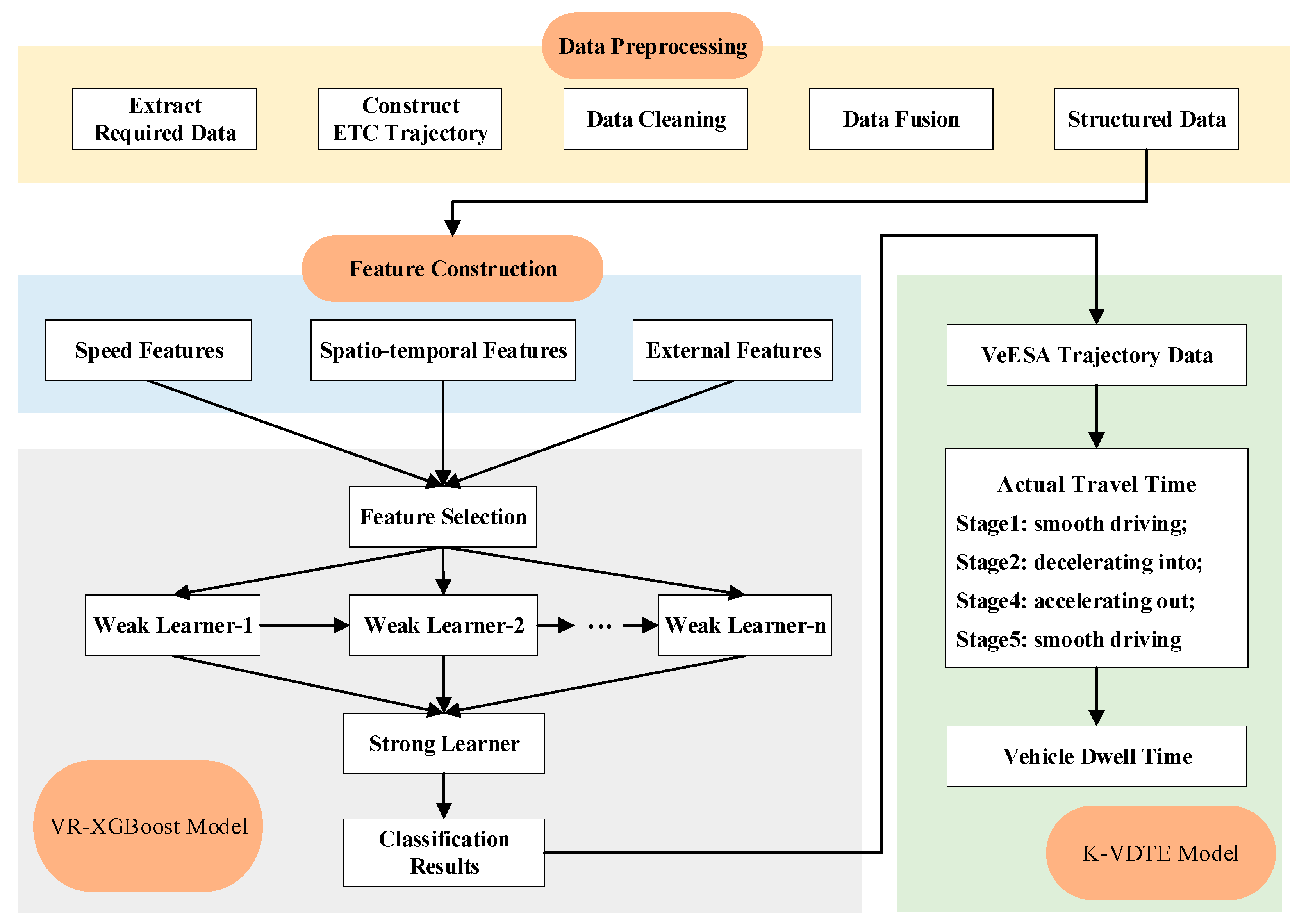
3.1. Framework
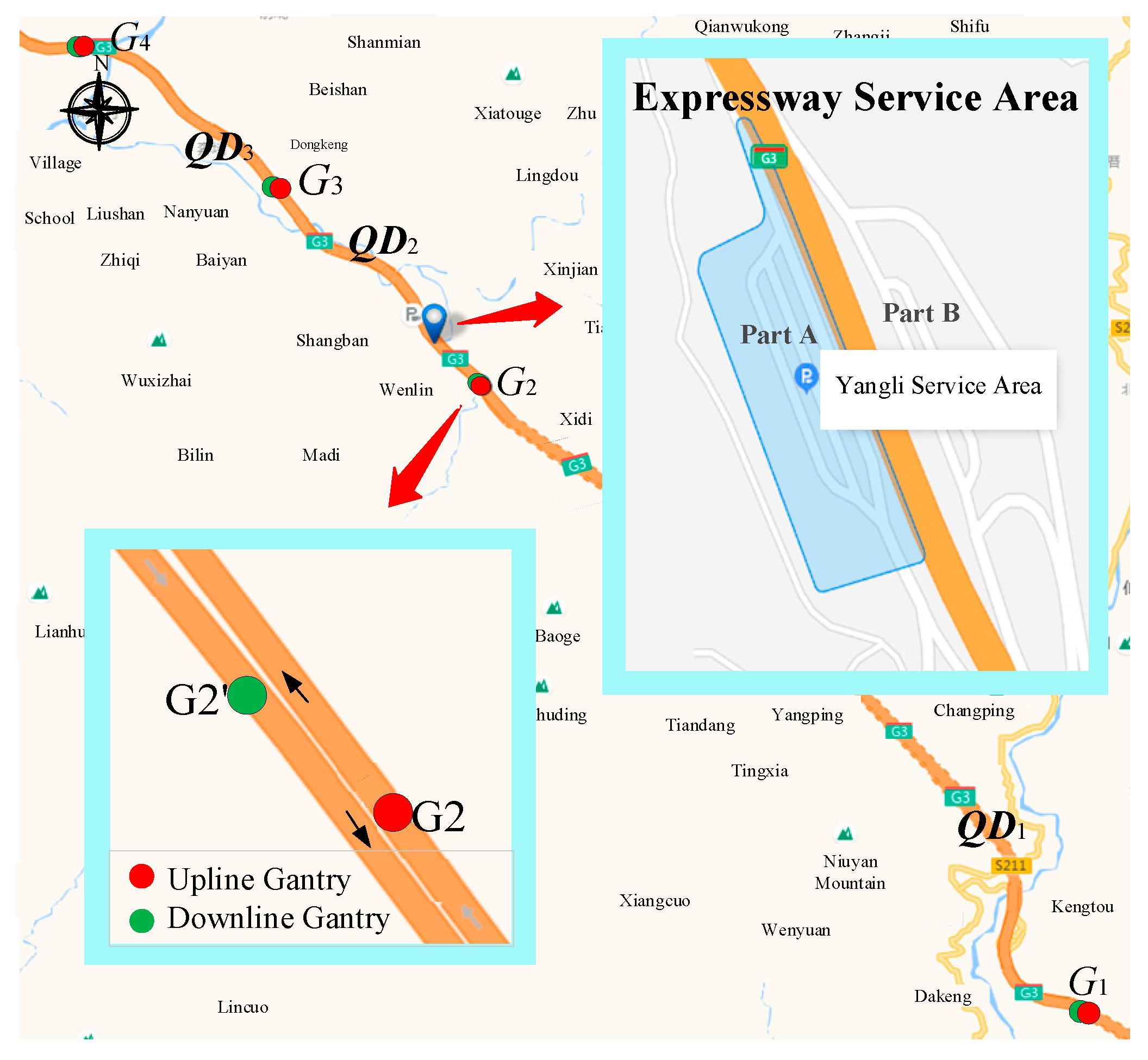
3.2. Data Overview and Preprocessing
3.2.1. Data Overview
3.2.2. Data Preprocessing
- (1)
- Data Redundancy
- (2)
- Data Missing
- (3)
- Data Abnormality
| Algorithm 1: ETC data cleaning algorithm |
| Input: ETC data eData, Topology data TP, Opposite topology data TP′ Output: ETC trajectory dataset 1: G_eData = eData.Groupby([,,]); # Grouping 2: For ∈ G_eData do: # Traversal operation for each set of data 3: # Sorted by transaction time 4: # Data deduplication 5: While (i=1, i < len()): 6: 7: IF : 8: 9: continue; 10: Else IF : 11: 12: 13: delete # Delete opposite gantry transaction data 14: i+= 2; 15: 16: , 17: IF && : 18: # Replacement of opposite gantry ID 19: i+= 2; 20: Else: 21: break; 22: End IF 23: End IF 24: Else: 25: break; 26: End IF 27: IF i = len()-1: 28: ; 29: End IF 30: End While 31: End For |
| Algorithm 2: Fusion of ETC trajectory and ESA data |
| Input: ETC trajectory dataset eTRAJ, ESA dataset sData, time difference ∆t Output: final trajectory data 1: 2: For do: 3: 4: 5: If in 6: s 7: For row in sdTmp.iterrows(): 8: IF < row.CapTime < : 9: ; 10: IF row.ExEn = 0: 11: 12: Else: 13: 14: End IF 15: Else: 16: continue; 17: End IF 18: End For 19: Else: 20: continue; 21: End IF 22: 23: End For |
3.3. XGBoost-Based VeESA Recognition
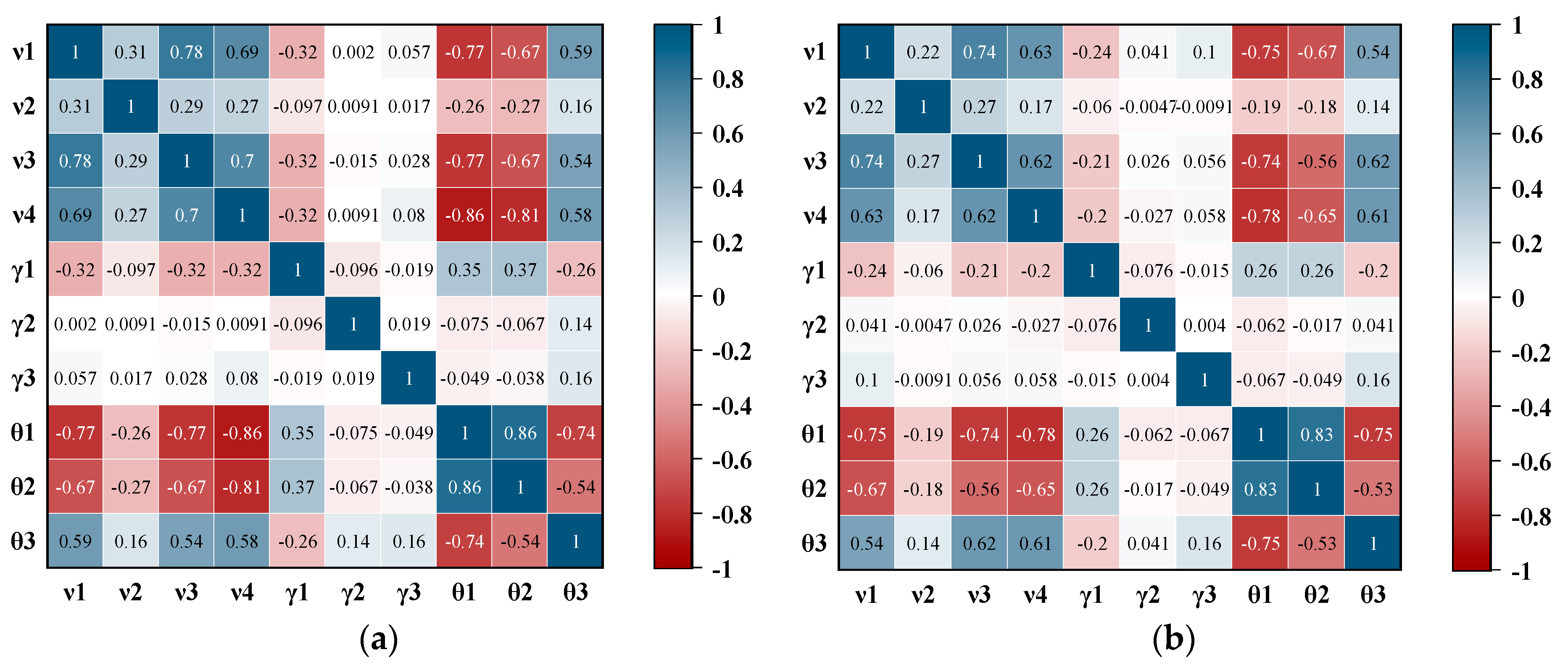
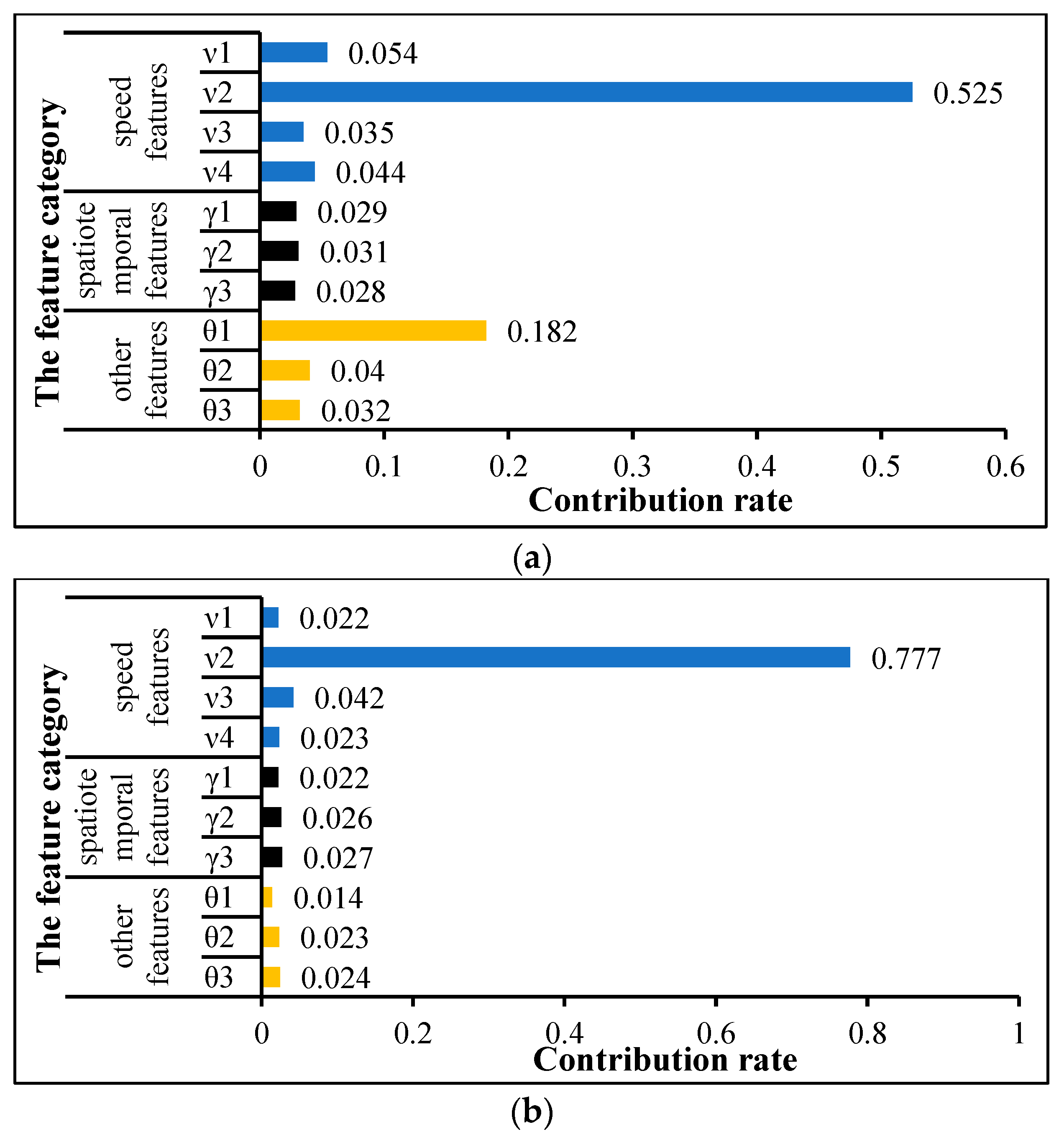
3.3.1. Feature Vector Modeling
- (1)
- Speed Features
- (2)
- Spatiotemporal Features
- (3)
- External Features
3.3.2. Modeling of Recognition of VeESA
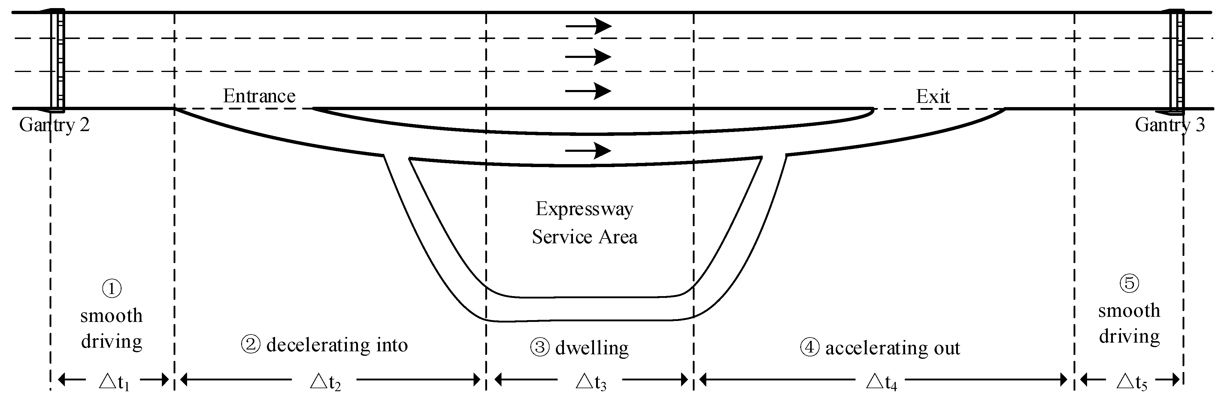
3.4. Kinematics-Based Dwell Time Estimation
- Stage 1: smooth driving upstream
- Stage 2: decelerating into the ESA
- Stage 4: accelerating out of the ESA
- Stage 5: smooth driving downstream
4. Experiments
4.1. VR-XGBoost Evaluation
4.1.1. Construction of Feature Vector
4.1.2. Parameters Selection
- (1)
- General Parameters: booster, silent, nthread, etc.
- (2)
- Booster Parameters: the number of decision trees (n_estimators), learning rate (learn_rate), maximum depth of the tree (max_depth), minimum weight in leaf nodes (min_child_weight), parameter that controls the number of leaves (gamma), proportion of sample sampling (subsample), scale of feature sampling (colsample_bytree), etc.
- (3)
- Learning Task Parameters: objective and evaluative (eval_metric).
4.1.3. Comparative Analysis of Classification Models
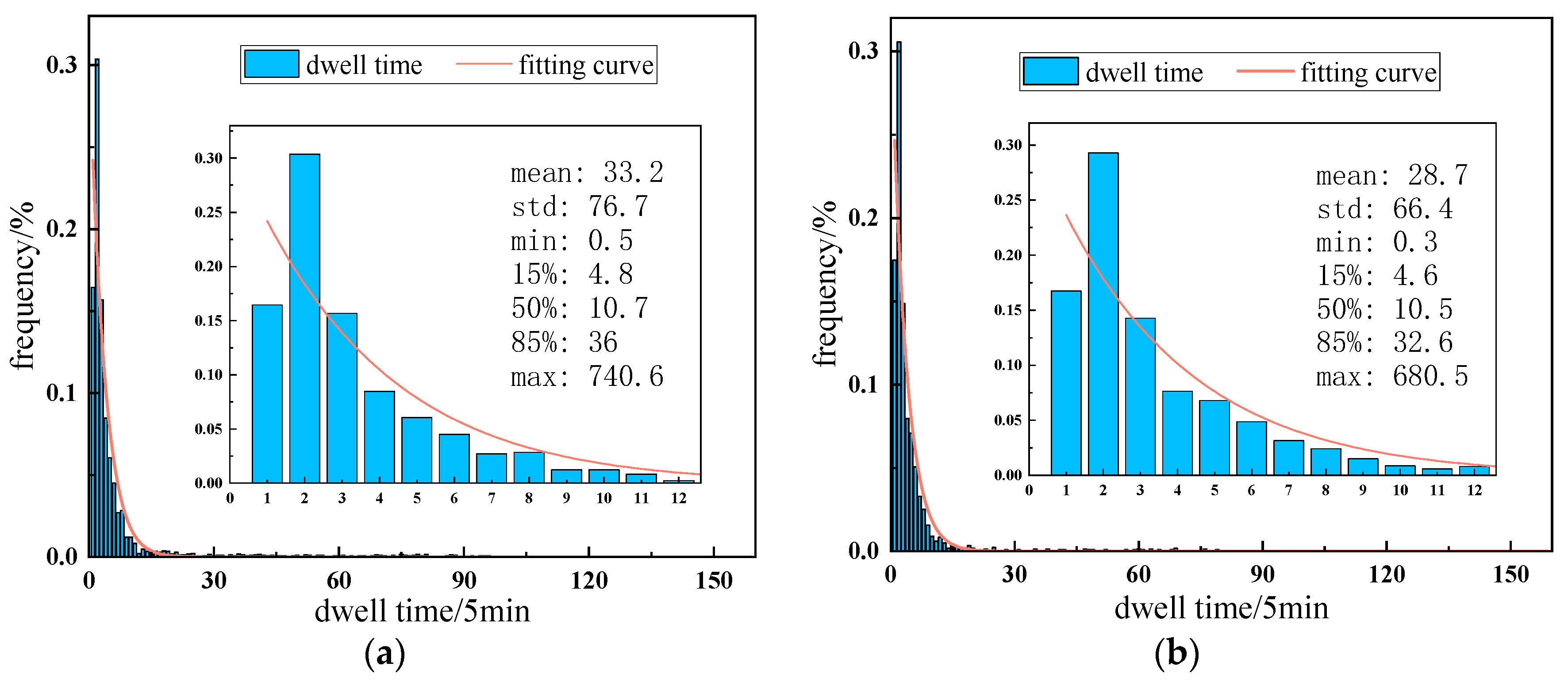
4.2. K-VDTE Evaluation
5. Conclusions
- (1)
- Experiments were conducted using real ETC data with a user penetration rate of over 80%. It not only solves the issue of insufficient data volume but also solves the geographical differences existing in different service areas in vehicle dwell time estimation. It can provide a more scientific and reasonable reference basis for the evaluation of the service capacity of ESA.
- (2)
- Considering multidimensional information such as speed features, spatiotemporal features and external features, we constructed a VR-XGBoost model. This model can achieve not only the estimation of the overall pause rate of ESA but also the accurate recognition of vehicles entering the service area.
- (3)
- After an in-depth study of the driving pattern of vehicles in the process of driving in/out of the ESA, we proposed a K-VDTE to realize vehicle dwell time estimation. The estimation accuracy of vehicle dwell time can be further improved by considering vehicle kinematics.
Author Contributions
Funding
Institutional Review Board Statement
Informed Consent Statement
Data Availability Statement
Conflicts of Interest
References
- Ministry of Transport of the Peoples’s Republic of China. 2021 Statistical Bulletin on the Development of the Transportation Industry; Ministry of Transport of the People’s Republic of China: Beijing, China, 2021.
- Hernandes, S.; Poliak, M.; Poliaková, A. Draft of freight transport car parks facilities. Arch. Motoryz. 2019, 85, 41–47. [Google Scholar]
- Seya, H.; Zhang, J.; Chikaraishi, M.; Ying, J. Decisions on truck parking place and time on expressways: An analysis using digital tachograph data. Transportation 2020, 47, 555–583. [Google Scholar] [CrossRef]
- Alkhatni, F.; Ishak, S.; Milad, A. Characteristics and Potential Impacts of Rest Areas Proximate to Roadways: A Review. Open Transp. J. 2021, 15, 260–271. [Google Scholar] [CrossRef]
- Hao, S.; Yang, P.; He, Z. The Design and Implementation of Big Data Application Management Platform for Highway Service Areas, Proceedings of the International Conference on Cyber Security Intelligence and Analytics, Shanghai, China, 18–19 March 2022; Springer: Cham, Switzerland, 2022; pp. 158–164. [Google Scholar]
- Japan Highway Public Corporation. Japan Highway Design Essentials; Japan Highway Public Corporation: Tokyo, Japan, 1991. [Google Scholar]
- Sun, X. Investigation and prediction of highway service area occupancy rate in Guangdong Province. Guangdong Highw. Traffic 2002, 1, 50–52. [Google Scholar] [CrossRef]
- Cui, H.; Liu, K. A New Determine Method on Pause Rate in Expressway Service Area Based on Vehicle Continuous Travel Time. J. Hebei Univ. Technol. 2008, 37, 100–104. [Google Scholar]
- Wang, J.; Tang, Y. Transportation potential calculation model of pause rate in expressway service area. China J. Highw. Transp. 2008, 21, 109–114. [Google Scholar]
- Ramli, I.; Hassan, S.; Hainin, M. Parking demand analysis of rest and service area along expressway in southern region, Johor Malaysia. Malays. J. Civ. Eng. 2017, 29. [Google Scholar] [CrossRef]
- Chen, Y.; Wang, J. A Study on Forecast Method of Pause Rate in Expressway Service Area. In Proceedings of the 22nd COTA International Conference of Transportation Professionals (CICTP 2022), Changsha, China, 8–11 July 2022. [Google Scholar]
- Liu, J.; Shen, X.; Liu, H. Prediction Model for Percentage of Expressway Traffic Entering Rest Area Based on BP Neural Network. Highway 2012, 6, 164–168. [Google Scholar] [CrossRef]
- Shen, X.; Wang, L.; Liu, H.; Yang, J. Estimation of the percentage of mainline traffic entering rest area based on BP neural network. J. Appl. Sci. 2013, 13, 2632–2638. [Google Scholar] [CrossRef]
- Lu, C. Research on Reasonable Allocation of Service Facilities in Expressway Service Area. Master’s Thesis, Beijing Jiaotong University, Beijing, China, 2017. [Google Scholar]
- Shen, X.; Zhang, F.; Lv, H.; Liu, J.; Liu, H. Prediction of entering percentage into expressway service areas based on wavelet neural networks and genetic algorithms. IEEE Access 2019, 7, 54562–54574. [Google Scholar] [CrossRef]
- Sun, C.; Lyu, H.; Yang, R.; Wei, Z.; Hao, X.; Pei, L. Traffic volume prediction for highway service areas based on XGBoost model with improved particle swarm optimization. J. Beijing Jiaotong Univ. 2021, 45, 74–83. [Google Scholar]
- Wang, J.; Zhang, K.; Zhi, P.; Xi, G.; Tang, X.; Zhou, Q. Analysis and Prediction Transient Population in Expressway Service Area based Long Short-Term Memory. In Proceedings of the 2021 IEEE 23rd International Conference on High Performance Computing & Communications; 7th International Conference on Data Science & Systems; 19th International Conference on Smart City; 7th International Conference on Dependability in Sensor, Cloud & Big Data Systems & Application (HPCC/DSS/SmartCity/DependSys), Haikou, China, 20–22 December 2021; pp. 1828–1832. [Google Scholar]
- Zhao, J.; Yu, Z.; Yang, X.; Gao, Z.; Liu, W. Short term traffic flow prediction of expressway service area based on STL-OMS. Phys. A Stat. Mech. Its Appl. 2022, 595, 126937. [Google Scholar] [CrossRef]
- King, G. NCHRP Report 324: Evaluation of Safety Roadside Rest Areas; TRB, National Research Council: Washington, DC, USA, 1989. [Google Scholar]
- Expressway Technical Research Institute. Expressway Traffic Statistics Data Book; Expressway Technical Research Institute: Machida, Japan, 2014; pp. 166–185. [Google Scholar]
- Umayahara, A.; Akagi, T.; Suzuki, H. Study on The State of Rest Behavior at Expressway Rest Areas. J. Archit. Plan. (Trans. AIJ) 2017, 82, 1639–1647. [Google Scholar] [CrossRef]
- Perfater, M. Operation and motorist usage of interstate rest areas and welcome centers in Virginia. Transp. Res. Rec. 1989, 1224, 46–53. [Google Scholar]
- Twardzik, L.; Haskell, T. Rest Area/Roadside Park Administration, Use and Operations; Michigan State University: Lansing, MI, USA, 1985. [Google Scholar]
- Al-Kaisy, A.; Church, B.; Veneziano, D.; Dorrington, C. Investigation of Parking Dwell Time at Rest Areas on Rural Highways. Transp. Res. Rec. 2011, 2255, 156–164. [Google Scholar] [CrossRef]
- Li, Z.; Miao, Q.; Shehzad, A.; Chen, C. A provably secure and lightweight mutual authentication protocol in fog-enabled social Internet of vehicles. Int. J. Distrib. Sens. Netw. 2022, 18, 15501329221104332. [Google Scholar] [CrossRef]
- Wu, J.; Wei, M.; Srivastava, G.; Chen, C.; Lin, J. Mining large-scale high utility patterns in vehicular ad hoc network environments. Trans. Emerg. Telecommun. Technol. 2020. [Google Scholar] [CrossRef]
- Liao, L.; Lin, J.; Zhu, Y.; Bi, S.; Lin, Y. A Bi-direction LSTM Attention Fusion Model for the Missing POI Identification. J. Netw. Intell. 2022, 7, 161–174. [Google Scholar]
- He, Y.; Qin, Q.; Josef, V. A pedestrian detection method using SVM and CNN multistage classification. J. Inf. Hiding Multimed. Signal Process. 2018, 9, 51–60. [Google Scholar]
- Hirai, S.; Xing, J.; Kobayashi, M.; Ryota, H.; Nobuhiro, U. Preliminary analysis on the resting behavior of expressway users with ETC data. In Proceedings of the 22nd ITS World Congress, Bordeaux, France, 5–9 October 2015. [Google Scholar]
- Hirai, S.; Xing, J.; Kai, S.; Ryota, H.; Nobuhiro, U. Study of resting behavior on inter-urban expressways using ETC 2.0 probe data. In Proceedings of the 23rd ITS World Congress, Melbourne, Australia, 10–14 October 2016; pp. 10–14. [Google Scholar]
- Muramatsu, T.; Oguchi, T. Proposal and application of parking area performance measurement methodology. Transp. Res. Procedia 2016, 15, 628–639. [Google Scholar] [CrossRef][Green Version]
- Jin, S. Study of the Forecast for the Volume of Freight Handled in Freeway Service Area. Sci. Technol. Eng. 2008, 8, 3233–3237. [Google Scholar]
- Choe, Y.; Baek, S. A Study on Proper Size of Expressway Service Area. J. Korean Soc. Transp. 2009, 27, 7–18. [Google Scholar]
- Kim, J.; Yang, T.; Yoon, T. Evaluation of Current Service Areas’ Location to Improve Freight Car’s Safety: A Case Study of Seohaean Expressway. J. Korean Soc. Transp. 2020, 38, 335–345. [Google Scholar] [CrossRef]
- Tint, T.; Maung, H.; Wyityi, W. Comparative Analysis on Highway Rest Centers along Yangon-Mandalay Expressway. Int. J. Emerg. Technol. Adv. Eng. 2013, 3, 41–48. [Google Scholar]
- Wang, S.; Xu, Y. Calculation of reasonable scale of parking spaces in expressway service area based on queuing theory. J. Highw. Transp. Res. Dev. 2016, 3, 116–119. [Google Scholar]
- Kumar, V.; Kumar, R.; Jangirala, S.; Kumari, S.; Kumar, S.; Chen, C. An enhanced RFID-based authentication protocol using PUF for vehicular cloud computing. Secur. Commun. Netw. 2022, 2022, 8998339. [Google Scholar] [CrossRef]
- Liu, L.; He, D.; Ma, Y.; Zhang, X.; Huang, J.; Li, J.; Yao, J. A novel license plate location method based on deep learning. J. Netw. Intell. 2020, 5, 93–101. [Google Scholar]
- Luo, S.; Zou, F.; Zhang, C.; Tian, J.; Guo, F.; Liao, L. Multi-View Travel Time Prediction Based on Electronic Toll Collection Data. Entropy 2022, 24, 1050. [Google Scholar] [CrossRef]
- Khanh, H.N. Classification of Concepts Using Decision Trees for Inconsistent Knowledge Systems Based on Bisimulation. J. Inf. Hiding Multimed. Signal Process. 2021, 12, 22–30. [Google Scholar]
- Zhi, Y.; Zhang, J.; Shi, Z. Research on Design of Expressway Acceleration Lane Length and Merging Model of Vehicle. China J. Highw. Transp. 2009, 22, 93–97+115. [Google Scholar]
- Zou, F.; Guo, F.; Tian, J.; Luo, S.; Yu, X.; Gu, Q.; Liao, L. The Method of Dynamic Identification of the Maximum Speed Limit of Expressway Based on Electronic Toll Collection Data. Sci. Program. 2021, 2021, 4702669. [Google Scholar] [CrossRef]


| Field Name | Description | Example | |
|---|---|---|---|
| 1 | VehID | vehicle ID | A000001 |
| 2 | VehClass | vehicle type | 1 |
| 3 | EnWeight | entrance gross axle weight | 1500 |
| 4 | EnStation | entrance ID | 1002 |
| 5 | EnTime | entrance time | 2020/9/5 00:00:00 |
| 6 | GantryID | gantry ID | G000335001000120020 |
| 7 | TradeTime | transaction time | 2020/9/5 01:00:00 |
| 8 | Workday | workday | 0 |
| Field Name | Description | Example | |
|---|---|---|---|
| 1 | SAID | service area ID | Yangli Part A |
| 2 | EnEx | entrance/exit | 0/1 |
| 3 | VehID | vehicle ID | A000001 |
| 4 | CapTime | capture time | 2020/9/5 00:00:00 |
| Part A | A0000001 | 2020-09-05 08:06:03 | 2020-09-05 08:08:20 | 2020-09-05 08:14:12 | 2020-09-05 08:23:02 | 23 | 6101 | 2020-09-05 06:29:55 | 18.8 | 1 | 2020-09-05 08:01:59 | 2020-09-05 08:04:08 | 1 |
| A0000002 | 2020-09-03 06:28:34 | 2020-09-03 06:30:46 | 2020-09-03 06:43:52 | 2020-09-03 06:52:07 | 22 | 6103 | 2020-09-03 04:24:28 | 11.4 | 0 | 2020-09-03 06:24:42 | 2020-09-03 06:33:32 | 1 | |
| A0000003 | 2020-09-10 23:38:27 | 2020-09-10 23:40:24 | 2020-09-10 23:43:03 | 2020-09-10 23:50:57 | 1 | 2202 | 2020-09-10 23:19:23 | 0 | 0 | 0 | |||
| A0000004 | 2020-09-07 03:51:13 | 2020-09-07 03:54:27 | 2020-09-07 03:59:52 | 2020-09-07 04:11:46 | 11 | 6101 | 2020-09-06 22:46:11 | 14.3 | 0 | 0 | |||
| A0000005 | 2020-09-03 21:14:13 | 2020-09-03 21:17:24 | 2020-09-04 04:56:05 | 2020-09-04 05:06:41 | 16 | 6307 | 2020-09-03 19:33:43 | 45.1 | 0 | 2020-09-03 21:12:24 | 1 | ||
| Part B | A0000006 | 2020-09-04 17:17:52 | 2020-09-04 17:32:36 | 2020-09-04 17:48:00 | 2020-09-04 17:50:17 | 16 | 6707 | 2020-09-04 16:48:35 | 50.1 | 0 | 2020-09-04 17:36:41 | 1 | |
| A0000007 | 2020-09-08 13:42:53 | 2020-09-08 13:54:00 | 2020-09-08 14:05:48 | 2020-09-08 14:07:57 | 2 | 6707 | 2020-09-08 13:23:20 | 0 | 0 | 0 | |||
| A0000008 | 2020-09-06 10:47:19 | 2020-09-06 10:55:17 | 2020-09-06 11:19:16 | 2020-09-06 11:21:21 | 3 | 2903 | 2020-09-06 09:52:21 | 0 | 1 | 2020-09-06 10:47:21 | 2020-09-06 11:08:32 | 1 | |
| A0000009 | 2020-09-06 16:58:22 | 2020-09-06 17:07:12 | 2020-09-06 17:09:52 | 2020-09-06 17:12:13 | 12 | 6707 | 2020-09-06 16:37:20 | 7.6 | 1 | 0 | |||
| A0000010 | 2020-09-10 21:51:28 | 2020-09-10 22:01:59 | 2020-09-10 22:21:59 | 2020-09-10 22:24:20 | 14 | 6707 | 2020-09-10 21:25:11 | 17.9 | 0 | 2020-09-10 21:53:26 | 2020-09-10 22:09:52 | 1 |
| Part A | 114.6 | 21.4 | 109.2 | 85.7 | 0.88 | 14 | 0 | 2 | 0 | 4 | 1 |
| 92.0 | 93.4 | 84.9 | 92.1 | 1.01 | 10 | 0 | 2 | 0 | 3 | 0 | |
| 68.0 | 7.2 | 66.6 | 54.1 | 12.18 | 21 | 1 | 13 | 13.54 | 10 | 1 | |
| 75.4 | 69.6 | 69.3 | 48.6 | 1.86 | 21 | 0 | 14 | 15.9 | 11 | 0 | |
| 77.4 | 60.5 | 64.8 | 44.9 | 18.55 | 22 | 1 | 15 | 30.28 | 8 | 0 | |
| 70.0 | 64.4 | 77.8 | 68.4 | 2.72 | 15 | 0 | 21 | 0 | 4 | 0 | |
| Part B | 67.6 | 21.2 | 79.6 | 84.1 | 0.81 | 17 | 0 | 12 | 9.3 | 6 | 1 |
| 80.4 | 88.3 | 81.3 | 83.8 | 0.73 | 18 | 1 | 12 | 7.5 | 8 | 0 | |
| 77.0 | 20.1 | 86.1 | 74.4 | 0.56 | 20 | 0 | 11 | 4.6 | 16 | 1 | |
| 67.1 | 76.2 | 72.2 | 66.3 | 0.81 | 21 | 0 | 11 | 0 | 22 | 0 | |
| 90.1 | 9.7 | 104.7 | 94.9 | 0.42 | 22 | 1 | 1 | 0 | 69 | 1 | |
| 91.6 | 102.5 | 99.3 | 96.7 | 2.35 | 23 | 0 | 1 | 0 | 20 | 0 |
| Parameter | Search Range | Step Size | Optimal Value | |
|---|---|---|---|---|
| General Parameters | booster | gbtree/gblinear | gbtree | |
| silent | 0/1 | 0 | ||
| nthread | 4 | |||
| Booster Parameters | n_estimators | [100, 1000] | 100 | 300 |
| learn_rate | [0, 0.5] | 0.01 | 0.1 | |
| max_depth | [1, 10] | 1 | 5 | |
| min_child_weight | [1, 10] | 1 | 1 | |
| gamma | [0, 0.5] | 0.1 | 0 | |
| subsample | [0.6, 1] | 0.05 | 0.8 | |
| colsample_bytree | [0.6, 1] | 0.05 | 0.8 | |
| Learning Task Parameters | objective | reg:linear/reg:logistic/ binary:logistic/… | binary:logistic | |
| eval_metric | error/auc/rmse/… | auc |
| Model | Part A | Part B | ||||||
|---|---|---|---|---|---|---|---|---|
| Accuracy | Precision | Recall | F1-Score | Accuracy | Precision | Recall | F1-Score | |
| GaussianNB | 0.937 | 0.94 | 0.937 | 0.937 | 0.962 | 0.962 | 0.962 | 0.962 |
| SVM | 0.954 | 0.954 | 0.954 | 0.954 | 0.973 | 0.974 | 0.973 | 0.973 |
| KNN | 0.955 | 0.956 | 0.955 | 0.955 | 0.973 | 0.974 | 0.973 | 0.973 |
| DT | 0.913 | 0.914 | 0.914 | 0.914 | 0.947 | 0.947 | 0.947 | 0.947 |
| AdaBoost | 0.941 | 0.942 | 0.941 | 0.941 | 0.969 | 0.97 | 0.969 | 0.969 |
| LR | 0.947 | 0.947 | 0.947 | 0.947 | 0.966 | 0.966 | 0.966 | 0.966 |
| RF | 0.958 | 0.96 | 0.958 | 0.958 | 0.973 | 0.974 | 0.973 | 0.973 |
| GBDT | 0.958 | 0.959 | 0.958 | 0.958 | 0.973 | 0.974 | 0.973 | 0.973 |
| VR-XGBoost | 0.959 | 0.96 | 0.959 | 0.959 | 0.974 | 0.974 | 0.974 | 0.974 |
| Model | Part A | Part B | ||||
|---|---|---|---|---|---|---|
| RMSE | MAE | RMSE | MAE | |||
| Lasso | 4046 | 2095 | 0.275 | 3831 | 1823 | 0.2 |
| KNN | 3443 | 1148 | 0.475 | 3506 | 1073 | 0.33 |
| AdaBoost | 536 | 431 | 0.987 | 486 | 400 | 0.987 |
| DT | 318 | 90 | 0.995 | 263 | 65 | 0.996 |
| ExtraTree | 365 | 92 | 0.994 | 1248 | 146 | 0.915 |
| RF | 276 | 71 | 0.997 | 263 | 55 | 0.996 |
| GBDT | 272 | 72 | 0.997 | 315 | 61 | 0.994 |
| XGBoost | 242 | 70 | 0.997 | 263 | 62 | 0.996 |
| AvgSpeed | 85 | 71 | 1.000 | 36 | 30 | 1.000 |
| K-VDTE | 69 | 52 | 1.000 | 22 | 14 | 1.000 |
Publisher’s Note: MDPI stays neutral with regard to jurisdictional claims in published maps and institutional affiliations. |
© 2022 by the authors. Licensee MDPI, Basel, Switzerland. This article is an open access article distributed under the terms and conditions of the Creative Commons Attribution (CC BY) license (https://creativecommons.org/licenses/by/4.0/).
Share and Cite
Cai, Q.; Yi, D.; Zou, F.; Zhou, Z.; Li, N.; Guo, F. Recognition of Vehicles Entering Expressway Service Areas and Estimation of Dwell Time Using ETC Data. Entropy 2022, 24, 1208. https://doi.org/10.3390/e24091208
Cai Q, Yi D, Zou F, Zhou Z, Li N, Guo F. Recognition of Vehicles Entering Expressway Service Areas and Estimation of Dwell Time Using ETC Data. Entropy. 2022; 24(9):1208. https://doi.org/10.3390/e24091208
Chicago/Turabian StyleCai, Qiqin, Dingrong Yi, Fumin Zou, Zhaoyi Zhou, Nan Li, and Feng Guo. 2022. "Recognition of Vehicles Entering Expressway Service Areas and Estimation of Dwell Time Using ETC Data" Entropy 24, no. 9: 1208. https://doi.org/10.3390/e24091208
APA StyleCai, Q., Yi, D., Zou, F., Zhou, Z., Li, N., & Guo, F. (2022). Recognition of Vehicles Entering Expressway Service Areas and Estimation of Dwell Time Using ETC Data. Entropy, 24(9), 1208. https://doi.org/10.3390/e24091208