
Quantum Statistical Complexity Measure as a Signaling of Correlation Transitions

 ,
,  , , , and
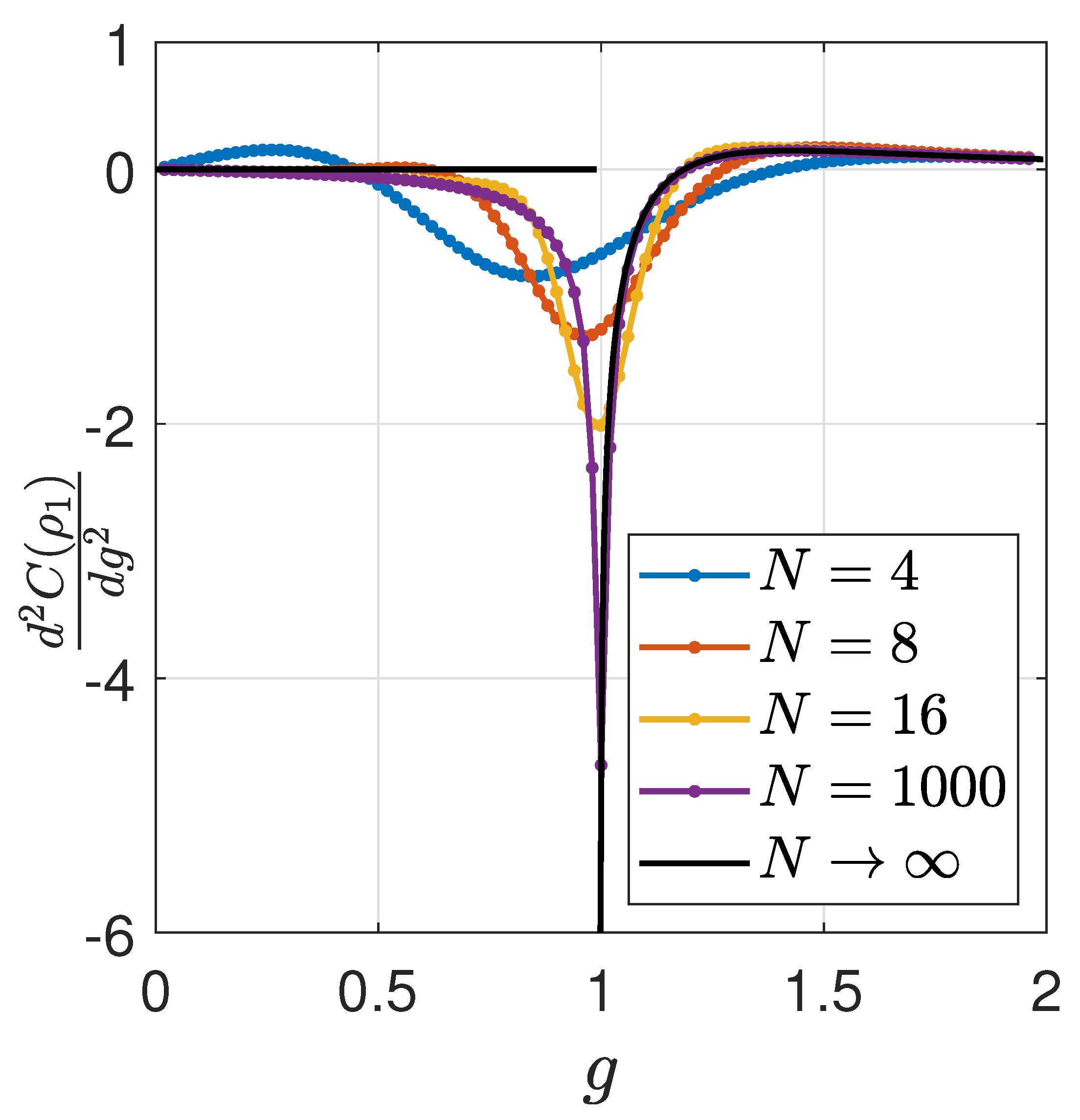
Abstract
1. Introduction
2. Classical Statistical Complexity Measure—CSCM
2.1. Degree of Order
2.2. Degree of Disorder
2.3. Quantifying Classical Complexity
3. Quantum Statistical Complexity Measure—QSCM
3.1. Quantifying Quantum Complexity
3.2. Some Properties of the QSCM
4. Examples and Applications
4.1. QSCM of One-Qubit
4.2. Quantum Ising Model
- A Jordan–Wigner transformation:where and are the annihilation-creation operators, respecting the anti-commutation relations: , and ;
- A Discrete Fourier Transform (DFT):
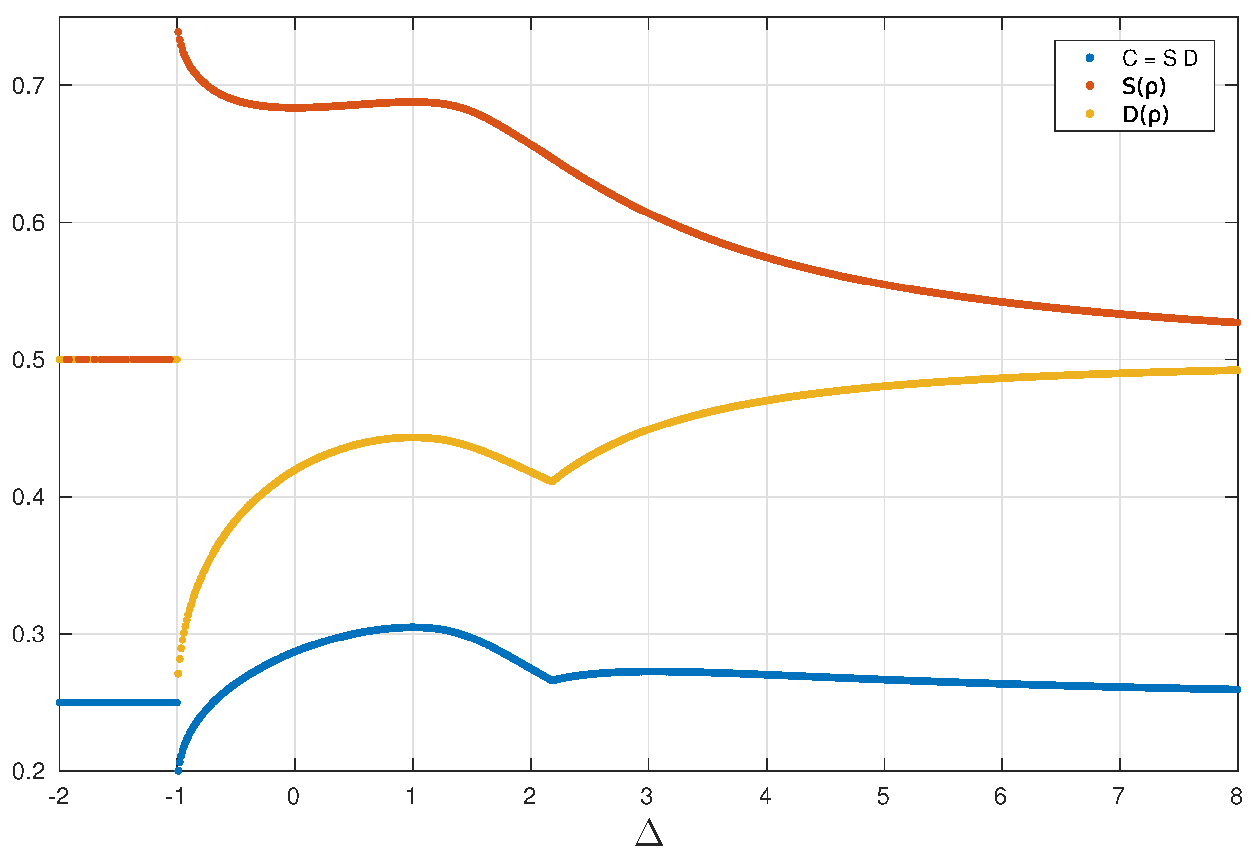
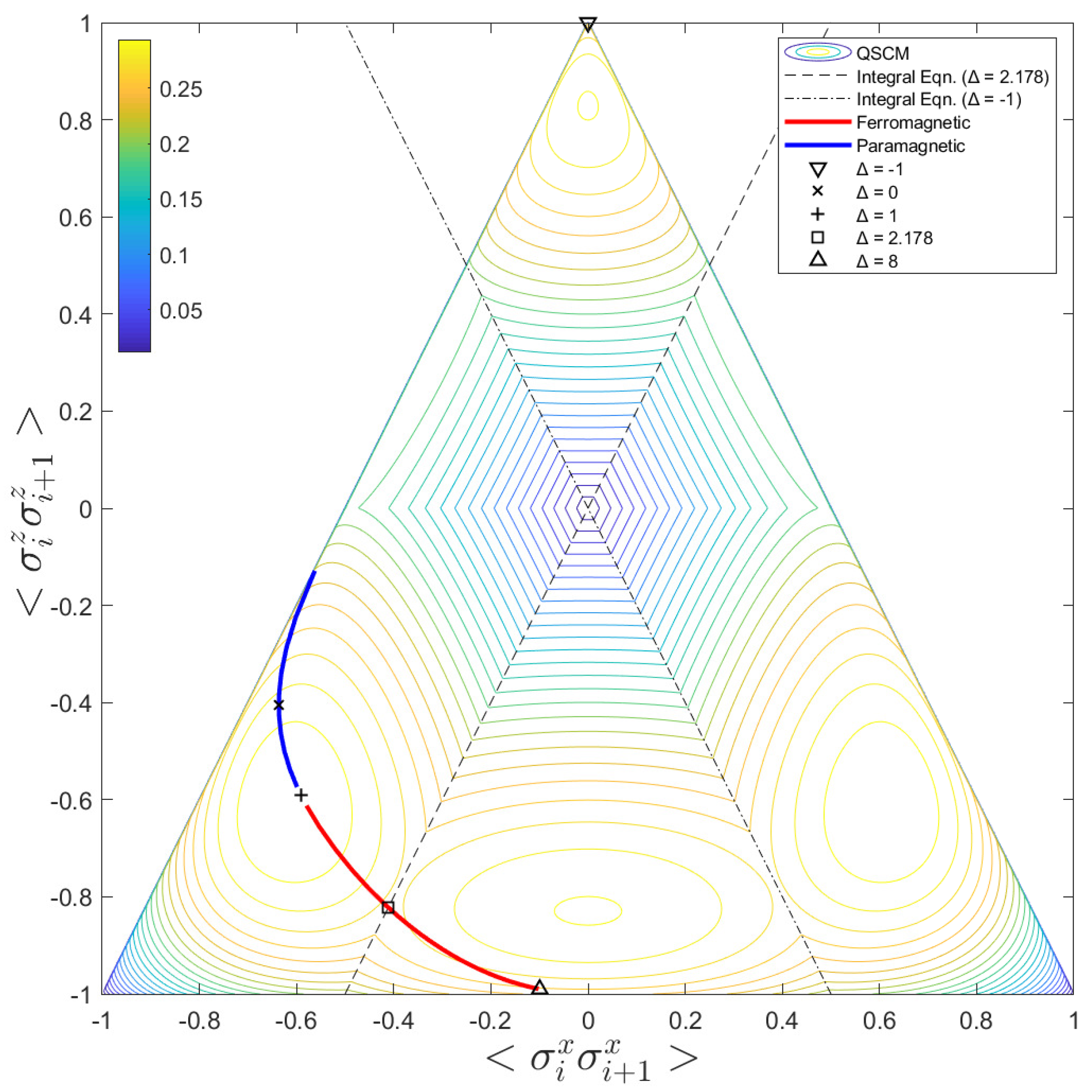
4.3. XXZ-½ Model
5. Conclusions
Author Contributions
Funding
Institutional Review Board Statement
Informed Consent Statement
Data Availability Statement
Acknowledgments
Conflicts of Interest
Abbreviations
| CSCM | Classical Statistical Complexity Measure |
| QSCM | Quantum Statistical Complexity Measure |
Appendix A. Sub-Additivity over Copies
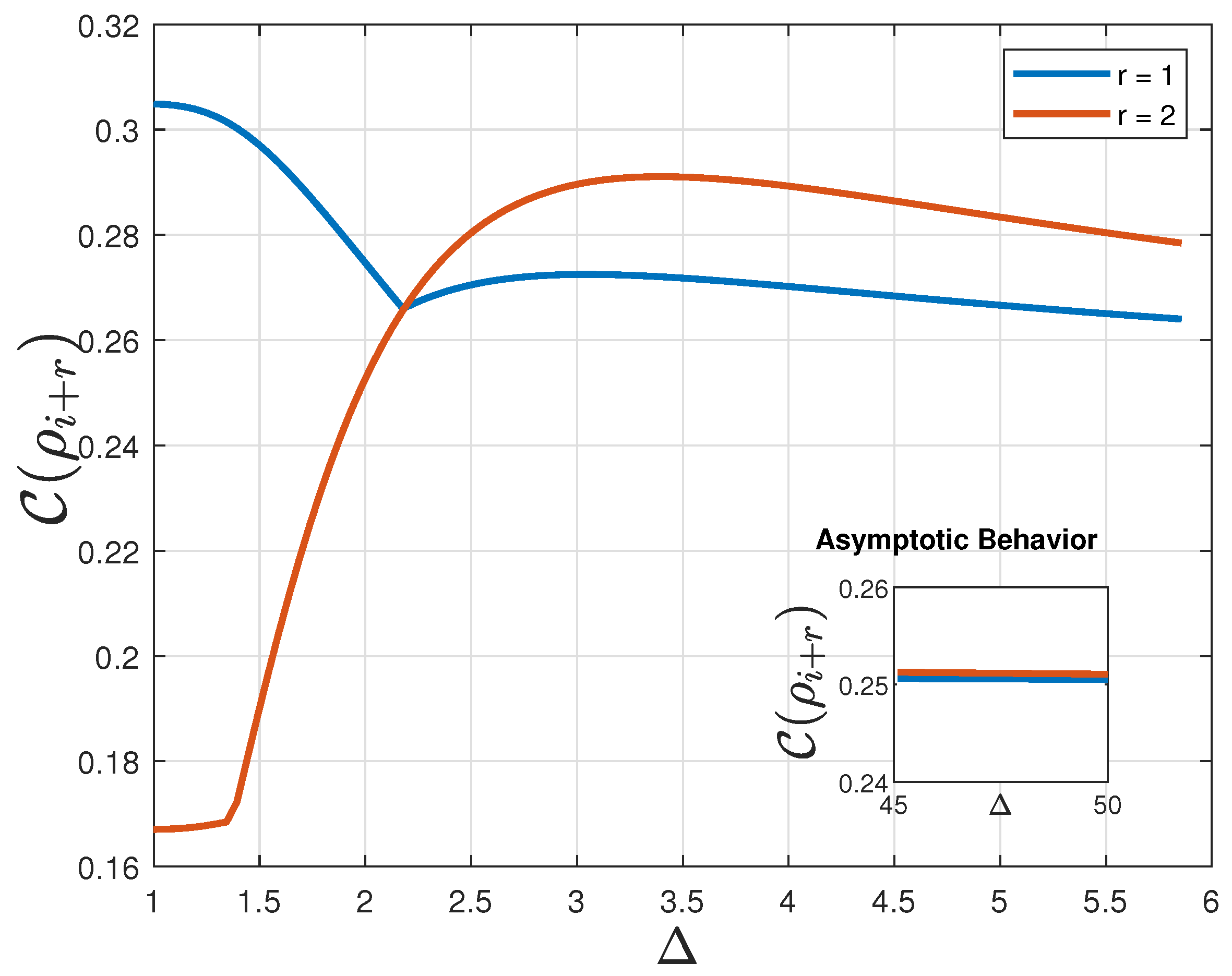
Appendix B. Correlation Functions for Nearest Neighbors and Next-to-Nearest Neighbors
References
- Badii, R.; Politi, A. Complexity: Hierarchical Structures and Scaling in Physics; Cambridge University Press: Cambridge, UK, 1997. [Google Scholar]
- Lempel, A.; Ziv, J. On the Complexity of Finite Sequences. IEEE Trans. Inf. Theory 1976, 22, 75–81. [Google Scholar] [CrossRef]
- Jiménez-Montaño, M.A.; Ebeling, W.; Pohl, T.; Rapp, P.E. Entropy and complexity of finite sequences as fluctuating quantities. Biosystems 2002, 64, 23–32. [Google Scholar] [CrossRef]
- Szczepanski, J. On the distribution function of the complexity of finite sequences. Inf. Sci. 2009, 179, 1217–1220. [Google Scholar] [CrossRef][Green Version]
- Kolmogorov, A.N. Three approaches to the quantitative definition of information. Probl. Inf. Transm. 1965, 1, 1–7. [Google Scholar] [CrossRef]
- Chaitin, G.J. On the Length of Programs for Computing Finite Binary Sequences. J. ACM 1966, 13, 547–569. [Google Scholar] [CrossRef]
- Martin, M.T.; Plastino, A.; Rosso, O.A. Statistical complexity and disequilibrium. Phys. Lett. A 2003, 311, 126–132. [Google Scholar] [CrossRef]
- Lamberti, P.W.; Martin, M.T.; Plastino, A.; Rosso, O.A. Intensive entropic non-triviality measure. Phys. A 2004, 334, 119–131. [Google Scholar] [CrossRef]
- Binder, P.-M. Complexity and Fisher information. Phys. Rev. E 2000, 61, R3303–R3305. [Google Scholar] [CrossRef] [PubMed]
- Shiner, J.S.; Davison, M.; Landsberg, P.T. Simple measure for complexity. Phys. Rev. E 1999, 59, 1459–1464. [Google Scholar] [CrossRef]
- Toranzo, I.V.; Dehesa, J.S. Entropy and complexity properties of the d-dimensional blackbody radiation. Eur. Phys. J. D 2014, 68, 316. [Google Scholar] [CrossRef]
- Wackerbauer, R.; Witt, A.; Atmanspacher, H.; Kurths, J.; Scheingraber, H. A comparative classification of complexity measures. Chaos Solitons Fractals 1994, 4, 133–173. [Google Scholar] [CrossRef]
- Zurek, W.H. Complexity, Entropy, and the Physics of Information; Addison-Wesley Pub. Co.: Redwood City, CA, USA, 1990. [Google Scholar]
- Domenico, F.; Stefano, M.; Nihat, A. Canonical Divergence for Measuring Classical and Quantum Complexity. Entropy 2019, 21, 435. [Google Scholar]
- Felice, D.; Cafaro, C.; Mancini, S. Information geometric methods for complexity. Chaos 2018, 28, 032101. [Google Scholar] [CrossRef] [PubMed]
- Crutchfield, J.P.; Ellison, C.J.; Mahoney, J.R. Time’s Barbed Arrow: Irreversibility, Crypticity, and Stored Information. Phys. Rev. Lett. 2009, 103, 94101. [Google Scholar] [CrossRef] [PubMed]
- Riechers, P.M.; Mahoney, J.R.; Aghamohammadi, C.; Crutchfield, J.P. Minimized state complexity of quantum-encoded cryptic processes. Phys. Rev. A 2016, 93, 052317. [Google Scholar] [CrossRef]
- Gu, M.; Wiesner, K.; Rieper, E.; Vedral, V. Quantum mechanics can reduce the complexity of classical models. Nat. Commun. 2012, 3, 762–765. [Google Scholar] [CrossRef] [PubMed]
- Yang, C.; Binder, F.C.; Narasimhachar, V.; Gu, M. Matrix Product States for Quantum Stochastic Modeling. Phys. Rev. Lett. 2018, 121, 260602. [Google Scholar] [CrossRef] [PubMed]
- Thompson, J.; Garner, A.J.P.; Mahoney, J.R.; Crutchfield, J.P.; Vedral, V.; Gu, M. Causal Asymmetry in a Quantum World. Phys. Rev. X 2018, 8, 031013. [Google Scholar] [CrossRef]
- López-Ruiz, R.; Mancini, H.L.; Calbet, X. A statistical measure of complexity. Phys. Lett. A 1995, 209, 321–326. [Google Scholar] [CrossRef]
- Anteneodo, C.; Plastino, A.R. Some features of the López-Ruiz-Mancini-Calbet (LMC) statistical measure of complexity. Phys. Lett. A 1996, 223, 348–354. [Google Scholar] [CrossRef]
- Catalán, R.G.; Garay, J.; López-Ruiz, R. Features of the extension of a statistical measure of complexity to continuous systems. Phys. Rev. E 2002, 66, 011102. [Google Scholar] [CrossRef] [PubMed]
- Rosso, O.A.; Martin, M.T.; Larrondo, H.A.; Kowalski, A.M.; Plastino, A. Generalized Statistical Complexity—A New Tool for Dynamical Systems; Bentham Science Publisher: Sharjah, United Arab Emirates, 2013. [Google Scholar]
- Tsallis, C. Possible generalization of Boltzmann-Gibbs statistics. J. Stat. Phys. 1988, 52, 479–487. [Google Scholar] [CrossRef]
- Gell-Mann, M.; Tsallis, C. Nonextensive Entropy-Interdisciplinary Applications; Oxford University Press: Oxford, UK, 2004. [Google Scholar]
- Rényi, A. On measures of Entropy and Information; University of California Press: Berkeley, CA, USA, 1961; pp. 547–561. [Google Scholar]
- Bhattacharyya, A. On a Measure of Divergence between Two Statistical Populations Defined by Their Probability Distributions. Bull. Calcutta Math. Soc. 1943, 35, 99–109. [Google Scholar]
- Majtey, A.; Lamberti, P.W.; Martin, M.T.; Plastino, A. Wootters’ distance revisited: A new distinguishability criterium. Eur. Phys. J. D 2005, 32, 413–419. [Google Scholar] [CrossRef]
- Kullback, S.; Leibler, R.A. On Information and Sufficiency. Ann. Math. Stat. 1951, 22, 79–86. [Google Scholar] [CrossRef]
- Majtey, A.P.; Lamberti, P.W.; Prato, D.P. Jensen-Shannon divergence as a measure of distinguishability between mixed quantum states. Phys. Rev. A 2005, 72, 052310. [Google Scholar] [CrossRef]
- López-Ruiz, R.; Nagy, Á.; Romera, E.; Sañudo, J. A generalized statistical complexity measure: Applications to quantum systems. J. Math. Phys. 2009, 50, 123528. [Google Scholar] [CrossRef]
- Sañudo, J.; López-Ruiz, R. Statistical complexity and Fisher-Shannon information in the H-atom. Phys. Lett. A 2008, 372, 5283–5286. [Google Scholar] [CrossRef]
- Montgomery, H.E.; Sen, K.D. Statistical complexity and Fisher–Shannon information measure of H2+. Phys. Lett. A 2008, 372, 2271–2273. [Google Scholar] [CrossRef]
- Sen, K.D. Statistical Complexity-Applications in Electronic Structure; Springer: Dordrecht, The Netherlands, 2011. [Google Scholar]
- Sañudo, J.; López-Ruiz, R. Alternative evaluation of statistical indicators in atoms: The non-relativistic and relativistic cases. Phys. Lett. A 2009, 373, 2549–2551. [Google Scholar] [CrossRef][Green Version]
- Moustakidis, C.C.; Chatzisavvas, K.C.; Nikolaidis, N.S.; Panos, C.P. Statistical measure of complexity of hard-sphere gas: Applications to nuclear matter. Int. J. Appl. Math. Stat. 2012, 26, 2. [Google Scholar]
- Sánchez-Moreno, P.; Angulo, J.C.; Dehesa, J.S. A generalized complexity measure based on Rényi entropy. J. Eur. Phys. J. D 2014, 68, 212. [Google Scholar] [CrossRef]
- Calbet, X.; López-Ruiz, R. Tendency towards maximum complexity in a nonequilibrium isolated system. Phys. Rev. E 2001, 63, 066116. [Google Scholar] [CrossRef] [PubMed]
- Lopez-Ruiz, R.; Sanudo, J.; Romera, E.; Calbet, X. Statistical Complexity and Fisher-Shannon Information: Applications. In Statistical Complexity; Sen, K., Ed.; Springer: Dordrecht, The Netherlands, 2011. [Google Scholar]
- Müller-Lennert, M.; Dupuis, F.; Szehr, O.; Fehr, S.; Tomamichel, M. On quantum Rényi entropies: A new generalization and some properties. J. Math. Phys. 2013, 54, 122203. [Google Scholar] [CrossRef]
- Petz, D.; Virosztek, D. Some inequalities for quantum Tsallis entropy related to the strong subadditivity. Math. Inequalities Appl. 2015, 18, 555–568. [Google Scholar] [CrossRef]
- Bhatia, R. Matrix Analysis; Graduate Texts in Mathematics; Springer: New York, NY, USA, 2013. [Google Scholar]
- Misra, A.; Singh, U.; Bera, M.N.; Rajagopal, A.K. Quantum Rényi relative entropies affirm universality of thermodynamics. Phys. Rev. E 2015, 92, 042161. [Google Scholar] [CrossRef] [PubMed]
- Audenaert, K.M.R. Quantum skew divergence. J. Math. Phys. 2014, 55, 112202. [Google Scholar] [CrossRef]
- Schumacher, B.; Westmoreland, M.D. Relative entropy in quantum information theory. arXiv 2000, arXiv:quant-ph/0004045. [Google Scholar]
- Sugiura, S.; Shimizu, A. Canonical Thermal Pure Quantum State. Phys. Rev. Lett. 2013, 111, 010401. [Google Scholar] [CrossRef] [PubMed]
- Ye, B.-L.; Li, B.; Li-Jost, X.; Fei, S.-M. Quantum correlations in critical XXZ system and LMG model. Int. J. Quantum Inf. 2018, 16, 1850029. [Google Scholar] [CrossRef]
- Girolami, D.; Tufarelli, T.; Adesso, G. Characterizing Nonclassical Correlations via Local Quantum Uncertainty. Phys. Rev. Lett. 2013, 110, 240402. [Google Scholar] [CrossRef] [PubMed]
- Werlang, T.; Trippe, C.; Ribeiro, G.A.P.; Rigolin, G. Quantum Correlations in Spin Chains at Finite Temperatures and Quantum Phase Transitions. Phys. Rev. Lett. 2010, 105, 095702. [Google Scholar] [CrossRef] [PubMed]
- Werlang, T.; Ribeiro, G.A.P.; Rigolin, G. Spotlighting quantum critical points via quantum correlations at finite temperatures. Phys. Rev. A 2011, 83, 062334. [Google Scholar] [CrossRef]
- Li, Y.-C.; Lin, H.-Q. Thermal quantum and classical correlations and entanglement in the XY spin model with three-spin interaction. Phys. Rev. A 2011, 83, 052323. [Google Scholar] [CrossRef]
- Justino, L.; de Oliveira, T.R. Bell inequalities and entanglement at quantum phase transitions in the XXZ model. Phys. Rev. A 2012, 85, 052128. [Google Scholar] [CrossRef]
- Malvezzi, A.L.; Karpat, G.; Çakmak, B.; Fanchini, F.F.; Debarba, T.; Vianna, R.O. Quantum correlations and coherence in spin-1 Heisenberg chains. Phys. Rev. B 2016, 93, 184428. [Google Scholar] [CrossRef]
- Ferreira, D.L.B.; Maciel, T.O.; Vianna, R.O.; Iemini, F. Quantum correlations, entanglement spectrum, and coherence of the two-particle reduced density matrix in the extended Hubbard model. Phys. Rev. B 2022, 105, 115145. [Google Scholar] [CrossRef]
- Osborne, T.J.; Nielsen, M.A. Entanglement in a simple quantum phase transition. Phys. Rev. A 2002, 66, 032110. [Google Scholar] [CrossRef]
- Pfeuty, P. The one-dimensional ising model with a transverse field. Ann. Phys. 1970, 57, 79–90. [Google Scholar] [CrossRef]
- Damski, B.; Rams, M.M. Exact results for fidelity susceptibility of the Quantum Ising Model: The interplay between parity, system size, and magnetic field. J. Phys. Math. Theor. 2014, 47, 025303. [Google Scholar] [CrossRef]
- Whitlock, S.; Glaetzle, A.W.; Hannaford, P. Simulating quantum spin models using rydberg-excited atomic ensembles in magnetic microtrap arrays. J. Phys. B At. Mol. Opt. Phys. 2017, 50, 074001. [Google Scholar] [CrossRef]
- Toskovic, R.; van den Berg, R.; Spinelli, A.; Eliens, I.S.; van den Toorn, B.; Bryant, B.; Caux, J.-S.; Otte, A.F. Atomic spin-chain realization of a model for quantum criticality. Nat. Phys. 2016, 12, 656–660. [Google Scholar] [CrossRef]
- Franchini, F. Notes on Bethe Ansatz Techniques. Available online: https://people.sissa.it/~ffranchi/BAnotes.pdf (accessed on 26 July 2022).
- Sarıyer, O.S. Two-dimensional quantum-spin-1/2 XXZ magnet in zero magnetic field: Global thermodynamics from renormalization group theory. Philos. Mag. 2019, 99, 1787–1824. [Google Scholar] [CrossRef]
- Takahashi, M.; Kato, G.; Shiroishi, M. Next Nearest-Neighbor Correlation Functions of the Spin-1/2 XXZ Chain at Massive Region. J. Phys. Soc. Jpn. 2004, 73, 245–253. [Google Scholar] [CrossRef]
- Kato, G.; Shiroishi, M.; Takahashi, M.; Sakai, K. Third-neighbour and other four-point correlation functions of spin-1/2 XXZ chain. J. Phys. A Gen. 2004, 37, 5097. [Google Scholar] [CrossRef][Green Version]
- Kato, G.; Shiroishi, M.; Takahashi, M.; Sakai, K. Next-nearest-neighbour correlation functions of the spin-1/2 XXZ chain at the critical region. J. Phys. Math. Gen. 2003, 36, L337. [Google Scholar] [CrossRef][Green Version]
- Shiroishi, M.; Takahashi, M. Exact Calculation of Correlation Functions for Spin-1/2 Heisenberg Chain. J. Phys. Soc. Jpn. 2005, 74, 47–52. [Google Scholar] [CrossRef]
- Wilde, M.M. Quantum Information Theory, 2nd ed.; Cambridge University Press: Cambridge, UK, 2017. [Google Scholar]
- Takahashi, M. Thermodynamics of One-Dimensional Solvable Models; Cambridge University Press: Cambridge, UK, 1999. [Google Scholar]


Publisher’s Note: MDPI stays neutral with regard to jurisdictional claims in published maps and institutional affiliations. |
© 2022 by the authors. Licensee MDPI, Basel, Switzerland. This article is an open access article distributed under the terms and conditions of the Creative Commons Attribution (CC BY) license (https://creativecommons.org/licenses/by/4.0/).
Share and Cite
Cesário, A.T.; Ferreira, D.L.B.; Debarba, T.; Iemini, F.; Maciel, T.O.; Vianna, R.O. Quantum Statistical Complexity Measure as a Signaling of Correlation Transitions. Entropy 2022, 24, 1161. https://doi.org/10.3390/e24081161
Cesário AT, Ferreira DLB, Debarba T, Iemini F, Maciel TO, Vianna RO. Quantum Statistical Complexity Measure as a Signaling of Correlation Transitions. Entropy. 2022; 24(8):1161. https://doi.org/10.3390/e24081161
Chicago/Turabian StyleCesário, André T., Diego L. B. Ferreira, Tiago Debarba, Fernando Iemini, Thiago O. Maciel, and Reinaldo O. Vianna. 2022. "Quantum Statistical Complexity Measure as a Signaling of Correlation Transitions" Entropy 24, no. 8: 1161. https://doi.org/10.3390/e24081161
APA StyleCesário, A. T., Ferreira, D. L. B., Debarba, T., Iemini, F., Maciel, T. O., & Vianna, R. O. (2022). Quantum Statistical Complexity Measure as a Signaling of Correlation Transitions. Entropy, 24(8), 1161. https://doi.org/10.3390/e24081161