
Research of the Algebraic Multigrid Method for Electron Optical Simulator

 ,
,
Abstract
:1. Introduction
2. Introduction and Implementation of the AMGPCG Method
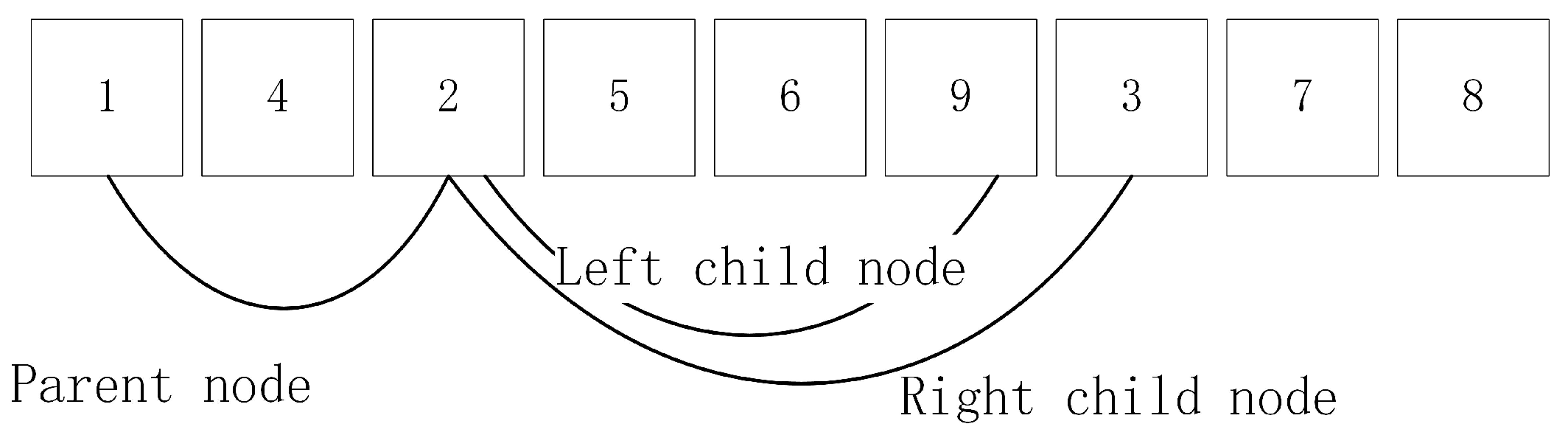
2.1. AMG Method
| Algorithm 1 Pairwise aggregation. |
|
2.2. The AMGPCG Method
3. Comparison of Algorithms
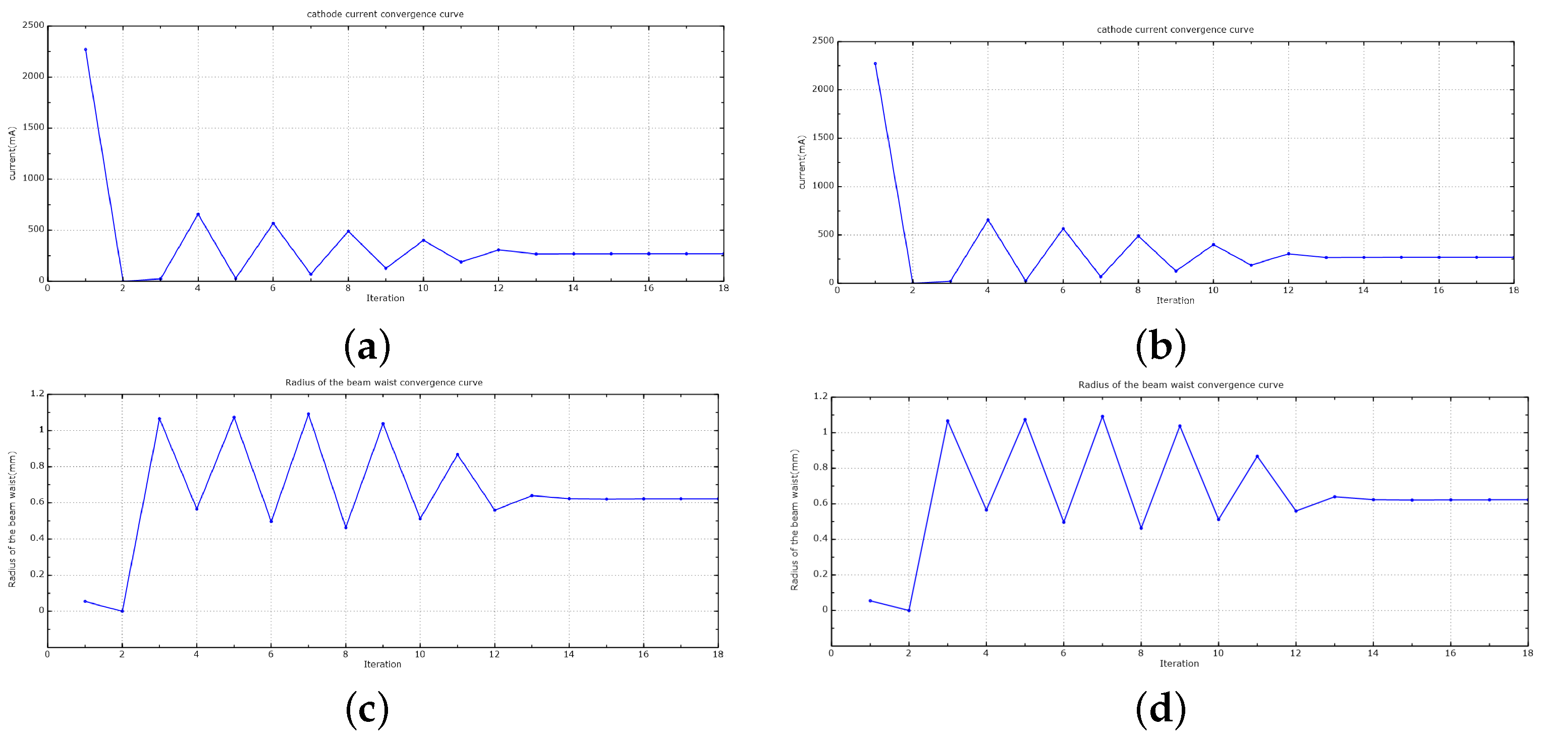
3.1. Verify the Availability of the AMGPCG Solver
3.2. The Information of the Coefficient Matrix
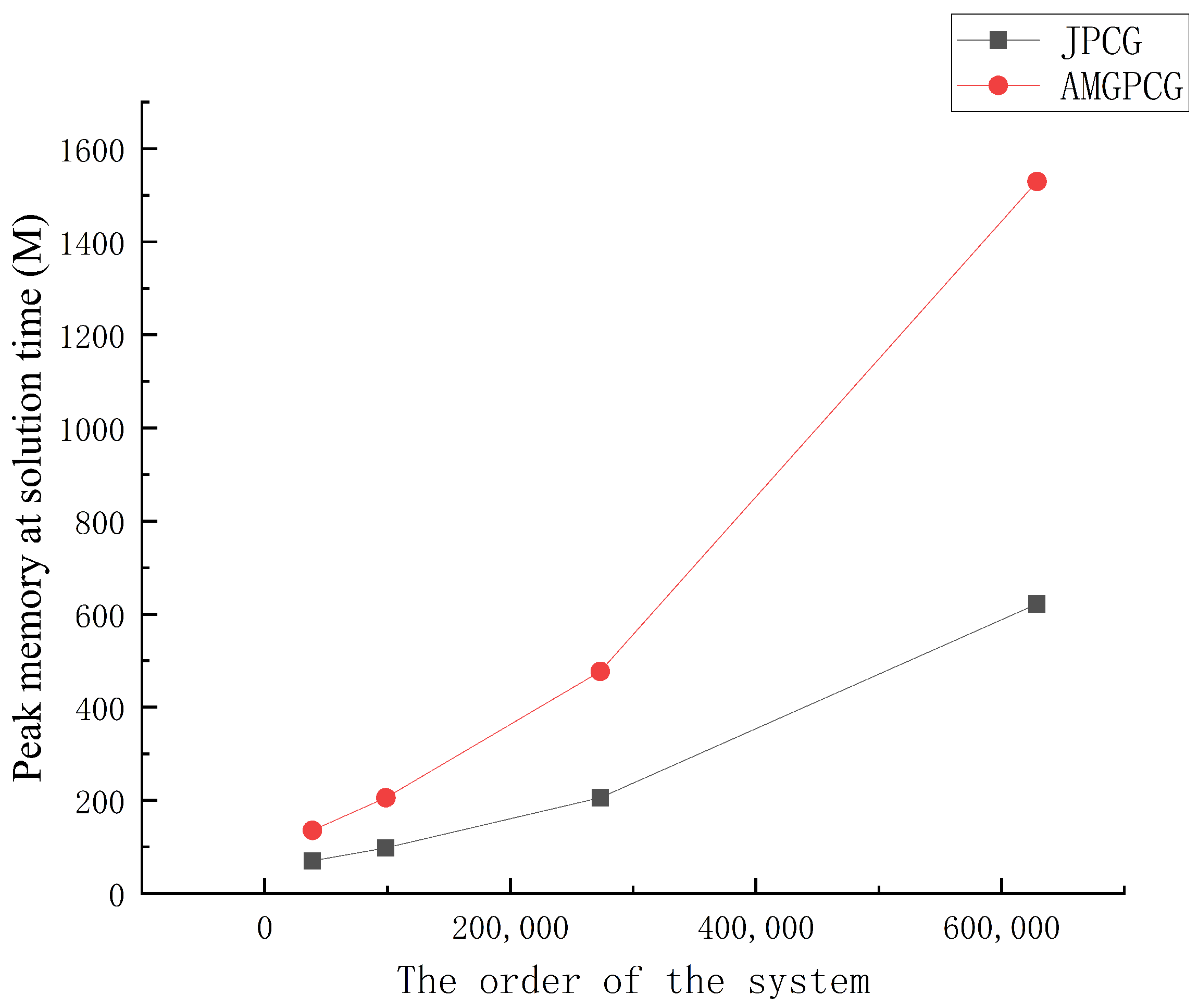
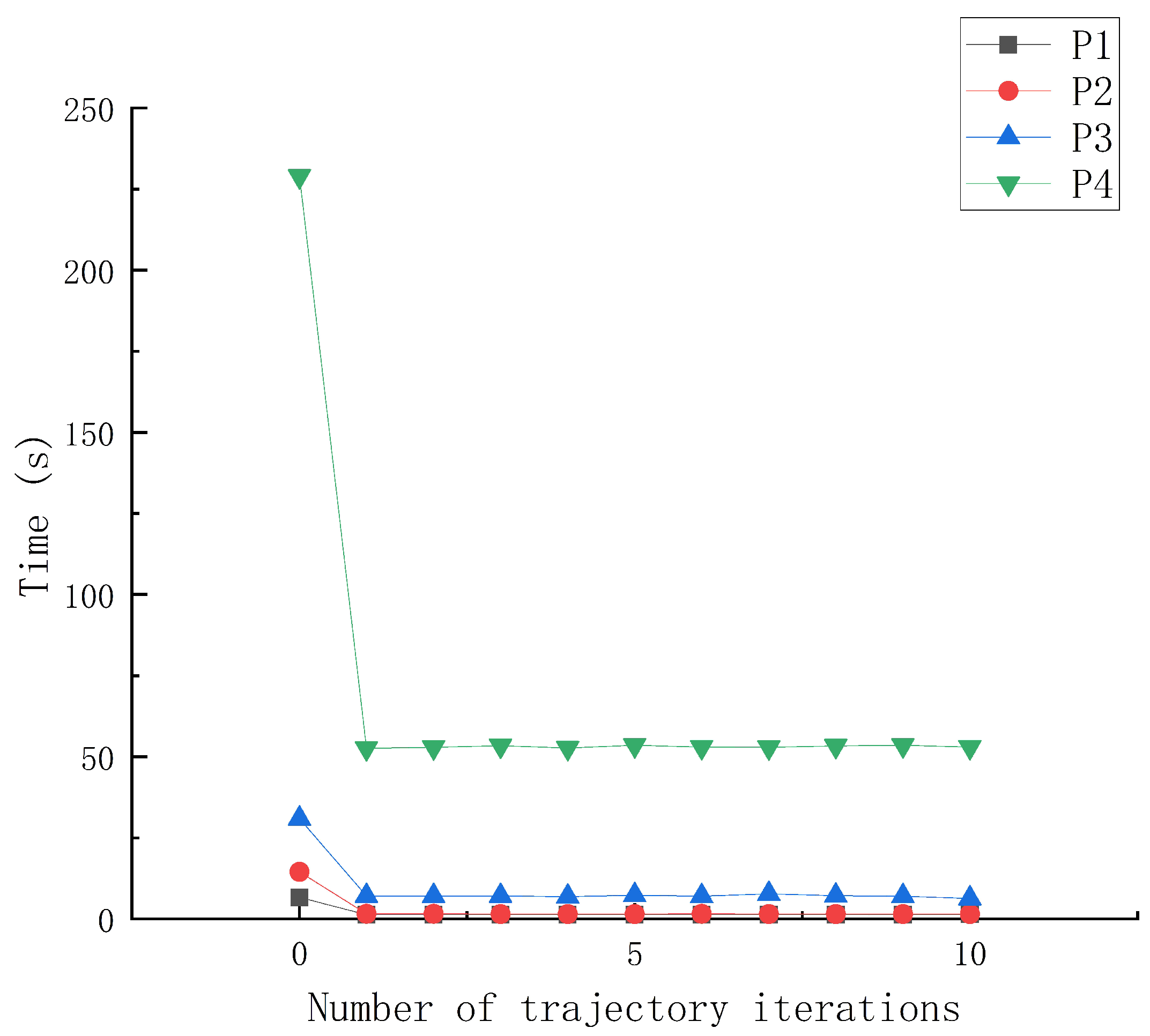
3.3. Comparison of the Calculation Effects
4. Conclusions
Author Contributions
Funding
Institutional Review Board Statement
Informed Consent Statement
Data Availability Statement
Conflicts of Interest
References
- Hu, Q.; Huang, T.; Yang, Z.H.; Li, J.Q.; Jin, X.L.; Zhu, X.F.; Hu, Y.L.; Xu, L.; Li, B. Recent developments on EOS 2-D/3-D electron gun and collector modeling code. IEEE Trans. Electron Devices 2010, 57, 1696–1701. [Google Scholar] [CrossRef]
- Deng, W. Finite element method for the space and time fractional Fokker–Planck equation. SIAM J. Numer. Anal. 2009, 47, 204–226. [Google Scholar] [CrossRef]
- Carson, E.; Higham, N.J. A new analysis of iterative refinement and its application to accurate solution of ill-conditioned sparse linear systems. SIAM J. Sci. Comput. 2017, 39, A2834–A2856. [Google Scholar] [CrossRef]
- Li, J.; Sidford, A.; Tian, K.; Zhang, H. Well-conditioned methods for ill-conditioned systems: Linear regression with semi-random noise. arXiv 2020, arXiv:2008/01722vl. [Google Scholar]
- Steinbach, O.; Yang, H. Comparison of algebraic multigrid methods for an adaptive space–time finite-element discretization of the heat equation in 3D and 4D. Numer. Linear Algebra Appl. 2018, 25, e2143. [Google Scholar] [CrossRef]
- Naumov, M.; Arsaev, M.; Castonguay, P.; Cohen, J.; Demouth, J.; Eaton, J.; Layton, S.; Markovskiy, N.; Reguly, I.; Sakharnykh, N.; et al. AmgX: A library for GPU accelerated algebraic multigrid and preconditioned iterative methods. SIAM J. Sci. Comput. 2015, 37, S602–S626. [Google Scholar] [CrossRef]
- Ganesan, S.; Shah, M. SParSH-AMG: A library for hybrid CPU-GPU algebraic multigrid and preconditioned iterative methods. arXiv 2020, arXiv:2007.00056. [Google Scholar]
- Orozco Aguilar, O.; Arana Ortiz, V.H.; Galindo Nava, A.P. Simulación numérica de yacimientos aplicando los métodos multimalla. Ing. Pet. 2015, 55, 420–433. [Google Scholar]
- Lewis, T.J.; Sastry, S.P.; Kirby, R.M.; Whitaker, R.T. A GPU-based MIS aggregation strategy: Algorithms, comparisons, and applications within AMG. In Proceedings of the 2015 IEEE 22nd International Conference on High Performance Computing (HiPC), Bengaluru, India, 16–19 December 2015; pp. 214–223. [Google Scholar]
- Jnsthvel, T.B.; Gijzen, M.B.V.; Maclachlan, S.; Vuik, C.; Scarpas, A. Comparison of the deflated preconditioned conjugate gradient method and algebraic multigrid for composite materials. Comput. Mech. 2012, 50, 321–333. [Google Scholar] [CrossRef]
- Xu, X.; Zhang, C.S. On the ideal interpolation operator in algebraic multigrid methods. SIAM J. Numer. Anal. 2018, 56, 1693–1710. [Google Scholar] [CrossRef]
- Xu, J.; Zikatanov, L. Algebraic multigrid methods. Acta Numer. 2017, 26, 591–721. [Google Scholar] [CrossRef]
- Xu, X.W. Research on Scalable Parallel Algebraic Multigrid Algorithms. Ph.D. Thesis, Chinese Academy of Engineering Physics, Beijing, China, 2007. [Google Scholar]
- Ruge, J.W.; Stüben, K. Algebraic multigrid. In Multigrid Methods; SIAM: Philadelphia, PA, USA, 1987; pp. 73–130. [Google Scholar]
- Reitzinger, S.; Schöberl, J. An algebraic multigrid method for finite element discretizations with edge elements. Numer. Linear Algebra Appl. 2002, 9, 223–238. [Google Scholar] [CrossRef]
- Manteuffel, T.A.; Olson, L.N.; Schroder, J.B.; Southworth, B.S. A root-node–based algebraic multigrid method. SIAM J. Sci. Comput. 2017, 39, S723–S756. [Google Scholar] [CrossRef]
- Notay, Y. An aggregation-based algebraic multigrid method. Electron. Trans. Numer. Anal. Etna 2010, 37, 123–146. [Google Scholar]
- Webster, R. Stabilisation of AMG solvers for saddle-point stokes problems. Int. J. Numer. Methods Fluids 2016, 81, 640–653. [Google Scholar] [CrossRef]
- Brannick, J.; MacLachlan, S.P.; Schroder, J.B.; Southworth, B.S. The Role of Energy Minimization in Algebraic Multigrid Interpolation. arXiv 2019, arXiv:1902.05157. [Google Scholar]
- Brannick, J.J.; Falgout, R.D. Compatible relaxation and coarsening in algebraic multigrid. SIAM J. Sci. Comput. 2010, 32, 1393–1416. [Google Scholar] [CrossRef]
- Brandt, A.; Brannick, J.; Kahl, K.; Livshits, I. Bootstrap amg. SIAM J. Sci. Comput. 2011, 33, 612–632. [Google Scholar] [CrossRef]
- Feixiao, G. Algebraic Multigrid Solution of Large-Scale Sparse Normal Equation. J. Geomat. Sci. Technol. 2012, 29, 4. [Google Scholar]


| n | 1,220,147 | 96,788 | 1488 | 820 | 694 | 477 | 377 | 201 |
| Problem | n | ||
|---|---|---|---|
| P1 | 47,581 | 0.00023 | 100% |
| P2 | 75,755 | 0.00015 | 100% |
| P3 | 191,714 | 0.00005.9 | 100% |
| P4 | 1,220,147 | 0.0000094 | 100% |
| Problem | Time(s) | Iterations |
|---|---|---|
| Problem: P1 | ||
| V-cycle | 24 | 82 |
| K-cycle t = 0.00 | 29 | 22 |
| K-cycle t = 0.25 | 7 | 23 |
| Problem: P2 | ||
| V-cycle | 60 | 100 |
| K-cycle t = 0.00 | 76 | 22 |
| K-cycle t = 0.25 | 14 | 23 |
| Problem: P3 | ||
| V-cycle | 268 | 178 |
| K-cycle t = 0.00 | 79 | 23 |
| K-cycle t = 0.25 | 30 | 23 |
| Problem: P4 | ||
| V-cycle | 641 | 181 |
| K-cycle t = 0.00 | 519 | 23 |
| K-cycle t = 0.25 | 229 | 23 |
| Problem | Time(s) | Iterations |
|---|---|---|
| Problem: P1 | ||
| AMGPCG | 7 | 23 |
| JPCG | 6 | 1297 |
| CG | 13 | 3500 |
| Gauss–Seidel | 239 | 63,450 |
| Problem: P2 | ||
| AMGPCG | 14 | 23 |
| JPCG | 13 | 1642 |
| CG | 32 | 4423 |
| Gauss–Seidel | 508 | 100,791 |
| Problem: P3 | ||
| AMGPCG | 30 | 23 |
| JPCG | 66 | 2680 |
| CG | 158 | 7258 |
| Gauss–Seidel | 4269 | 242,406 |
| Problem: P4 | ||
| AMGPCG | 229 | 23 |
| JPCG | 1500 | 6771 |
| CG | 3891 | 17,875 |
| Gauss–Seidel | – | >1,000,000 |
| Problem | P1 | P2 | P3 | P4 |
|---|---|---|---|---|
| 80.75% | 89.09% | 77.18% | 77.02% |
Publisher’s Note: MDPI stays neutral with regard to jurisdictional claims in published maps and institutional affiliations. |
© 2022 by the authors. Licensee MDPI, Basel, Switzerland. This article is an open access article distributed under the terms and conditions of the Creative Commons Attribution (CC BY) license (https://creativecommons.org/licenses/by/4.0/).
Share and Cite
Wang, Z.; Hu, Q.; Zhu, X.-F.; Li, B.; Hu, Y.-L.; Huang, T.; Yang, Z.-H.; Li, L. Research of the Algebraic Multigrid Method for Electron Optical Simulator. Entropy 2022, 24, 1133. https://doi.org/10.3390/e24081133
Wang Z, Hu Q, Zhu X-F, Li B, Hu Y-L, Huang T, Yang Z-H, Li L. Research of the Algebraic Multigrid Method for Electron Optical Simulator. Entropy. 2022; 24(8):1133. https://doi.org/10.3390/e24081133
Chicago/Turabian StyleWang, Zhi, Quan Hu, Xiao-Fang Zhu, Bin Li, Yu-Lu Hu, Tao Huang, Zhong-Hai Yang, and Liang Li. 2022. "Research of the Algebraic Multigrid Method for Electron Optical Simulator" Entropy 24, no. 8: 1133. https://doi.org/10.3390/e24081133
APA StyleWang, Z., Hu, Q., Zhu, X.-F., Li, B., Hu, Y.-L., Huang, T., Yang, Z.-H., & Li, L. (2022). Research of the Algebraic Multigrid Method for Electron Optical Simulator. Entropy, 24(8), 1133. https://doi.org/10.3390/e24081133