
Multiscale Methods for Signal Selection in Single-Cell Data

 , , ,
, , ,
Abstract
:1. Introduction
2. Materials and Methods
2.1. Preliminaries
2.2. Eigenscores
2.2.1. The 0th Eigenscore
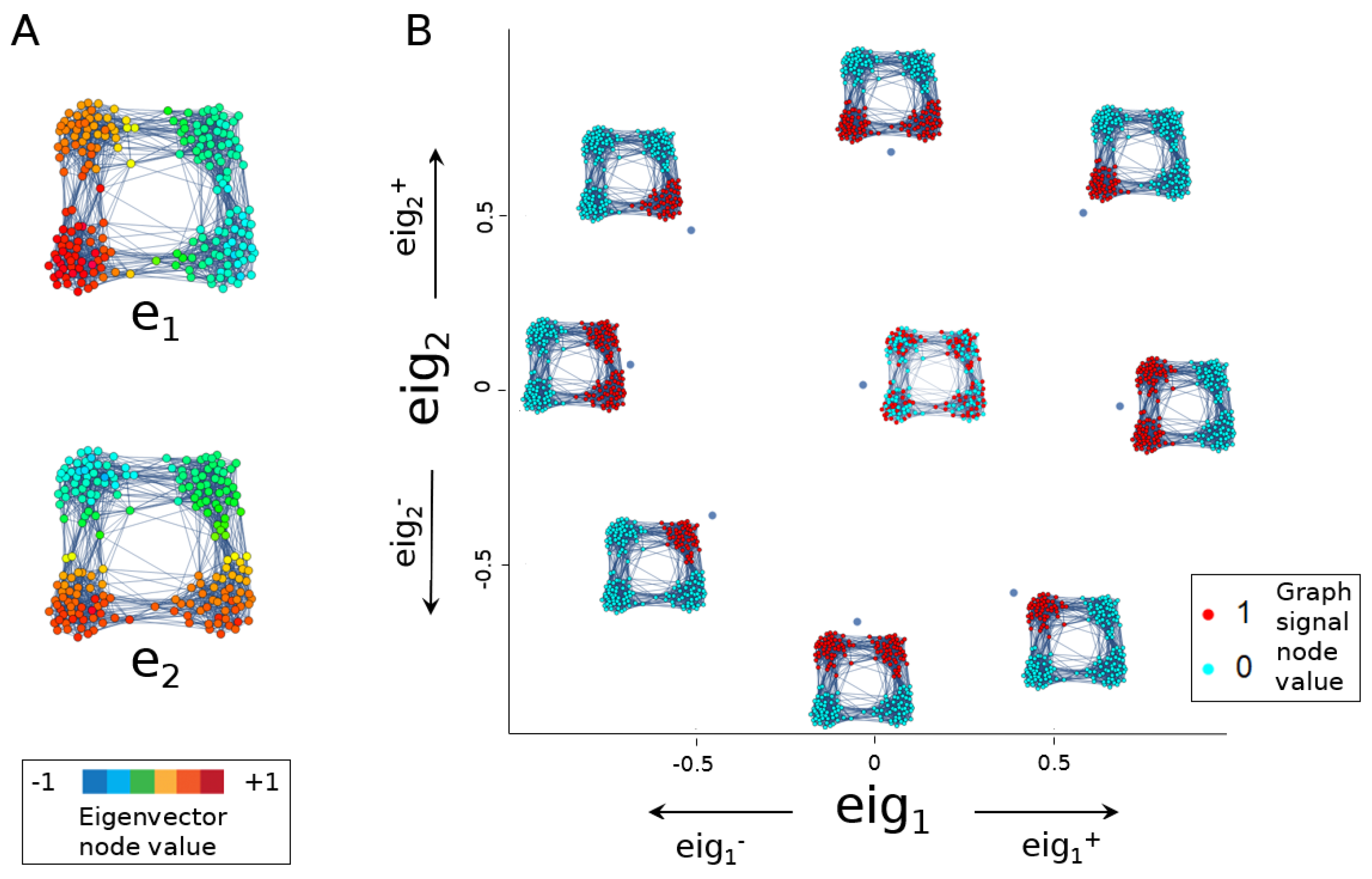
2.2.2. Eigenscores to Visualise Graph Signals
2.3. Multiscale Laplacian Score
2.3.1. Random Walks on Graphs
2.3.2. Community Detection
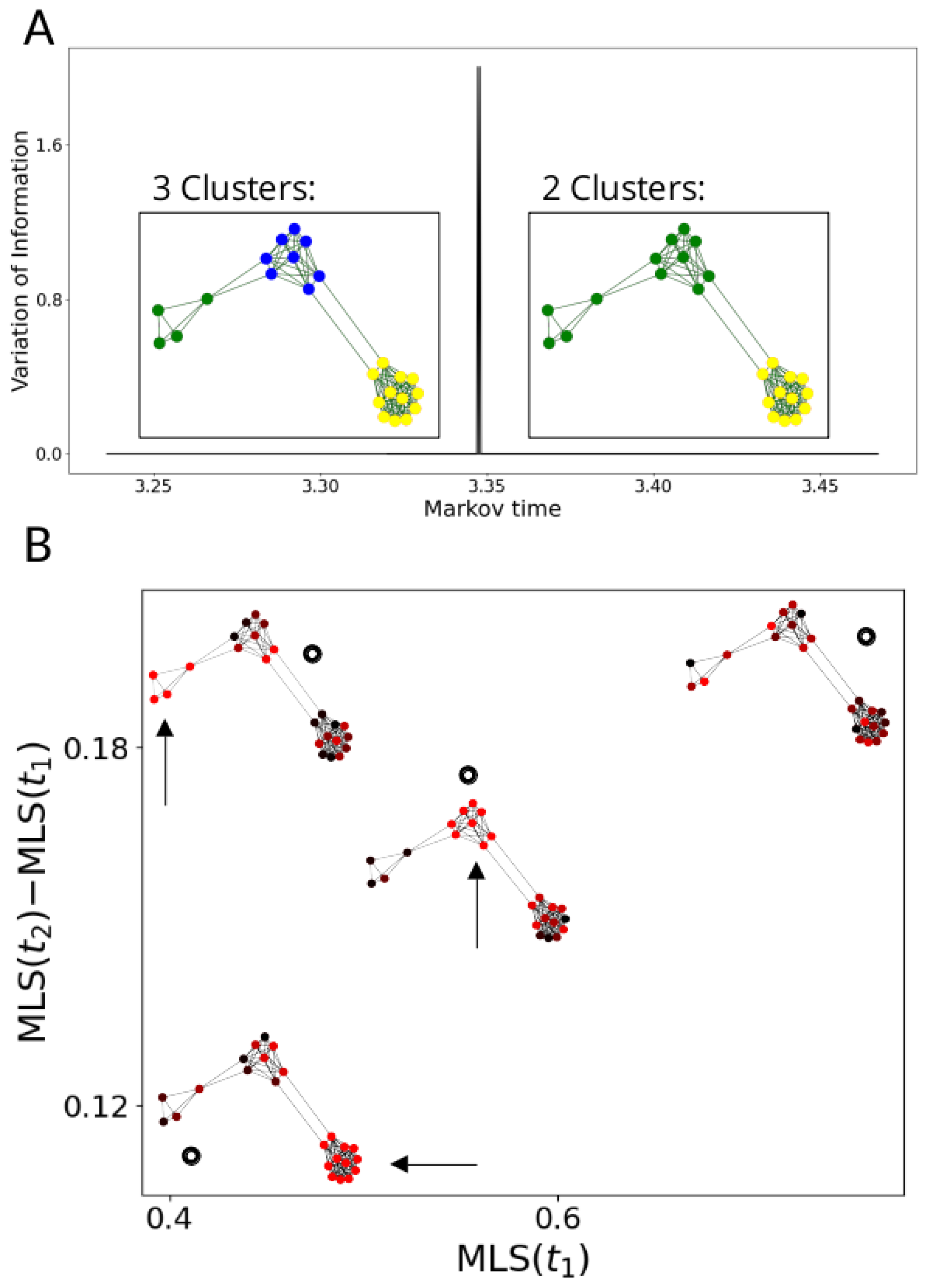
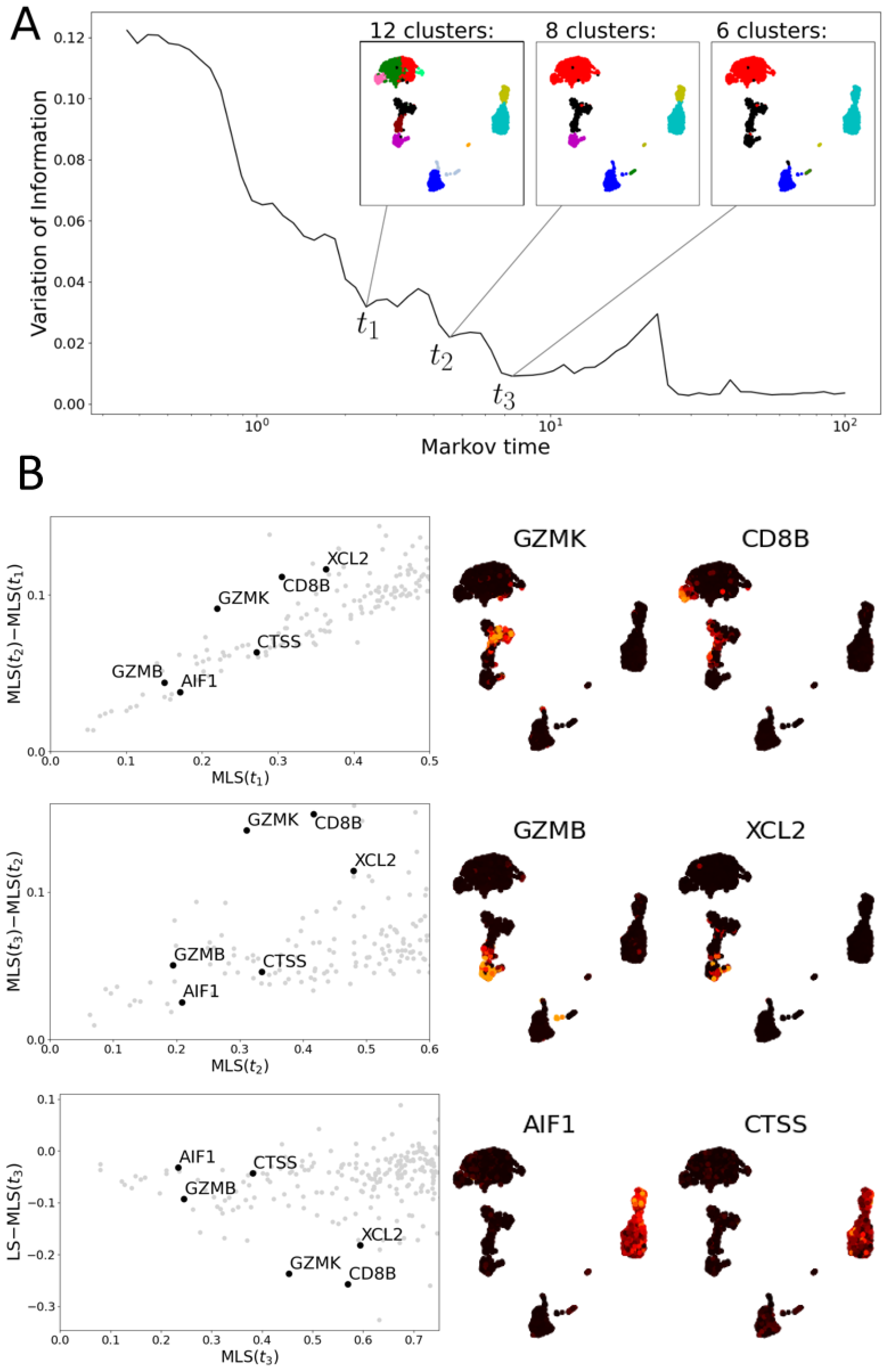
2.3.3. Signal Scores at Multiple Resolutions
2.3.4. MLS Analysis Pipeline
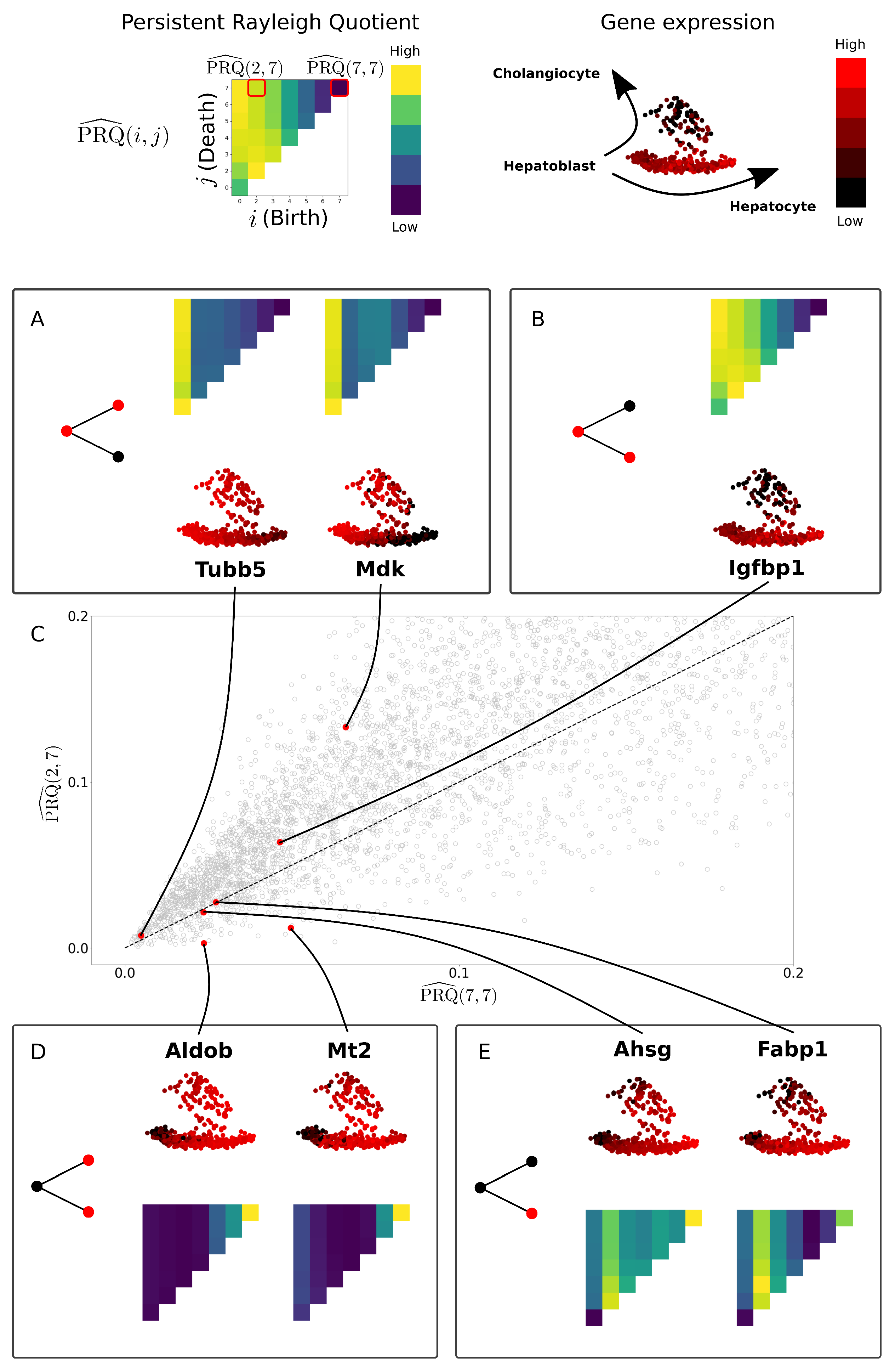
2.4. Persistent Rayleigh Quotient
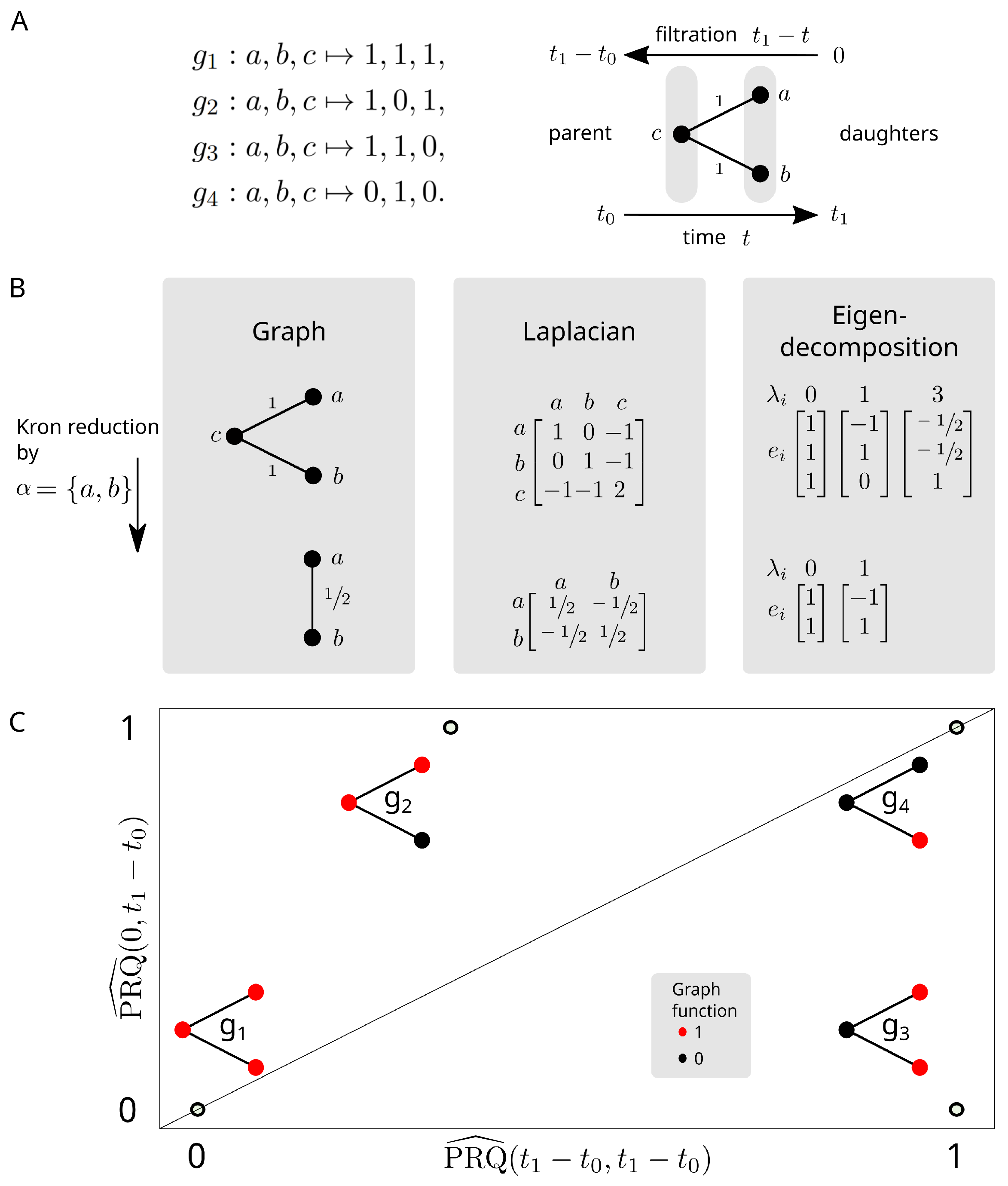
2.4.1. Persistent Laplacian
- 1.
- is well-defined as is invertible.
- 2.
- is symmetric.
- 3.
- , where is the column vector of ones.
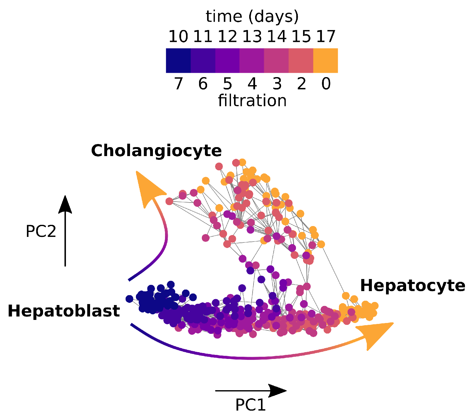
2.4.2. Application to Cell Bifurcation
2.5. Data Sets
2.5.1. Preprocessing of PBMC and T Cell Data Sets
2.5.2. Preprocessing of Mouse Foetal Liver Cell Data Set
2.5.3. Previous Results on PBMC Data
2.5.4. Previous Results on T Cell Data
2.5.5. Previous Results on Mouse Foetal Liver Cell Data Set
2.6. Code Availability
3. Results
3.1. Eigenscores
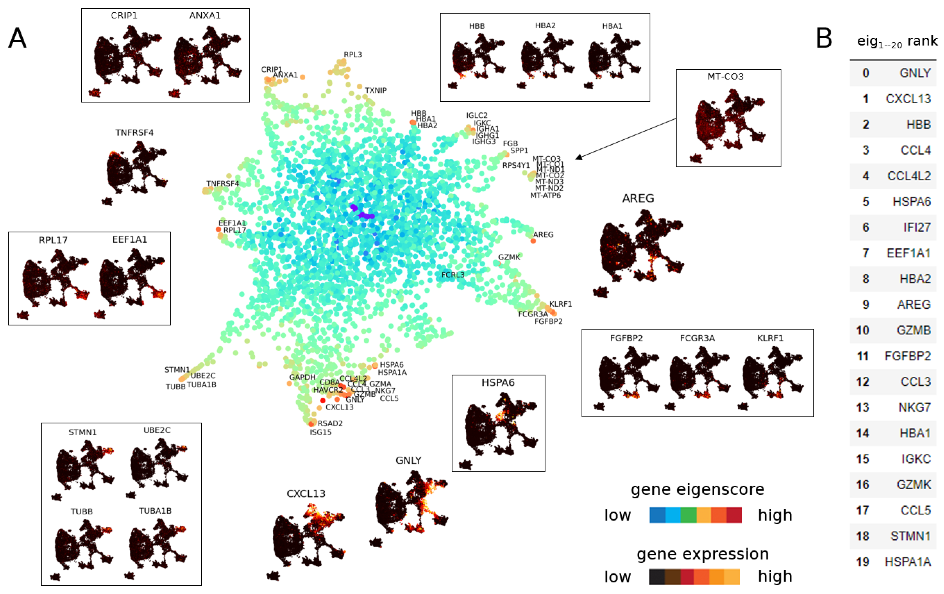
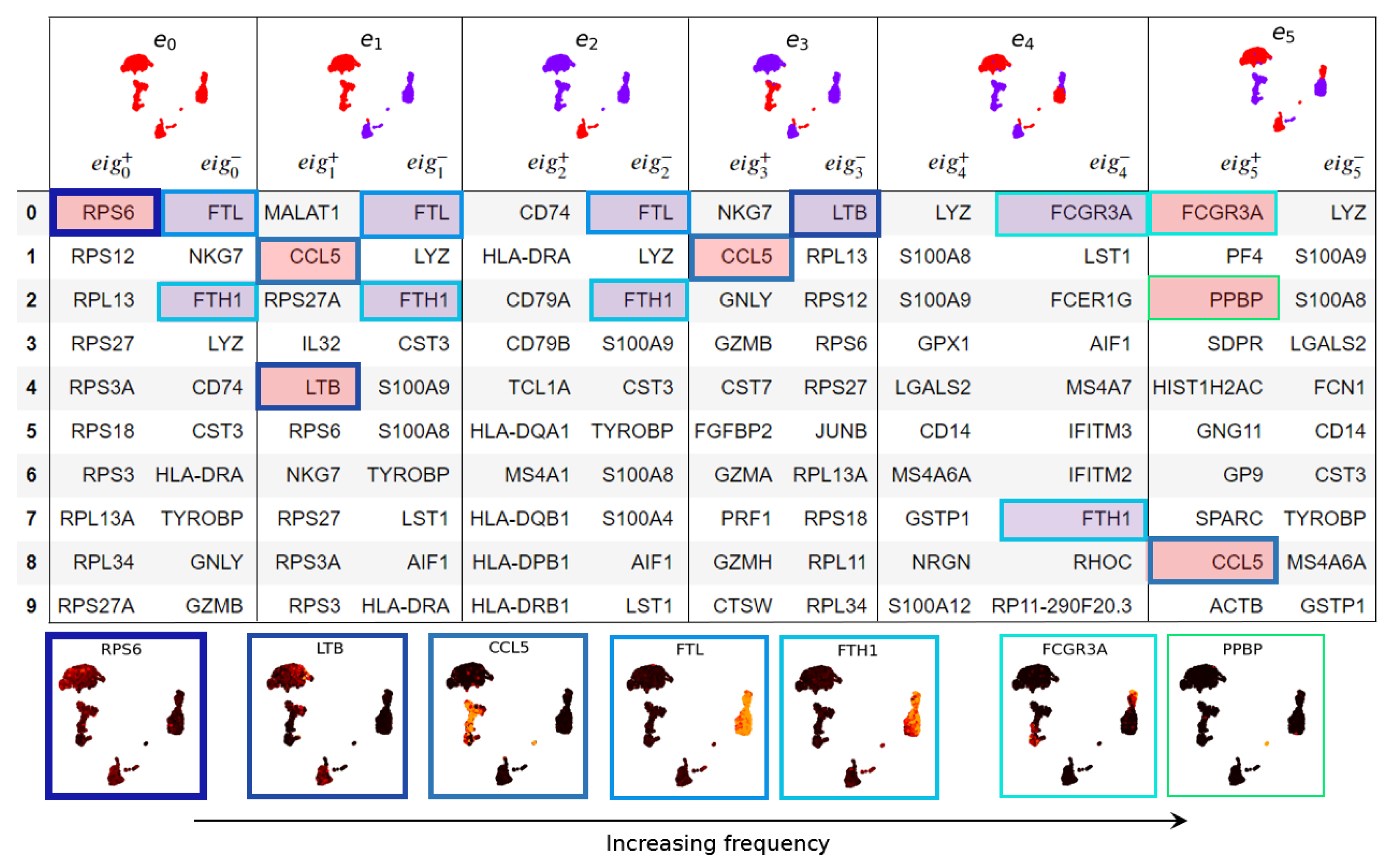
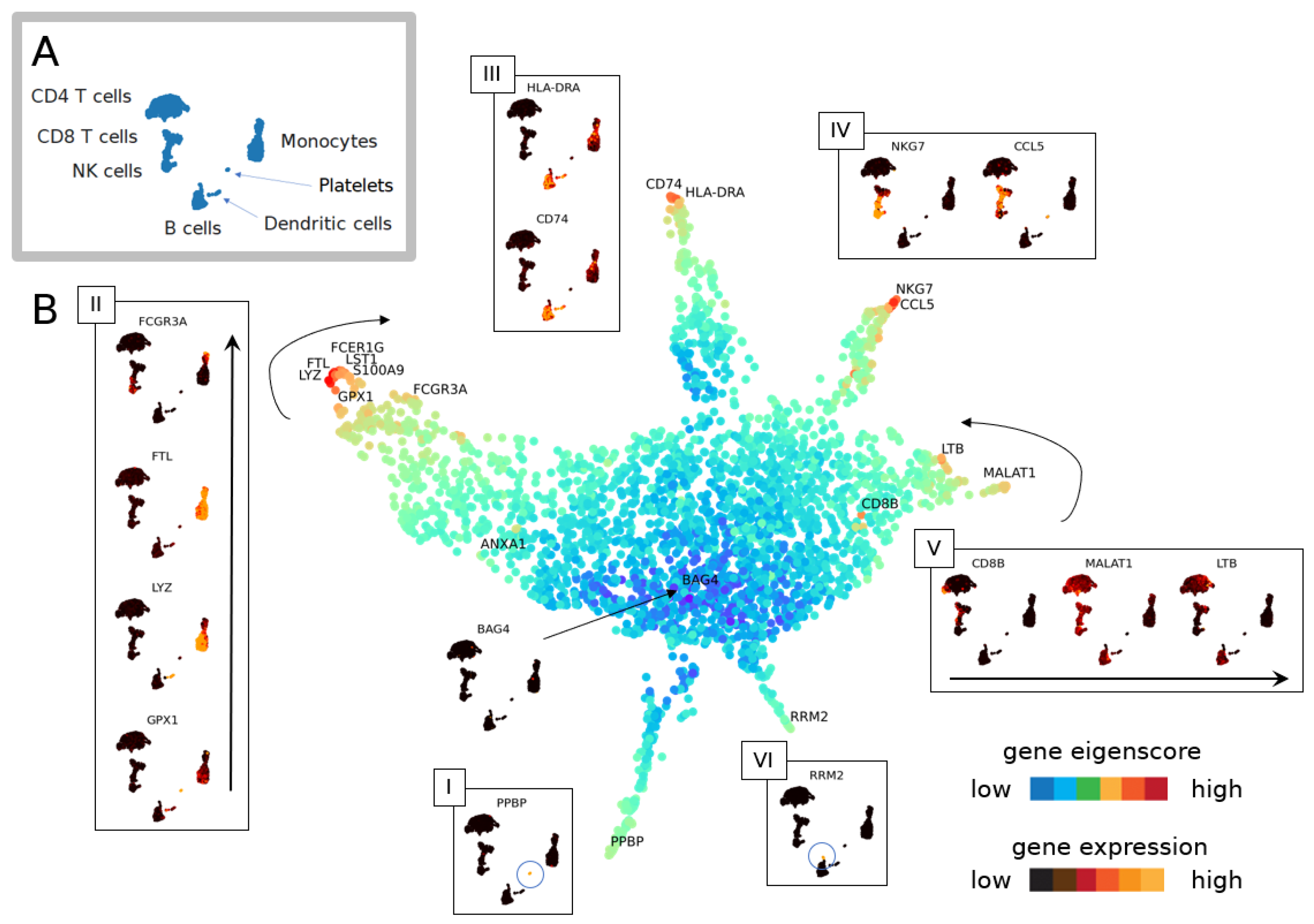
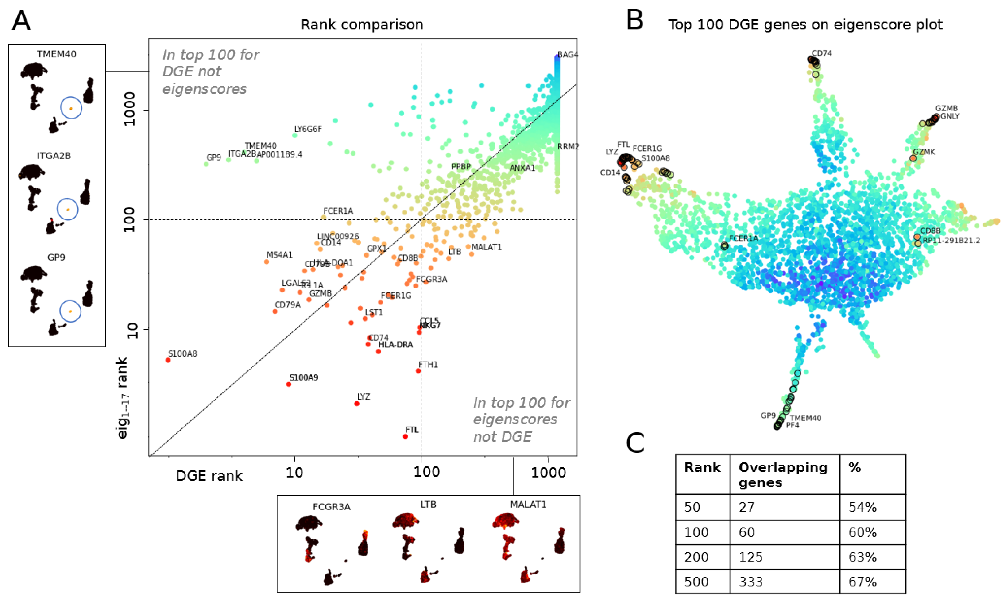
3.1.1. The Geometry of PBMC Genes via Eigenscores
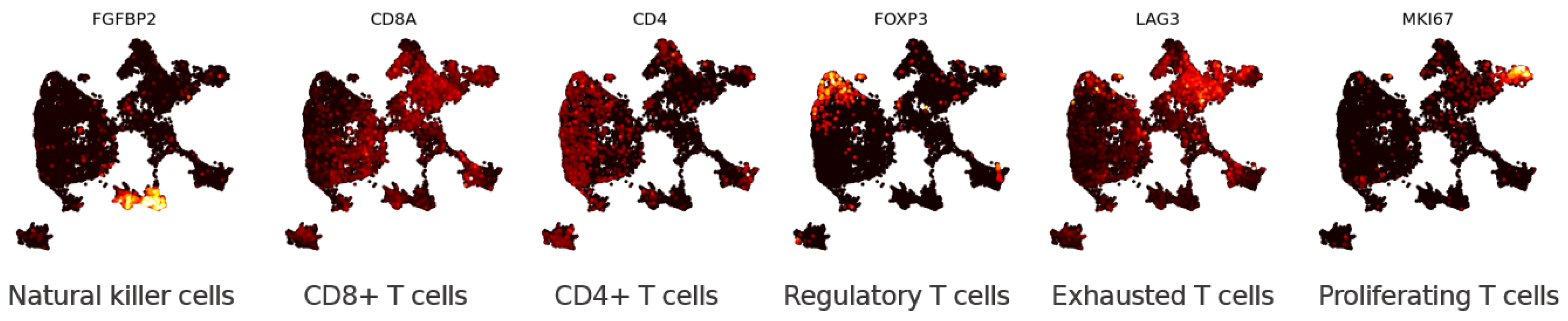
3.1.2. Eigenscores for Analysing Data with Continuous Structure: T Cells
3.2. Multiscale Laplacian Score
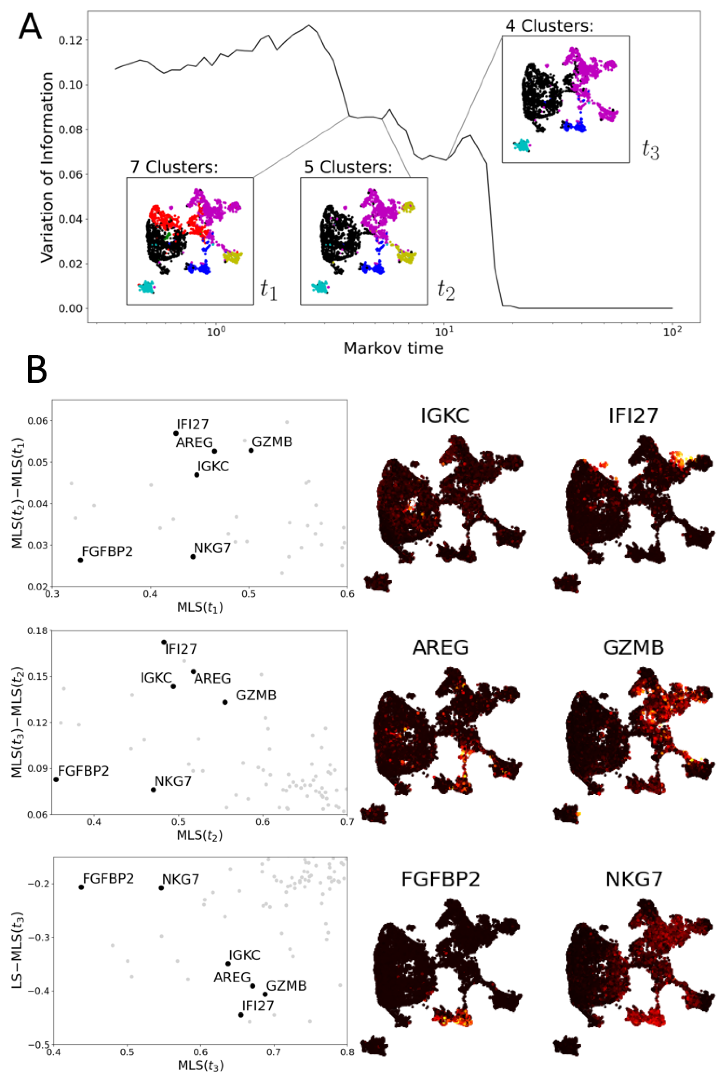
3.2.1. Multiscale Laplacian Score of PBMC Data
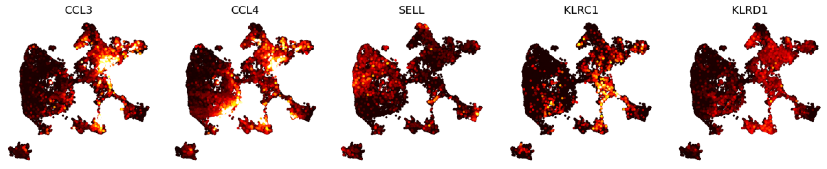
3.2.2. Multiscale Laplacian Score of T Cell Data
3.3. Persistent Rayleigh Quotient
4. Conclusions
Author Contributions
Funding
Institutional Review Board Statement
Informed Consent Statement
Data Availability Statement
Acknowledgments
Conflicts of Interest
Appendix A


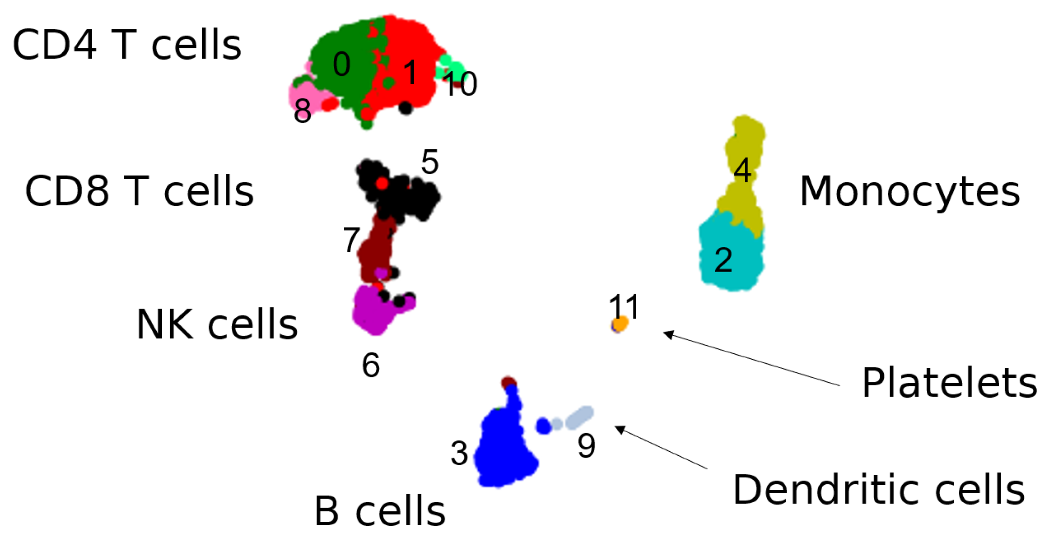
| 0 | 1 | 2 | 3 | 4 | 5 | 6 | 7 | 8 | 9 | 10 | 11 | |
|---|---|---|---|---|---|---|---|---|---|---|---|---|
| 0 | RPS27 | LTB | S100A8 | CD79A | IFITM3 | GZMK | GZMB | GZMH | CD8B | FCER1A | IFIT1 | GP9 |
| 1 | RPL32 | IL32 | LGALS2 | MS4A1 | RP11-290F20.3 | CCL5 | FGFBP2 | CST7 | RP11-291B21.2 | ENHO | IFIT3 | ITGA2B |
| 2 | RPS6 | IL7R | S100A9 | TCL1A | LST1 | NKG7 | SPON2 | NKG7 | CD8A | CLEC10A | RTP4 | TMEM40 |
| 3 | RPS12 | CD3D | CD14 | CD79B | AIF1 | LYAR | GNLY | CCL5 | S100B | SERPINF1 | SPATS2L | AP001189.4 |
| 4 | RPL31 | AQP3 | FCN1 | HLA-DQA1 | MS4A7 | GZMA | PRF1 | GZMA | CARS | CD1C | DDX58 | LY6G6F |
| 5 | RPS14 | LDHB | TYROBP | LINC00926 | IFI30 | IL32 | XCL2 | FGFBP2 | RPS12 | CACNA2D3 | RSAD2 | sep-05 |
| 6 | RPS25 | CD2 | MS4A6A | VPREB3 | CD68 | CD8A | AKR1C3 | CD8A | RPL13 | HLA-DQB2 | MX1 | HGD |
| 7 | LDHB | CD40LG | LYZ | HLA-DQB1 | FCER1G | CTSW | CLIC3 | GZMB | RPS6 | HLA-DQA2 | ISG15 | PTCRA |
| 8 | RPS3A | TPT1 | GPX1 | CD74 | CFD | CST7 | KLRD1 | CTSW | CCR7 | HLA-DQA1 | IFI6 | TREML1 |
| 9 | RPL30 | CD3E | CST3 | HLA-DRA | SERPINA1 | HOPX | CST7 | CCL4 | RPL32 | NDRG2 | HERC5 | ITGB3 |

References
- Hao, Y.; Hao, S.; Andersen-Nissen, E.; Mauck, W.M., III; Zheng, S.; Butler, A.; Lee, M.J.; Wilk, A.J.; Darby, C.; Zagar, M.; et al. Integrated analysis of multimodal single-cell data. Cell 2021, 184, 3573–3587. [Google Scholar] [CrossRef] [PubMed]
- Wolf, F.A.; Angerer, P.; Theis, F.J. SCANPY: Large-scale single-cell gene expression data analysis. Genome Biol. 2018, 19, 1–5. [Google Scholar] [CrossRef]
- McInnes, L.; Healy, J.; Saul, N.; Großberger, L. UMAP: Uniform Manifold Approximation and Projection. J. Open Source Softw. 2018, 3, 861. [Google Scholar] [CrossRef]
- Becht, E.; McInnes, L.; Healy, J.; Dutertre, C.A.; Kwok, I.W.; Ng, L.G.; Ginhoux, F.; Newell, E.W. Dimensionality reduction for visualizing single-cell data using UMAP. Nat. Biotechnol. 2019, 37, 38–44. [Google Scholar] [CrossRef] [PubMed]
- Jeitziner, R.; Carrière, M.; Rougemont, J.; Oudot, S.; Hess, K.; Brisken, C. Two-tier mapper: A user-independent clustering method for global gene expression analysis based on topology. arXiv 2017, arXiv:1801.01841. [Google Scholar]
- Rizvi, A.H.; Camara, P.G.; Kandror, E.K.; Roberts, T.J.; Schieren, I.; Maniatis, T.; Rabadan, R. Single-Cell Topological RNA-Seq Analysis Reveals Insights into Cellular Differentiation and Development. Nat. Biotechnol. 2017, 35, 551–560. [Google Scholar] [CrossRef]
- Kuchroo, M.; DiStasio, M.; Calapkulu, E.; Ige, M.; Zhang, L.; Sheth, A.H.; Menon, M.; Xing, Y.; Gigante, S.; Huang, J.; et al. Topological Analysis of Single-Cell Data Reveals Shared Glial Landscape of Macular Degeneration and Neurodegenerative Diseases. bioRxiv 2012. [Google Scholar] [CrossRef]
- Vandaele, R.; Rieck, B.; Saeys, Y.; De Bie, T. Stable Topological Signatures for Metric Trees through Graph Approximations. Pattern Recog. Lett. 2021, 147, 85–92. [Google Scholar] [CrossRef]
- Ortega, A.; Frossard, P.; Kovačević, J.; Moura, J.M.; Vandergheynst, P. Graph signal processing: Overview, challenges, and applications. Proc. IEEE 2018, 106, 808–828. [Google Scholar] [CrossRef]
- Chung, F.R. Spectral Graph Theory; Number 92; American Mathematical Soc.: Providence, RI, USA, 1997. [Google Scholar]
- Robinson, M. Topological Signal Processing; Springer: Berlin/Heidelberg, Germany, 2014; Volume 8. [Google Scholar]
- Schaub, M.T.; Zhu, Y.; Seby, J.B.; Roddenberry, T.M.; Segarra, S. Signal processing on higher-order networks: Livin’on the edge... and beyond. Signal Process. 2021, 187, 108149. [Google Scholar] [CrossRef]
- Barbarossa, S.; Sardellitti, S. Topological signal processing over simplicial complexes. IEEE Trans. Signal Process. 2020, 68, 2992–3007. [Google Scholar] [CrossRef]
- He, X.; Cai, D.; Niyogi, P. Laplacian score for feature selection. Adv. Neural Inf. Process. Syst. 2005, 18, 1–8. [Google Scholar]
- Govek, K.W.; Yamajala, V.S.; Camara, P.G. Clustering-Independent Analysis of Genomic Data Using Spectral Simplicial Theory. PLoS Comput. Biol. 2019, 15, e1007509. [Google Scholar] [CrossRef]
- Delvenne, J.C.; Schaub, M.T.; Yaliraki, S.N.; Barahona, M. The stability of a graph partition: A dynamics-based framework for community detection. In Dynamics On and Of Complex Networks, Volume 2; Springer: Berlin/Heidelberg, Germany, 2013; pp. 221–242. [Google Scholar]
- Schaub, M.T.; Delvenne, J.C.; Yaliraki, S.N.; Barahona, M. Markov Dynamics as a Zooming Lens for MultiscaleCommunity Detection: Non Clique-Like Communitiesand the Field-of-View Limit. PLoS ONE 2012, 7, e32210. [Google Scholar] [CrossRef]
- Dorfler, F.; Bullo, F. Kron Reduction of Graphs With Applications to Electrical Networks. IEEE Trans. Circ. Syst. I Regul. Pap. 2013, 60, 150–163. [Google Scholar] [CrossRef]
- Wang, R.; Nguyen, D.D.; Wei, G.W. Persistent spectral graph. Int. J. Numer. Methods Biomed. Eng. 2020, 36, e3376. [Google Scholar] [CrossRef]
- Mémoli, F.; Wan, Z.; Wang, Y. Persistent Laplacians: Properties, Algorithms and Implications. arXiv 2021, arXiv:2012.02808. [Google Scholar] [CrossRef]
- Belkin, M.; Niyogi, P. Laplacian eigenmaps for dimensionality reduction and data representation. Neural Comput. 2003, 15, 1373–1396. [Google Scholar] [CrossRef]
- Calvetti, D.; Reichel, L.; Sorensen, D.C. An implicitly restarted Lanczos method for large symmetric eigenvalue problems. Electron. Trans. Numer. Anal. 1994, 2, 21. [Google Scholar]
- Delvenne, J.C.; Yaliraki, S.N.; Barahona, M. Stability of graph communities across time scales. Proc. Natl. Acad. Sci. USA 2010, 107, 12755–12760. [Google Scholar] [CrossRef]
- Lambiotte, R.; Delvenne, J.C.; Barahona, M. Random walks, Markov processes and the multiscale modular organization of complex networks. IEEE Trans. Netw. Sci. Eng. 2014, 1, 76–90. [Google Scholar] [CrossRef]
- Masuda, N.; Porter, M.A.; Lambiotte, R. Random walks and diffusion on networks. Phys. Rep. 2017, 716, 1–58. [Google Scholar] [CrossRef]
- Porter, M.A.; Onnela, J.P.; Mucha, P.J. Communities in networks. Not. AMS 2009, 56, 1082–1097. [Google Scholar]
- Blondel, V.D.; Guillaume, J.L.; Lambiotte, R.; Lefebvre, E. Fast unfolding of communities in large networks. J. Stat. Mech. Theory Exp. 2008, 2008, P10008. [Google Scholar] [CrossRef]
- Bacik, K.A.; Schaub, M.T.; Beguerisse-Díaz, M.; Billeh, Y.N.; Barahona, M. Flow-based network analysis of the Caenorhabditis elegans connectome. PLoS Comput. Biol. 2016, 12, e1005055. [Google Scholar] [CrossRef]
- Beguerisse-Diaz, M.; Vangelov, B.; Barahona, M. Finding role communities in directed networks using Role-Based Similarity, Markov Stability and the Relaxed Minimum Spanning Tree. In Proceedings of the 2013 IEEE Global Conference on Signal and Information Processing, Austin, TX, USA, 3–5 December 2013. [Google Scholar]
- Liu, Z.; Barahona, M. Graph-based data clustering via multiscale community detection. Appl. Netw. Sci. 2020, 5, 1–20. [Google Scholar] [CrossRef]
- Meilă, M. Comparing clusterings—An information based distance. J. Multivar. Anal. 2007, 98, 873–895. [Google Scholar] [CrossRef]
- Barahona, M. The Stability of a Graph Partition. Available online: https://www.ma.imperial.ac.uk/~mpbara/Partition_Stability/ (accessed on 23 May 2022).
- Ghrist, R. Barcodes: The persistent topology of data. Bull. Am. Math. Soc. 2008, 45, 61–75. [Google Scholar] [CrossRef]
- Genomics 1. 10X Peripheral Blood Mononuclear Cells (PBMC) Data. 1 June 2022. Available online: https://cf.10xgenomics.com/samples/cell/pbmc3k/pbmc3k_filtered_gene_bc_matrices.tar.gz (accessed on 1 June 2022).
- Satija Lab, N. Seurat Guided Clustering Tutorial. Available online: https://satijalab.org/seurat/articles/pbmc3k_tutorial.html (accessed on 23 May 2022).
- Hafemeister, C.; Satija, R. Using Sctransform in Seurat. Available online: https://satijalab.org/seurat/articles/sctransform_vignette.html (accessed on 23 May 2022).
- Wolf, A.; Ramirez, F.; Rybakov, S. Scanpy Tutorials Preprocessing and Clustering 3k PBMCs. Available online: https://scanpy-tutorials.readthedocs.io/en/latest/pbmc3k.html (accessed on 2 August 2022).
- Lambrechts, D.; Wauters, E.; Boeckx, B.; Aibar, S.; Nittner, D.; Burton, O.; Bassez, A.; Decaluwé, H.; Pircher, A.; Van den Eynde, K.; et al. Phenotype molding of stromal cells in the lung tumor microenvironment. Nat. Med. 2018, 24, 1277–1289. [Google Scholar] [CrossRef]
- Yang, L.; Wang, W.H.; Qiu, W.L.; Guo, Z.; Bi, E.; Xu, C.R. A Single-Cell Transcriptomic Analysis Reveals Precise Pathways and Regulatory Mechanisms Underlying Hepatoblast Differentiation. Hepatology 2017, 66, 1387–1401. [Google Scholar] [CrossRef]
- Hafemeister, C.; Satija, R. Normalization and variance stabilization of single-cell RNA-seq data using regularized negative binomial regression. Genome Biol. 2019, 20, 1–15. [Google Scholar] [CrossRef] [PubMed]
- Satija Lab, NYU. Differential Expression Testing. Available online: https://satijalab.org/seurat/articles/de_vignette.html (accessed on 23 July 2022).
- Mu, T.; Xu, L.; Zhong, Y.; Liu, X.; Zhao, Z.; Huang, C.; Lan, X.; Lufei, C.; Zhou, Y.; Su, Y.; et al. Embryonic Liver Developmental Trajectory Revealed by Single-Cell RNA Sequencing in the Foxa2eGFP Mouse. Commun. Biol. 2020, 3, 1–12. [Google Scholar] [CrossRef] [PubMed]
- Alvarez, M.; Rahmani, E.; Jew, B.; Garske, K.M.; Miao, Z.; Benhammou, J.N.; Ye, C.J.; Pisegna, J.R.; Pietiläinen, K.H.; Halperin, E.; et al. Enhancing droplet-based single-nucleus RNA-seq resolution using the semi-supervised machine learning classifier DIEM. Sci. Rep. 2020, 10, 11019. [Google Scholar] [CrossRef] [PubMed]
- Rindler, K.; Bauer, W.M.; Jonak, C.; Wielscher, M.; Shaw, L.E.; Rojahn, T.B.; Thaler, F.M.; Porkert, S.; Simonitsch-Klupp, I.; Weninger, W.; et al. Single-cell RNA sequencing reveals tissue compartment-specific plasticity of mycosis fungoides tumor cells. Front. Immunol. 2021, 12, 666935. [Google Scholar] [CrossRef] [PubMed]
- Sookoian, S.; Flichman, D.; Garaycoechea, M.E.; San Martino, J.; Castaño, G.O.; Pirola, C.J. Metastasis-associated lung adenocarcinoma transcript 1 as a common molecular driver in the pathogenesis of nonalcoholic steatohepatitis and chronic immune-mediated liver damage. Hepatol. Commun. 2018, 2, 654–665. [Google Scholar] [CrossRef] [PubMed]
- Cohen, L.A.; Gutierrez, L.; Weiss, A.; Leichtmann-Bardoogo, Y.; Zhang, D.l.; Crooks, D.R.; Sougrat, R.; Morgenstern, A.; Galy, B.; Hentze, M.W.; et al. Serum ferritin is derived primarily from macrophages through a nonclassical secretory pathway. Blood J. Am. Soc. Hematol. 2010, 116, 1574–1584. [Google Scholar] [CrossRef] [PubMed]
- Theurl, I.; Mattle, V.; Seifert, M.; Mariani, M.; Marth, C.; Weiss, G. Dysregulated monocyte iron homeostasis and erythropoietin formation in patients with anemia of chronic disease. Blood 2006, 107, 4142–4148. [Google Scholar] [CrossRef]
- Zarjou, A.; Black, L.M.; McCullough, K.R.; Hull, T.D.; Esman, S.K.; Boddu, R.; Varambally, S.; Chandrashekar, D.S.; Feng, W.; Arosio, P.; et al. Ferritin light chain confers protection against sepsis-induced inflammation and organ injury. Front. Immunol. 2019, 10, 131. [Google Scholar] [CrossRef]
- Pizzolato, G.; Kaminski, H.; Tosolini, M.; Franchini, D.M.; Pont, F.; Martins, F.; Valle, C.; Labourdette, D.; Cadot, S.; Quillet-Mary, A.; et al. Single-cell RNA sequencing unveils the shared and the distinct cytotoxic hallmarks of human TCRVδ1 and TCRVδ2 γδ T lymphocytes. Proc. Natl. Acad. Sci. USA 2019, 116, 11906–11915. [Google Scholar] [CrossRef]
- Geng, Z.; Tao, Y.; Zheng, F.; Wu, L.; Wang, Y.; Wang, Y.; Sun, Y.; Fu, S.; Wang, W.; Xie, C.; et al. Altered monocyte subsets in Kawasaki disease revealed by single-cell RNA-sequencing. J. Inflamm. Res. 2021, 14, 885. [Google Scholar] [CrossRef]
- Cormican, S.; Griffin, M.D. Human monocyte subset distinctions and function: Insights from gene expression analysis. Front. Immunol. 2020, 11, 1070. [Google Scholar] [CrossRef] [PubMed]
- Victor, A.R.; Weigel, C.; Scoville, S.D.; Chan, W.K.; Chatman, K.; Nemer, M.M.; Mao, C.; Young, K.A.; Zhang, J.; Yu, J.; et al. Epigenetic and posttranscriptional regulation of CD16 expression during human NK cell development. J. Immunol. 2018, 200, 565–572. [Google Scholar] [CrossRef] [PubMed]
- Crinier, A.; Dumas, P.Y.; Escalière, B.; Piperoglou, C.; Gil, L.; Villacreces, A.; Vély, F.; Ivanovic, Z.; Milpied, P.; Narni-Mancinelli, É.; et al. Single-cell profiling reveals the trajectories of natural killer cell differentiation in bone marrow and a stress signature induced by acute myeloid leukemia. Cell. Mol. Immunol. 2021, 18, 1290–1304. [Google Scholar] [CrossRef]
- Stegle, O.; Teichmann, S.A.; Marioni, J.C. Computational and analytical challenges in single-cell transcriptomics. Nat. Rev. Genet. 2015, 16, 133–145. [Google Scholar] [CrossRef] [PubMed]
- Lee, R.D.; Munro, S.A.; Knutson, T.P.; LaRue, R.S.; Heltemes-Harris, L.M.; Farrar, M.A. Single-cell analysis identifies dynamic gene expression networks that govern B cell development and transformation. Nat. Commun. 2021, 12, 1–16. [Google Scholar] [CrossRef] [PubMed]
- Ullah, H.; Sajid, M.; Yan, K.; Feng, J.; He, M.; Shereen, M.A.; Li, Q.; Xu, T.; Hao, R.; Guo, D.; et al. Antiviral activity of interferon alpha-inducible protein 27 against hepatitis B virus gene expression and replication. Front. Microbiol. 2021, 12, 656353. [Google Scholar] [CrossRef]
- Monticelli, L.A.; Osborne, L.C.; Noti, M.; Tran, S.V.; Zaiss, D.M.; Artis, D. IL-33 promotes an innate immune pathway of intestinal tissue protection dependent on amphiregulin–EGFR interactions. Proc. Natl. Acad. Sci. USA 2015, 112, 10762–10767. [Google Scholar] [CrossRef]
- Zaiss, D.M.; Gause, W.C.; Osborne, L.C.; Artis, D. Emerging functions of amphiregulin in orchestrating immunity, inflammation, and tissue repair. Immunity 2015, 42, 216–226. [Google Scholar] [CrossRef]
- Bennstein, S.B.; Weinhold, S.; Manser, A.R.; Scherenschlich, N.; Noll, A.; Raba, K.; Kögler, G.; Walter, L.; Uhrberg, M. Umbilical cord blood-derived ILC1-like cells constitute a novel precursor for mature KIR+ NKG2A-NK cells. Elife 2020, 9, e55232. [Google Scholar] [CrossRef]
- Bernink, J.H.; Peters, C.P.; Munneke, M.; Te Velde, A.A.; Meijer, S.L.; Weijer, K.; Hreggvidsdottir, H.S.; Heinsbroek, S.E.; Legrand, N.; Buskens, C.J.; et al. Human type 1 innate lymphoid cells accumulate in inflamed mucosal tissues. Nat. Immunol. 2013, 14, 221–229. [Google Scholar] [CrossRef]
- Saelens, W.; Cannoodt, R.; Todorov, H.; Saeys, Y. A Comparison of Single-Cell Trajectory Inference Methods. Nat. Biotechnol. 2019, 37, 547–554. [Google Scholar] [CrossRef] [PubMed]
- Van den Berge, K.; Roux de Bézieux, H.; Street, K.; Saelens, W.; Cannoodt, R.; Saeys, Y.; Dudoit, S.; Clement, L. Trajectory-Based Differential Expression Analysis for Single-Cell Sequencing Data. Nat. Commun. 2020, 11, 1201. [Google Scholar] [CrossRef] [PubMed]
- Trapnell, C.; Cacchiarelli, D.; Grimsby, J.; Pokharel, P.; Li, S.; Morse, M.; Lennon, N.J.; Livak, K.J.; Mikkelsen, T.S.; Rinn, J.L. The Dynamics and Regulators of Cell Fate Decisions Are Revealed by Pseudotemporal Ordering of Single Cells. Nat. Biotechnol. 2014, 32, 381–386. [Google Scholar] [CrossRef] [PubMed]
- Qiu, X.; Mao, Q.; Tang, Y.; Wang, L.; Chawla, R.; Pliner, H.A.; Trapnell, C. Reversed Graph Embedding Resolves Complex Single-Cell Trajectories. Nat. Methods 2017, 14, 979–982. [Google Scholar] [CrossRef] [PubMed]
- Lönnberg, T.; Svensson, V.; James, K.R.; Fernandez-Ruiz, D.; Sebina, I.; Montandon, R.; Soon, M.S.F.; Fogg, L.G.; Nair, A.S.; Liligeto, U.; et al. Single-Cell RNA-seq and Computational Analysis Using Temporal Mixture Modelling Resolves Th1/Tfh Fate Bifurcation in Malaria. Sci. Immunol. 2017, 2, eaal2192. [Google Scholar] [CrossRef] [PubMed]
- Ji, Z.; Ji, H. TSCAN: Pseudo-time Reconstruction and Evaluation in Single-Cell RNA-seq Analysis. Nucl. Acids Res. 2016, 44, e117. [Google Scholar] [CrossRef]
- Su, X.; Shi, Y.; Zou, X.; Lu, Z.N.; Xie, G.; Yang, J.Y.; Wu, C.C.; Cui, X.F.; He, K.Y.; Luo, Q.; et al. Single-cell RNA-Seq analysis reveals dynamic trajectories during mouse liver development. BMC Genom. 2017, 18, 1–14. [Google Scholar] [CrossRef]
- The Human Protein Atlas—MDK. Available online: https://www.proteinatlas.org/ENSG00000110492-MDK/single+cell+type/liver (accessed on 2 August 2022).
- Leu, J.J.; George, D.L. Hepatic IGFBP1 is a prosurvival factor that binds to BAK, protects the liver from apoptosis, and antagonizes the proapoptotic actions of p53 at mitochondria. Genes Dev. 2007, 21, 3095–3109. [Google Scholar] [CrossRef]
- Rabadán, R.; Mohamedi, Y.; Rubin, U.; Chu, T.; Alghalith, A.N.; Elliott, O.; Arnés, L.; Cal, S.; Obaya, Á.J.; Levine, A.J.; et al. Identification of relevant genetic alterations in cancer using topological data analysis. Nat. Commun. 2020, 11, 1–10. [Google Scholar] [CrossRef]
- Tremblay, N.; Borgnat, P. Graph wavelets for multiscale community mining. IEEE Trans. Signal Process. 2014, 62, 5227–5239. [Google Scholar] [CrossRef]
- Bick, C.; Gross, E.; Harrington, H.A.; Schaub, M.T. What are higher-order networks? arXiv 2021, arXiv:2104.11329. [Google Scholar]
- Kuchroo, M.; Godavarthi, A.; Tong, A.; Wolf, G.; Krishnaswamy, S. Multimodal Data Visualization and Denoising with Integrated Diffusion. In Proceedings of the 2021 IEEE 31st International Workshop on Machine Learning for Signal Processing (MLSP), Gold Coast, Australia, 25–28 October 2021; pp. 1–6. [Google Scholar]


Publisher’s Note: MDPI stays neutral with regard to jurisdictional claims in published maps and institutional affiliations. |
© 2022 by the authors. Licensee MDPI, Basel, Switzerland. This article is an open access article distributed under the terms and conditions of the Creative Commons Attribution (CC BY) license (https://creativecommons.org/licenses/by/4.0/).
Share and Cite
Hoekzema, R.S.; Marsh, L.; Sumray, O.; Carroll, T.M.; Lu, X.; Byrne, H.M.; Harrington, H.A. Multiscale Methods for Signal Selection in Single-Cell Data. Entropy 2022, 24, 1116. https://doi.org/10.3390/e24081116
Hoekzema RS, Marsh L, Sumray O, Carroll TM, Lu X, Byrne HM, Harrington HA. Multiscale Methods for Signal Selection in Single-Cell Data. Entropy. 2022; 24(8):1116. https://doi.org/10.3390/e24081116
Chicago/Turabian StyleHoekzema, Renee S., Lewis Marsh, Otto Sumray, Thomas M. Carroll, Xin Lu, Helen M. Byrne, and Heather A. Harrington. 2022. "Multiscale Methods for Signal Selection in Single-Cell Data" Entropy 24, no. 8: 1116. https://doi.org/10.3390/e24081116
APA StyleHoekzema, R. S., Marsh, L., Sumray, O., Carroll, T. M., Lu, X., Byrne, H. M., & Harrington, H. A. (2022). Multiscale Methods for Signal Selection in Single-Cell Data. Entropy, 24(8), 1116. https://doi.org/10.3390/e24081116