
Inference for a Kavya–Manoharan Inverse Length Biased Exponential Distribution under Progressive-Stress Model Based on Progressive Type-II Censoring

 , and
, and 
Abstract
:1. Introduction
2. Construction of the Kavya–Manoharan Inverse Length Biased Exponential Distribution
3. Statistical Features of the New Suggested Model
3.1. Quantile Function
3.2. Useful Expansion
3.3. rth Moment
3.4. Inverse rth Moment
3.5. sth Incomplete Moment
3.6. Moment Generating Function
4. Entropy Measures
4.1. The Rényi Entropy
4.2. The Tsallis Entropy
4.3. The Havrda and Charvat Entropy
4.4. The Arimoto Entropy
5. Different Measures of Extropy
5.1. Extropy
5.2. The Cumulative Residual Extropy
5.3. The Negative Cumulative Residual Extropy
6. Model Description and Progressive Type-II Censoring
6.1. Cumulative Exposure Model
6.2. Basic Assumptions
- First assumption: The relationship between the stress s and the scale parameter satisfies the inverse power law i.e.,where is the applied stress and (, ) are two positive parameters to be estimated.
- Second assumption: The stress is a linearly increasing function in time y, i.e.,
- Third assumption: During the test process, the units to be tested are divided into ℓ() groups; each group includes units and is run under progressive stress. Thus,
- Fourth assumption: The failure times, denoted by , , ⋯, , , are statistically independent.
- Fifth assumption: The failure mechanisms of the failures are the same under any stress level.
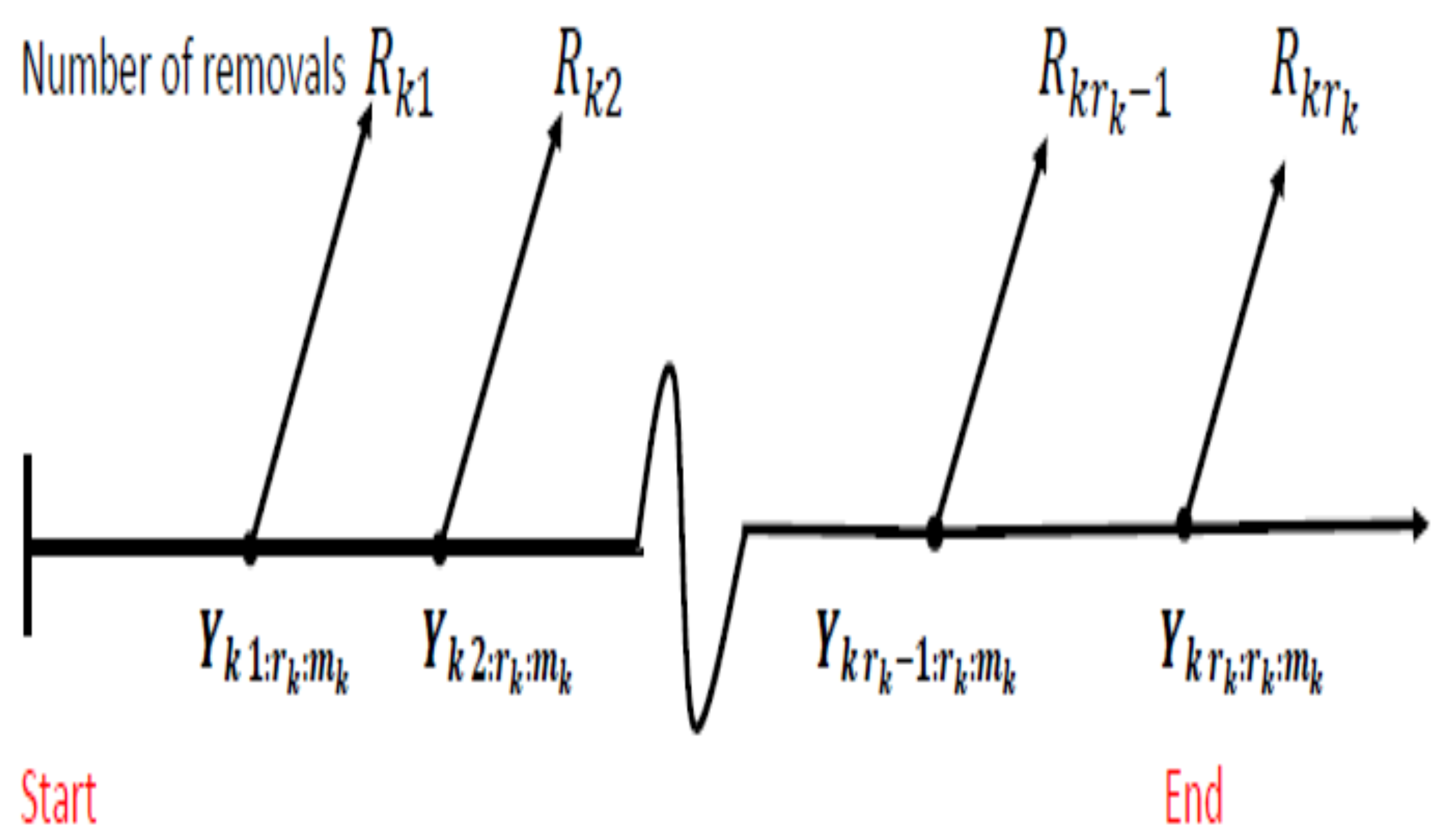
6.3. Progressive Type-II Censoring
6.4. Least Squares and Weighted Least Squares Estimations
6.5. Maximum Product of Spacing Estimation
7. Simulation Study
- Assign the values of and .
- The MLEs, MPSEs, LSEs, WLSEs, NACIs and LTCIs of the parameters and are computed as shown in Section 2.
- Evaluate the 95% NACIs and LTCIs of the parameters and .
- Repeat the above steps times.
- If is an estimate of , then the average of estimates, mean squared error (MSE) and relative absolute bias (RAB) of over ℏ samples are given, respectively, by
- Calculate the average of estimates of the parameters and and their MSEs and RABs as shown in Step 5. Calculate also the mean of the MSEs (MMSE) and mean of the RABs (MRAB) according to the following two relations:
- Calculate the average interval lengths (AILs) and coverage probability (COVP) of the parameters and .
- CS1: For
- CS2: For
- CS3: For
- In the case of two groups , we consider
- In the case of three groups , we consider
Numerical Results
- The MLEs are better than the LSEs and WLSEs through the AMSEs and ARABs;
- The MLEs are better than the MSPEs through the AMSEs and ARABs for the parameter ;
- The WLSEs are better than the LSEs through the AMSEs and ARABs;
- The MPSEs are better than the LSEs and WLSEs through the AMSEs;
- The NACLs are better than the LTCIs via the AILs and COVP;
- For , and fixed values of the total number of items to be tested, , and hence fixed sample sizes, , by increasing the failure times, , the MSEs, AMSEs, RABs, ARABs and AILs of the considered parameters decrease.
- For , and fixed values of the failure times, (=50%, 75% and of the sample size ), by increasing the total number of items to be tested, , the MSEs, AMSEs, RABs, ARABs and AILs of the considered parameters decrease.
- For fixing the total number of items to be tested, by increasing ℓ, the MSEs, AMSEs, RABs and ARABs decrease.
- By increasing the sample and failure time sizes (, ), the COVP are close to 95%.
- For fixed values of the sample and failure time sizes (, ), the third CS gives more accurate results through the MSEs, AMSEs, RABs, ARABs and AILs than the other two CSs.
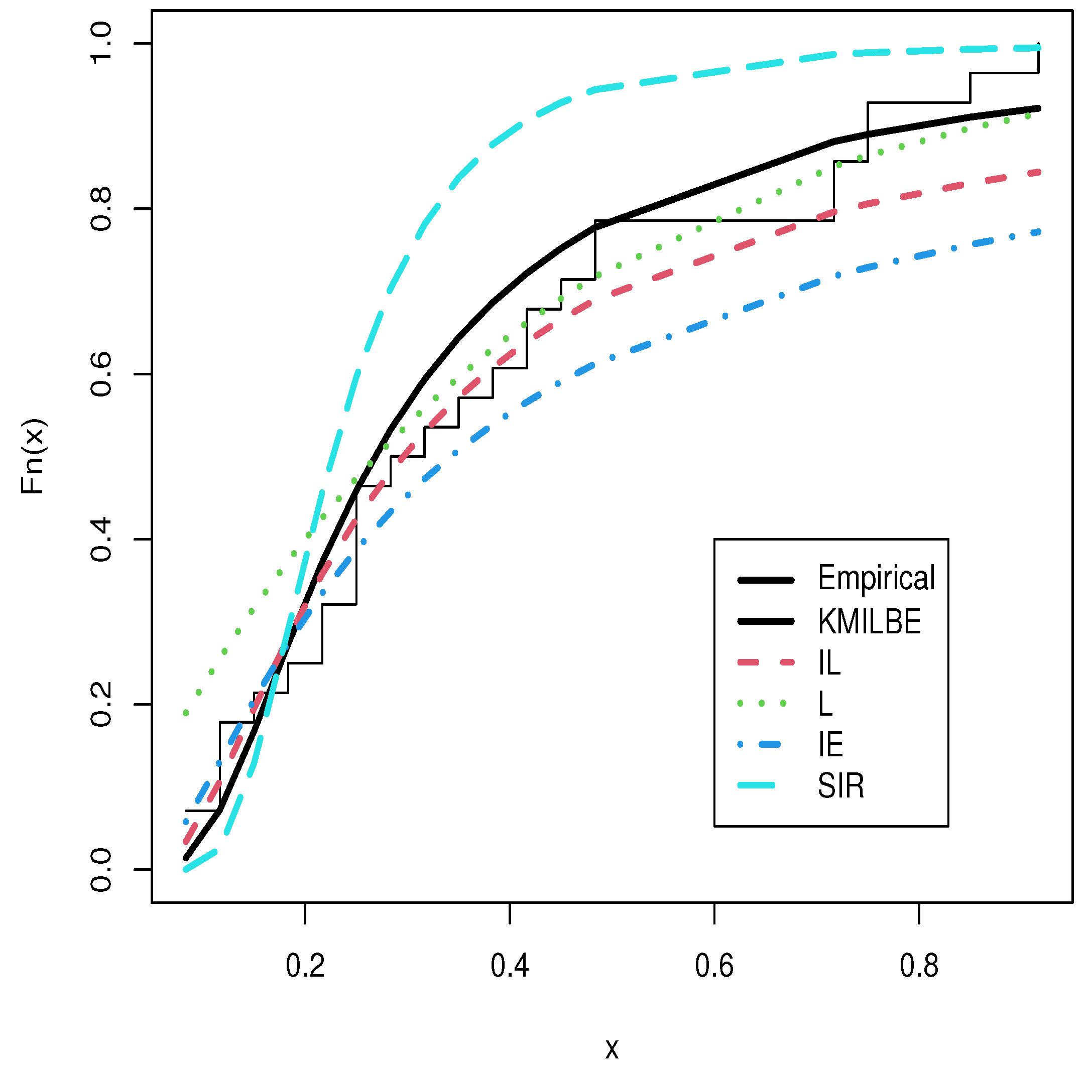
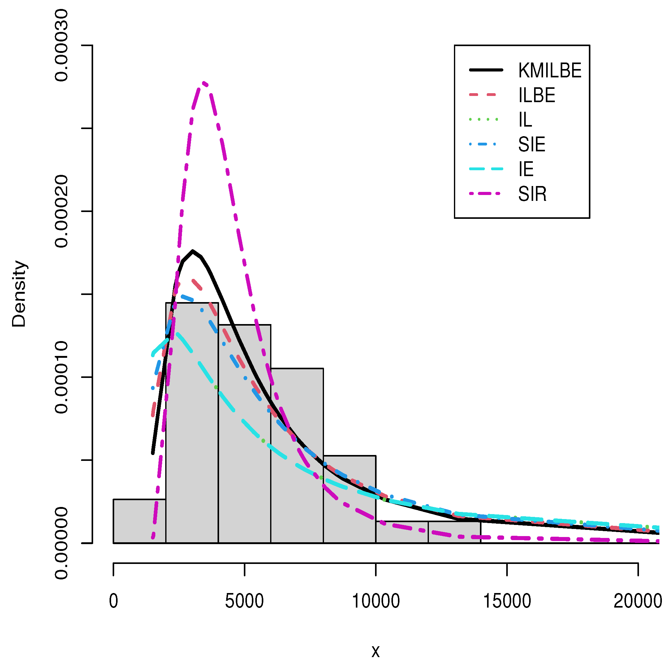
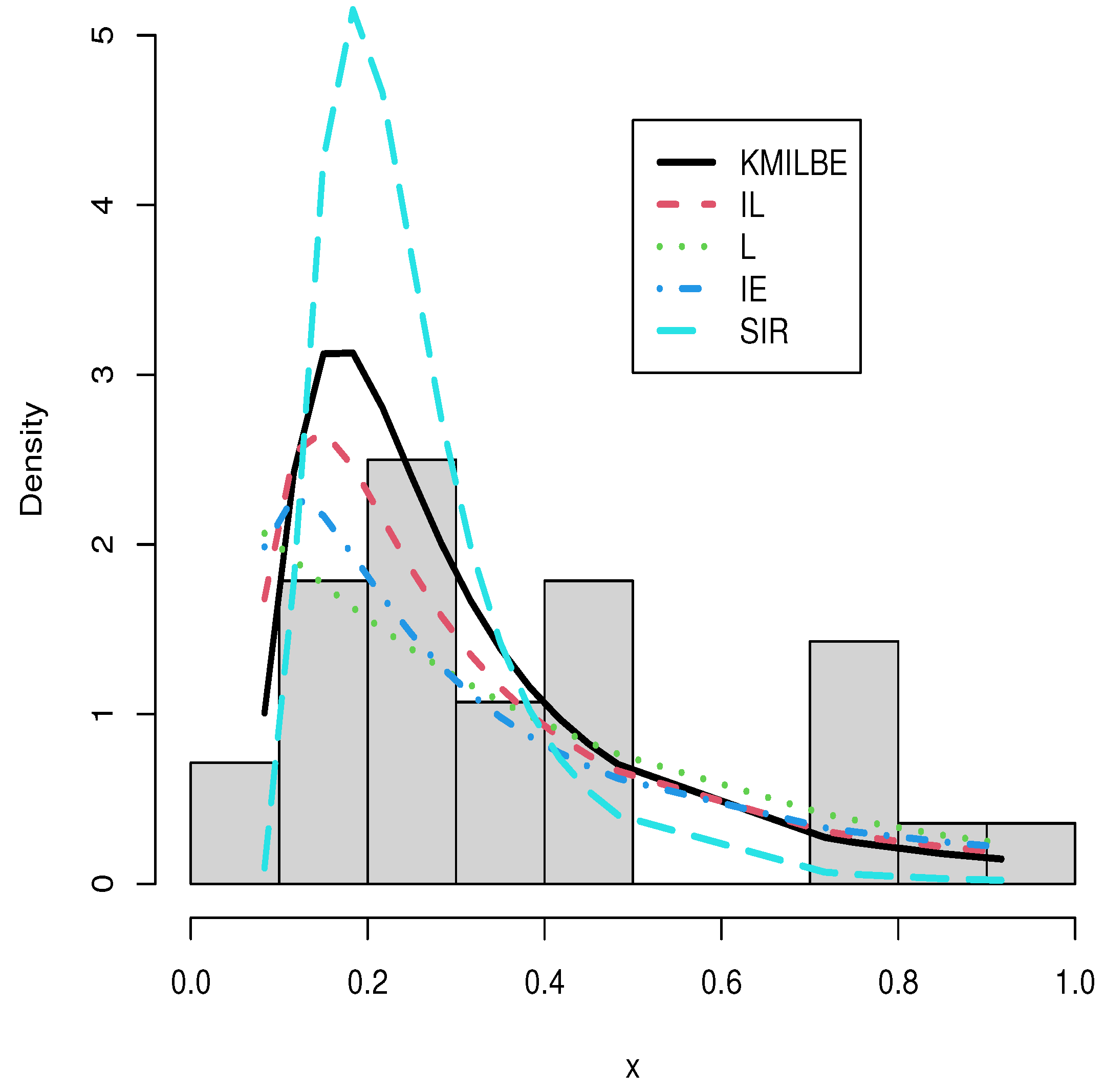
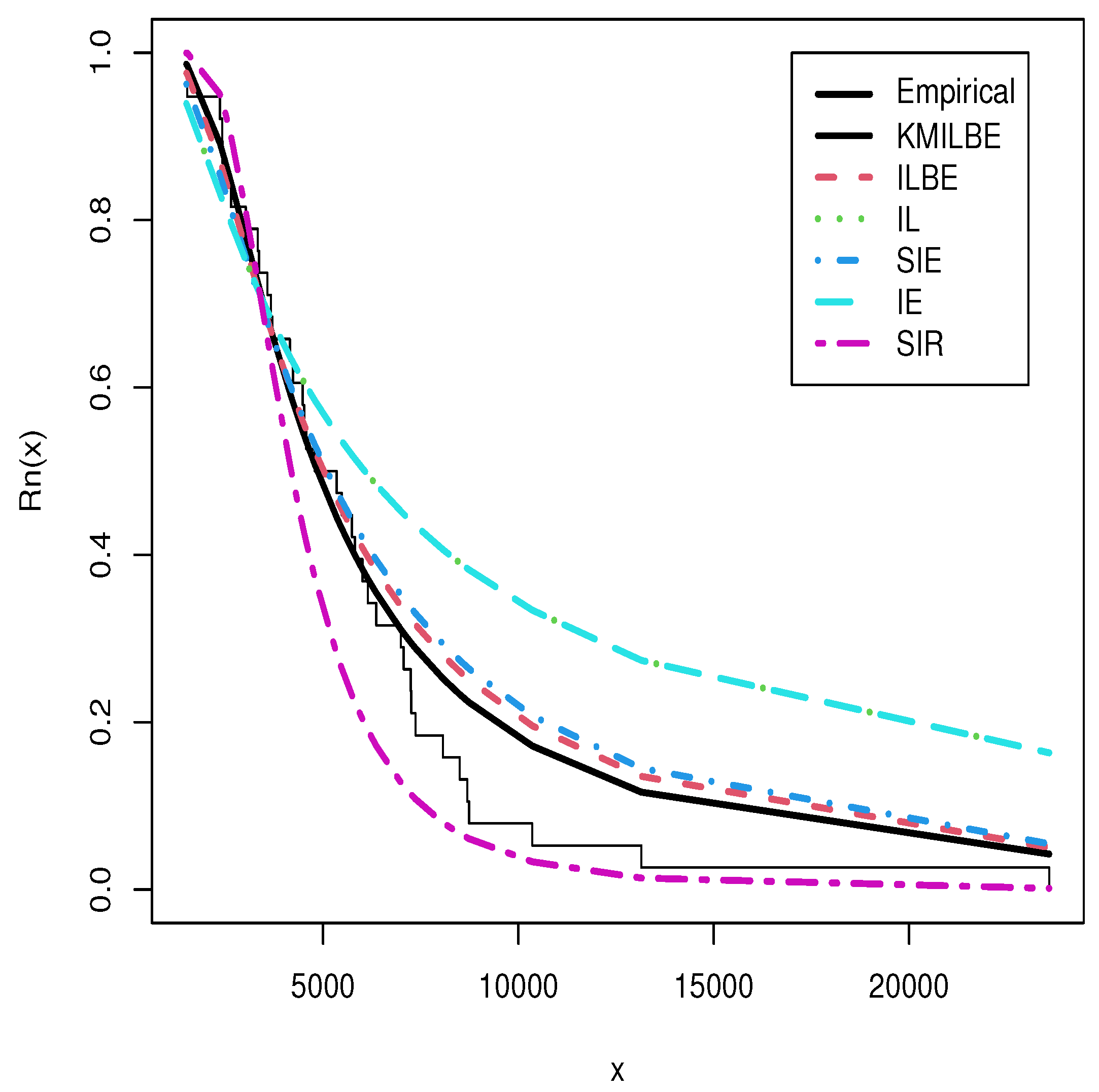
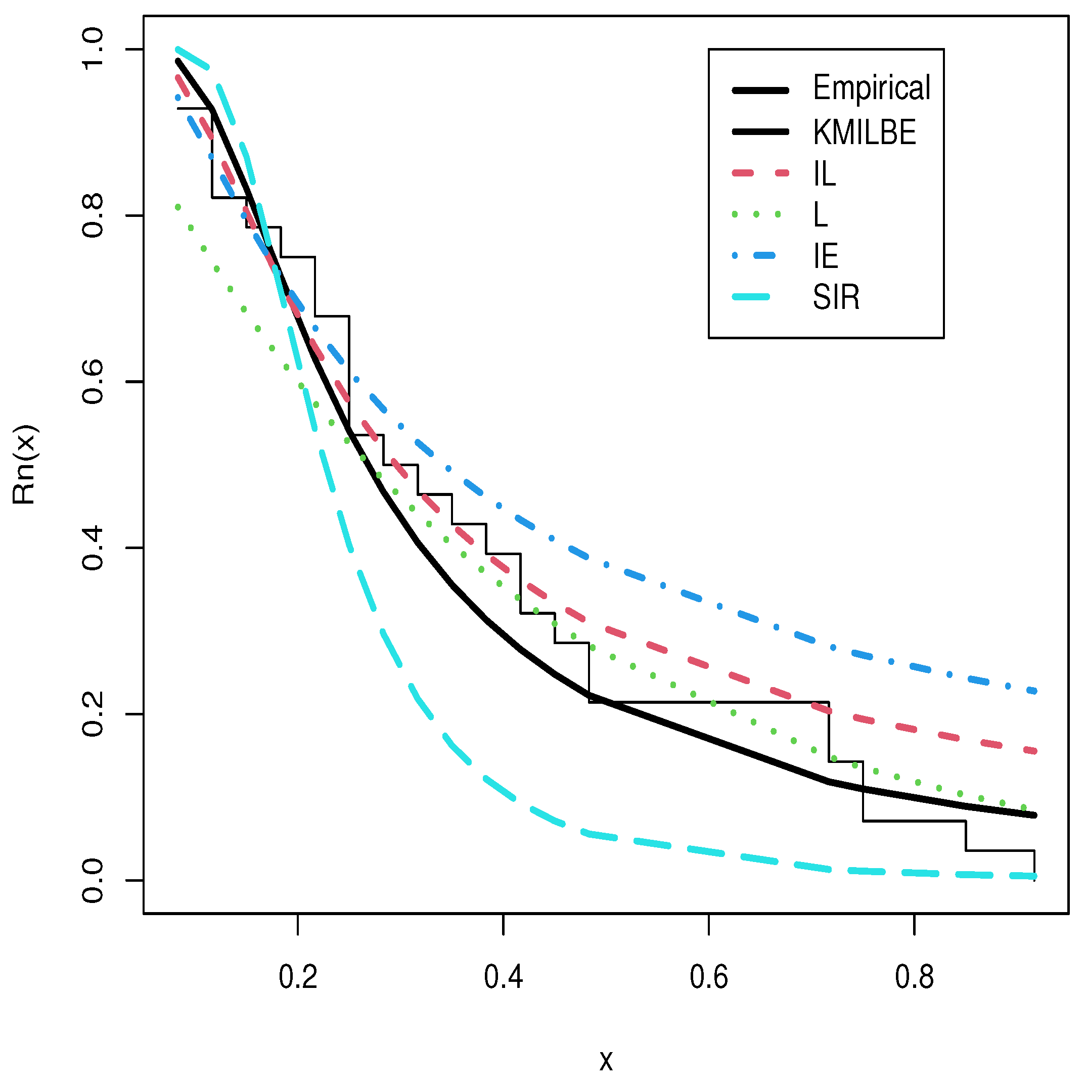
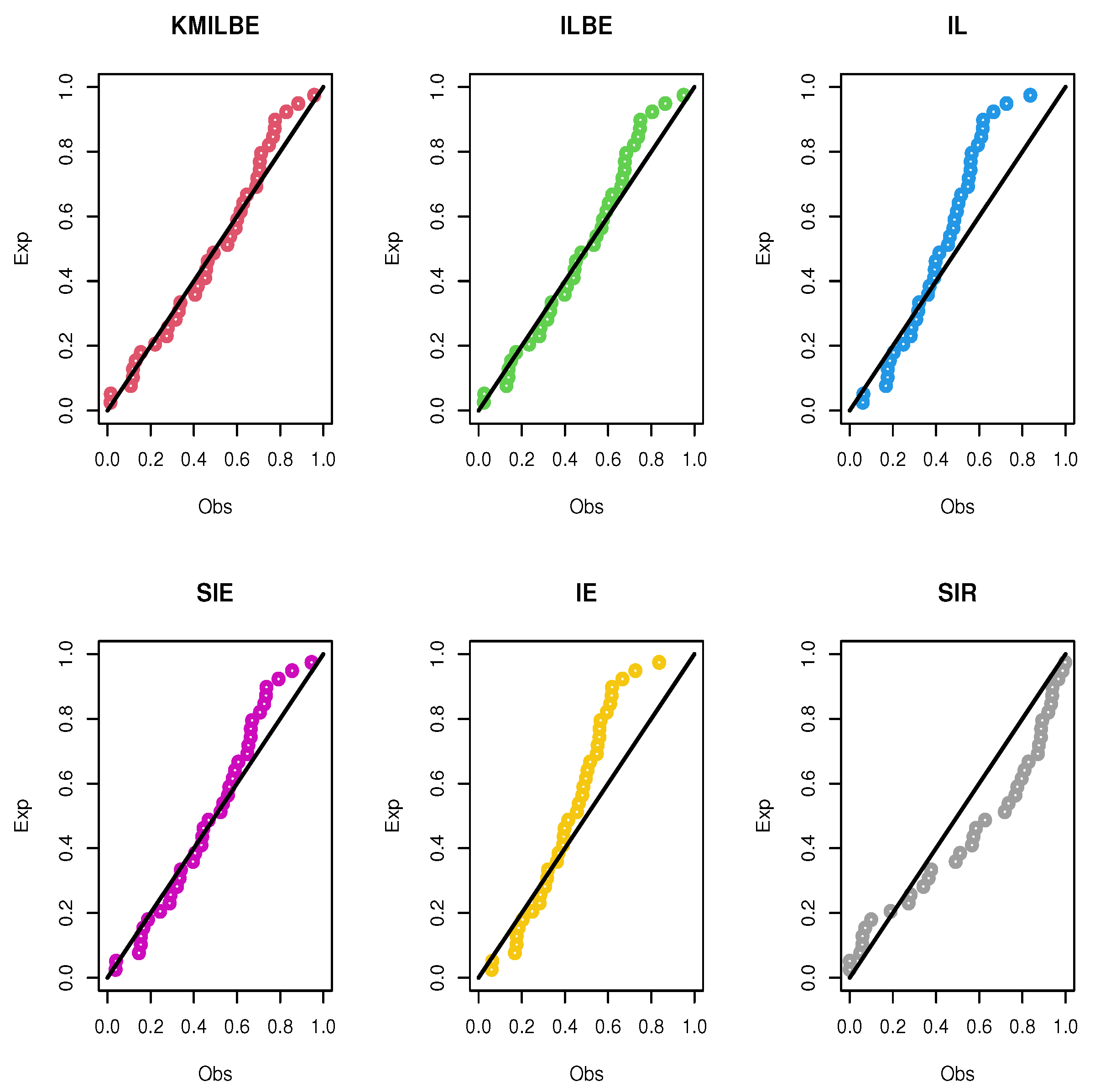
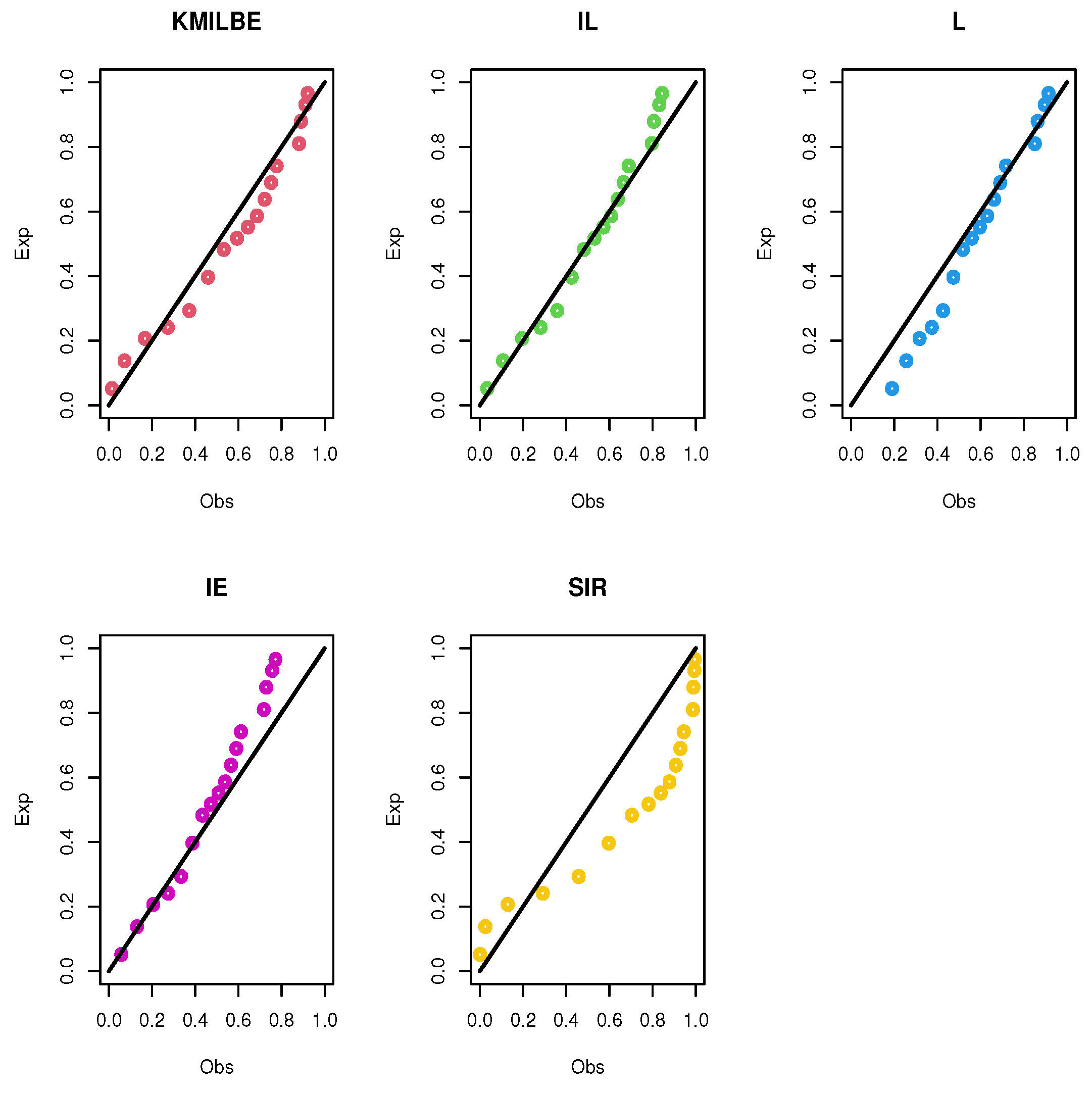
8. Real Data Analysis
9. Conclusions
Author Contributions
Funding
Informed Consent Statement
Data Availability Statement
Conflicts of Interest
References
- Nelson, N. Accelerated Testing: Statistical Models, Test Plans and Data Analysis; Wiley: New York, NY, USA, 1990. [Google Scholar]
- AL-Hussaini, E.K.; Abdel-Hamid, A.H. Bayesian estimation of the parameters, reliability and hazard rate functions of mixtures under accelerated life tests. Commun. Statist. Simul. Comput. 2004, 33, 963–982. [Google Scholar] [CrossRef]
- AL-Hussaini, E.K.; Abdel-Hamid, A.H. Accelerated life tests under finite mixture models. J. Statist. Comput. Simul. 2006, 76, 673–690. [Google Scholar] [CrossRef]
- Abdel-Hamid, A.H.; AL-Hussaini, E.K. Estimation in step-stress accelerated life tests for the exponentiated exponential distribution with type-I censoring. Comput. Statist. Data Anal. 2009, 53, 1328–1338. [Google Scholar] [CrossRef]
- Abdel-Hamid, A.H.; Hashem, A.F. Inference for the Exponential Distribution under Generalized Progressively Hybrid Censored Data from Partially Accelerated Life Tests with a Time Transformation Function. Mathematics 2021, 9, 1510. [Google Scholar] [CrossRef]
- Yin, X.K.; Sheng, B.Z. Some aspects of accelerated life testing by progressive stress. IEEE Trans. Reliab. 1987, 36, 150–155. [Google Scholar] [CrossRef]
- Abdel-Hamid, A.H.; AL-Hussaini, E.K. Bayesian prediction for type-II progressive-censored data from the Rayleigh distribution under progressive-stress model. J. Statist. Comput. Simul. 2014, 84, 1297–1312. [Google Scholar] [CrossRef]
- Abdel-Hamid, A.H.; Abushal, T.A. Inference on progressive-stress model for the exponentiated exponential distribution under type-II progressive hybrid censoring. J. Statist. Comput. Simul. 2015, 85, 1165–1186. [Google Scholar] [CrossRef]
- AL-Hussaini, E.K.; Abdel-Hamid, A.H.; Hashem, A.F. One-sample Bayesian prediction intervals based on progressively type-II censored data from the half-logistic distribution under progressive-stress model. Metrika 2015, 78, 771–783. [Google Scholar] [CrossRef]
- Nadarajah, S.; Abdel-Hamid, A.H.; Hashem, A.F. Inference for a geometric-Poisson-Rayleigh distribution under progressive-stress model based on type-I progressive hybrid censoring with binomial removals. Qual. Reliab. Eng. Int. 2018, 34, 649–680. [Google Scholar] [CrossRef]
- Mann, N.R.; Schafer, R.E.; Singpurwalla, N.D. Methods for Statistical Analysis of Reliability and Life Data; Wiley: New York, NY, USA, 1974. [Google Scholar]
- Meeker, W.Q.; Escobar, L.A. Statistical Methods for Reliability Data; Wiley: New York, NY, USA, 1998. [Google Scholar]
- Lawless, J.F. Statistical Models and Methods for Lifetime Data, 2nd ed.; Wiley: New York, NY, USA, 2003. [Google Scholar]
- Balakrishnan, N.; Sandhu, R.A. A simple simulation algorithm for generating progressive type-II censored samples. Am. Stat. 1995, 49, 229–230. [Google Scholar] [CrossRef]
- Aggarwala, R.; Balakrishnan, N. Some properties of progressive censored order statistics from arbitrary and uniform distributions with applications to inference and simulation. J. Stat. Plann. Inf. 1998, 70, 35–49. [Google Scholar] [CrossRef]
- Balakrishnan, N.; Aggarwala, R. Progressive Censoring: Theory, Methods, and Applications; Birkhäuser: Boston, MA, USA, 2000. [Google Scholar]
- Hashem, A.F.; Alyami, S.A. Inference on a New Lifetime Distribution under Progressive Type-II Censoring for a Parallel-Series structure. Complexity 2021, 2021, 6684918. [Google Scholar] [CrossRef]
- Marshall, A.; Olkin, I. A new method for adding a parameter to a class of distributions with applications to the exponential and Weibull families. Biometrika 1997, 84, 641–652. [Google Scholar] [CrossRef]
- Cordeiro, G.M.; De Castro, M. A new family of generalized distributions. J. Statist. Comput. Simul. 2011, 81, 883–893. [Google Scholar] [CrossRef]
- Cordeiro, G.M.; Afify, A.Z.; Ortega, E.M.M.; Suzuki, A.K.; Mead, M.E. The odd Lomax generator of distributions: Properties, estimation and applications. J. Comput. Appl. Math. 2019, 347, 222–237. [Google Scholar] [CrossRef]
- Kumar, D.; Singh, U.; Singh, S.K. A New distribution using Sine function- its application to bladder cancer patients data. J. Statist. App. Probab. 2015, 4, 417–427. [Google Scholar]
- Afify, A.Z.; Alizadeh, M. The odd Dagum family of distributions: Properties and applications. J. Appl. Probab. 2020, 15, 45–72. [Google Scholar]
- Hassan, A.S.; Elgarhy, M.; Shakil, M. Type II half-logistic class of distributions with applications. Pak. J. Stat. Oper. Res. 2017, 13, 245–264. [Google Scholar]
- Afify, A.Z.; Alizadeh, M.; Yousof, H.M.; Aryal, G.; Ahmad, M. The transmuted geometric-G family of distributions: Theory and applications. Pak. J. Statist. 2016, 32, 139–160. [Google Scholar]
- Elbatal, I.; Alotaibi, N.; Almetwally, E.M.; Alyami, S.A.; Elgarhy, M. On Odd Perks-G Class of Distributions: Properties, Regression Model, Discretization, Bayesian and Non-Bayesian Estimation, and Applications. Symmetry 2022, 14, 883. [Google Scholar] [CrossRef]
- Gomes, F.; Percontini, A.; De Brito, E.; Ramos, M.; Venancio, R.; Cordeiro, G. The odd Lindley-G family of distributions. Austrian J. Stat. 2017, 1, 57–79. [Google Scholar]
- Alotaibi, N.; Elbatal, I.; Almetwally, E.M.; Alyami, S.A.; Al-Moisheer, A.S.; Elgarhy, M. Truncated Cauchy Power Weibull-G Class of Distributions: Bayesian and Non-Bayesian Inference Modelling for COVID-19 and Carbon Fiber Data. Mathematics 2022, 10, 1565. [Google Scholar] [CrossRef]
- Nofal, Z.M.; Afify, A.Z.; Yousof, H.M.; Cordeiro, G.M. The generalized transmuted-G family of distributions. Commun. Stat. Theory Methods 2017, 46, 4119–4136. [Google Scholar] [CrossRef]
- Aldahlan, M.A.; Jamal, F.; Chesneau, C.; Elgarhy, M.; Elbatal, I. The truncated Cauchy power family of distributions with inference and applications. Entropy 2020, 22, 346. [Google Scholar] [CrossRef] [PubMed]
- Yousof, H.M.; Afify, A.Z.; Hamedani, G.G.; Aryal, G. The Burr X generator of distributions for lifetime data. J. Stat. Theory Appl. 2017, 16, 288–305. [Google Scholar] [CrossRef]
- Badr, M.; Elbatal, I.; Jamal, F.; Chesneau, C.; Elgarhy, M. The Transmuted Odd Fréchet-G class of Distributions: Theory and Applications. Mathematics 2020, 8, 958. [Google Scholar] [CrossRef]
- Al-Mofleh, H.; Elgarhy, M.; Afify, A.Z.; Zannon, M.S. Type II exponentiated half logistic generated family of distributions with applications. Electron. J. Appl. Stat. Anal. 2020, 13, 36–561. [Google Scholar]
- Al-Shomrani, A.; Arif, O.; Shawky, A.; Hanif, S.; Shahbaz, M.Q. Topp–Leone family of distributions: Some properties and application. Pak. J. Stat. Oper. Res. 2016, 12, 443–451. [Google Scholar] [CrossRef]
- Bantan, R.A.; Chesneau, C.; Jamal, F.; Elgarhy, M. On the analysis of new COVID-19 cases in Pakistan using an exponentiated version of the M family of distributions. Mathematics 2020, 8, 953. [Google Scholar] [CrossRef]
- Nascimento, A.; Silva, K.F.; Cordeiro, M.; Alizadeh, M.; Yousof, H.; Hamedani, G. The odd Nadarajah–Haghighi family of distributions. Prop. Appl. Stud. Sci. Math. Hung. 2019, 56, 1–26. [Google Scholar]
- Almarashi, A.M.; Jamal, F.; Chesneau, C.; Elgarhy, M. The Exponentiated truncated inverse Weibull-generated family of distributions with applications. Symmetry 2020, 12, 650. [Google Scholar] [CrossRef]
- Alzaatreh, A.; Lee, C.; Famoye, F. A new method for generating families of continuous distributions. Metron 2013, 71, 63–79. [Google Scholar] [CrossRef]
- Kumar, D.; Singh, U.; Singh, S.K. A method of proposing new distribution and its application to bladder cancer patients data. J. Statist. Appl. Probab. Lett. 2015, 2, 235–245. [Google Scholar]
- Maurya, S.K.; Kaushik, A.; Singh, S.K.; Singh, U. A new class of exponential transformed Lindley distribution and its application to Yarn data. Int. J. Statist. Econo. 2017, 18, 135–151. [Google Scholar]
- Kavya, P.; Manoharan, M. On a Generalized lifetime model using DUS transformation. In Applied Probability and Stochastic Processes; Joshua, V., Varadhan, S., Vishnevsky, V., Eds.; Infosys Science Foundation Series; Springer: Singapore, 2020; pp. 281–291. [Google Scholar]
- Kavya, P.; Manoharan, M. Some parsimonious models for lifetimes and applications. J. Statist. Comput. Simul. 2021, 91, 3693–3708. [Google Scholar] [CrossRef]
- Dara, T.; Ahmad, M. Recent Advances in Moment Distributions and Their Hazard Rate. Ph.D. Thesis, National College of Business Administration and Economics, Lahore, Pakistan, 2012. [Google Scholar]
- Almutiry, W. Inverted Length-Biased Exponential Model: Statistical Inference and Modeling. J. Math. 2021, 2021, 1980480. [Google Scholar] [CrossRef]
- Rényi, A. On measures of entropy and information. In Proceedings of the Fourth Berkeley Symposium on Mathematical Statistics and Probability, Volume 1: Contributions to the Theory of Statistics; Statistical Laboratory of the University of California: Berkeley, CA, USA, 1960; p. 767. [Google Scholar]
- Tsallis, C. Possible generalization of Boltzmann-Gibbs statistics. J. Statist. Phys. 1988, 52, 479–487. [Google Scholar] [CrossRef]
- Havrda, J.; Charvat, F. Quantification method of classification processes, concept of structural a-entropy. Kybernetika 1967, 3, 30–35. [Google Scholar]
- Arimoto, S. Information-theoretical considerations on estimation problems. Inf. Cont. 1971, 19, 181–194. [Google Scholar] [CrossRef]
- Lad, F.; Sanfilippo, G.; Agro, G. Extropy: Complementary dual of entropy. Stat. Sci. 2015, 30, 40–58. [Google Scholar] [CrossRef]
- Jahanshahi, S.; Zarei, H.; Khammar, A. On cumulative residual extropy. Probab. Eng. Inf. Sci. 2020, 34, 605–625. [Google Scholar] [CrossRef]
- Abdul Sathar, E.I.; Nair, D. On dynamic survival extropy. Commun. Stat.-Theory Methods 2020, 50, 1295–1313. [Google Scholar] [CrossRef]
- Swain, J.J.; Venkatraman, S.; Wilson, J.R. Least-squares estimation of distribution function in Johnson’s translation system. J. Statist. Comput. Simul. 1988, 29, 271–297. [Google Scholar] [CrossRef]
- Abdel-Hamid, A.H.; Hashem, A.F. A new lifetime distribution for a series-parallel system: Properties, applications and estimations under progressive type-II censoring. J. Statist. Comput. Simul. 2017, 87, 993–1024. [Google Scholar] [CrossRef]
- Cheng, R.C.H.; Amin, N.A.K. Estimating parameters in continuous univariate distributions with a shifted origin. J. the Roy. Statist. Soc. B 1983, 45, 394–403. [Google Scholar] [CrossRef]
- Ng, H.K.T.; Luo, L.; Hu, Y.; Duan, F. Parameter estimation of three-parameter Weibull distribution based on progressively type-II censored samples. J. Stat. Comput. Simul. 2012, 82, 1661–1678. [Google Scholar] [CrossRef]
- Ugarte, M.D.; Militino, A.; Arnholt, A.T. Probability and Statistics with R; Chapman & Hall: London, UK, 2008. [Google Scholar]
- Klein, J.P.; Moeschberger, M.L. Survival Analysis: Techniques for Censored and Truncated Data; Springer: Berlin/Heidelberg, Germany, 2006. [Google Scholar]

| MLE | MPSE | |||||||||||
|---|---|---|---|---|---|---|---|---|---|---|---|---|
| ⋮ | ⋮ | MSE() | RAB() | AMSE | MSE() | RAB() | AMSE | |||||
| ℓ | CS | MSE() | RAB() | ARAB | MSE() | RAB() | ARAB | |||||
| 60 | 2 | 30 | 15 | I | 1.53024 | 0.05812 | 0.12577 | 0.03379 | 1.48487 | 0.04614 | 0.11121 | 0.02773 |
| 30 | 15 | 0.22606 | 0.00947 | 0.37923 | 0.25250 | 0.16227 | 0.00932 | 0.40166 | 0.25644 | |||
| II | 1.53595 | 0.04652 | 0.11181 | 0.02743 | 1.48572 | 0.0377 | 0.10132 | 0.02280 | ||||
| 0.22546 | 0.00834 | 0.35354 | 0.23268 | 0.17043 | 0.0079 | 0.36371 | 0.23251 | |||||
| III | 1.52858 | 0.04054 | 0.10481 | 0.02420 | 1.50566 | 0.03521 | 0.09698 | 0.02144 | ||||
| 0.22350 | 0.00785 | 0.34484 | 0.22482 | 0.18206 | 0.00768 | 0.35259 | 0.22478 | |||||
| 22 | I | 1.52152 | 0.04256 | 0.10759 | 0.02494 | 1.47824 | 0.03525 | 0.09856 | 0.02143 | |||
| 22 | 0.22143 | 0.00731 | 0.33167 | 0.21963 | 0.16431 | 0.00761 | 0.35809 | 0.22832 | ||||
| II | 1.52260 | 0.03679 | 0.10087 | 0.02184 | 1.48067 | 0.03044 | 0.09125 | 0.01886 | ||||
| 0.22222 | 0.00688 | 0.32683 | 0.21385 | 0.16661 | 0.00729 | 0.34808 | 0.21966 | |||||
| III | 1.52217 | 0.03461 | 0.09761 | 0.02055 | 1.50056 | 0.02943 | 0.08901 | 0.01808 | ||||
| 0.22000 | 0.00649 | 0.31635 | 0.20698 | 0.17947 | 0.00672 | 0.33085 | 0.20993 | |||||
| 30 | 1.5168 | 0.03236 | 0.09332 | 0.01928 | 1.47735 | 0.02745 | 0.08799 | 0.01709 | ||||
| 30 | 0.21873 | 0.0062 | 0.30563 | 0.19948 | 0.16573 | 0.00672 | 0.33395 | 0.21097 | ||||
| 3 | 20 | 10 | I | 1.50363 | 0.03188 | 0.09438 | 0.01999 | 1.51203 | 0.02856 | 0.08792 | 0.01866 | |
| 20 | 10 | 0.22289 | 0.00810 | 0.35086 | 0.22262 | 0.15476 | 0.00875 | 0.38819 | 0.23806 | |||
| 20 | 10 | 2 | 1.50703 | 0.02563 | 0.08418 | 0.01633 | 1.50139 | 0.02327 | 0.07961 | 0.01546 | ||
| 0.22049 | 0.00704 | 0.32220 | 0.20319 | 0.16055 | 0.00765 | 0.35851 | 0.21906 | |||||
| III | 1.50395 | 0.02286 | 0.08027 | 0.01485 | 1.51370 | 0.02116 | 0.07502 | 0.01396 | ||||
| 0.22105 | 0.00685 | 0.32158 | 0.20093 | 0.17491 | 0.00675 | 0.33257 | 0.20380 | |||||
| 15 | I | 1.49880 | 0.02440 | 0.08310 | 0.01544 | 1.50236 | 0.02143 | 0.07688 | 0.01451 | |||
| 15 | 0.21841 | 0.00648 | 0.31646 | 0.19978 | 0.15325 | 0.00758 | 0.35827 | 0.21757 | ||||
| 15 | 2 | 1.49920 | 0.02138 | 0.07757 | 0.01355 | 1.50050 | 0.01861 | 0.07160 | 0.01273 | |||
| 0.21803 | 0.00572 | 0.29586 | 0.18671 | 0.16032 | 0.00685 | 0.33739 | 0.20449 | |||||
| III | 1.49764 | 0.02039 | 0.07561 | 0.01307 | 1.51345 | 0.01954 | 0.07235 | 0.01301 | ||||
| 0.21837 | 0.00575 | 0.29681 | 0.18621 | 0.17124 | 0.00649 | 0.32721 | 0.19978 | |||||
| 20 | 1.49669 | 0.01886 | 0.07293 | 0.01200 | 1.50042 | 0.01721 | 0.06919 | 0.01179 | ||||
| 20 | 0.21724 | 0.00514 | 0.28210 | 0.17752 | 0.15833 | 0.00638 | 0.32664 | 0.19791 | ||||
| 20 | ||||||||||||
| 120 | 2 | 60 | 30 | I | 1.51388 | 0.02722 | 0.08678 | 0.01597 | 1.47963 | 0.02448 | 0.08100 | 0.01534 |
| 60 | 30 | 0.21869 | 0.00471 | 0.26997 | 0.17837 | 0.16768 | 0.00619 | 0.31628 | 0.19864 | |||
| II | 1.51637 | 0.02148 | 0.07706 | 0.01271 | 1.48762 | 0.01830 | 0.07010 | 0.01177 | ||||
| 0.21666 | 0.00393 | 0.24826 | 0.16266 | 0.17449 | 0.00524 | 0.28384 | 0.17697 | |||||
| III | 1.51164 | 0.01922 | 0.07291 | 0.01148 | 1.49763 | 0.01640 | 0.06653 | 0.01077 | ||||
| 0.21586 | 0.00374 | 0.23947 | 0.15619 | 0.18138 | 0.00514 | 0.28047 | 0.17350 | |||||
| 45 | I | 1.51019 | 0.02027 | 0.07529 | 0.01200 | 1.48076 | 0.01728 | 0.06912 | 0.01125 | |||
| 45 | 0.21642 | 0.00372 | 0.24067 | 0.15798 | 0.17127 | 0.00523 | 0.28429 | 0.17671 | ||||
| II | 1.51018 | 0.01693 | 0.06818 | 0.01010 | 1.48194 | 0.01505 | 0.06404 | 0.01001 | ||||
| 0.21462 | 0.00327 | 0.22335 | 0.14577 | 0.17236 | 0.00497 | 0.27479 | 0.16941 | |||||
| III | 1.50822 | 0.01656 | 0.06806 | 0.00987 | 1.49334 | 0.01430 | 0.06195 | 0.00952 | ||||
| 0.21470 | 0.00319 | 0.22292 | 0.14549 | 0.17905 | 0.00474 | 0.26336 | 0.16266 | |||||
| 60 | 1.50503 | 0.01562 | 0.06583 | 0.00925 | 1.48008 | 0.01354 | 0.06086 | 0.00913 | ||||
| 60 | 0.21199 | 0.00287 | 0.21081 | 0.13832 | 0.17163 | 0.00472 | 0.26401 | 0.16244 | ||||
| 3 | 40 | 20 | I | 1.50019 | 0.01744 | 0.06979 | 0.01076 | 1.49627 | 0.01484 | 0.06316 | 0.01029 | |
| 40 | 20 | 0.21572 | 0.00408 | 0.25050 | 0.16015 | 0.16160 | 0.00575 | 0.30320 | 0.18318 | |||
| 40 | 20 | II | 1.49748 | 0.01228 | 0.05844 | 0.00778 | 1.49558 | 0.01157 | 0.05601 | 0.00841 | ||
| 0.21360 | 0.00328 | 0.22342 | 0.14093 | 0.16736 | 0.00525 | 0.28359 | 0.16980 | |||||
| III | 1.4987 | 0.01120 | 0.05564 | 0.00720 | 1.50436 | 0.00994 | 0.05191 | 0.00728 | ||||
| 0.2133 | 0.00319 | 0.22129 | 0.13846 | 0.17736 | 0.00461 | 0.26034 | 0.15613 | |||||
| 30 | I | 1.49569 | 0.01219 | 0.05919 | 0.00766 | 1.49418 | 0.01038 | 0.05378 | 0.00773 | |||
| 30 | 0.21293 | 0.00313 | 0.22087 | 0.14003 | 0.16353 | 0.00509 | 0.27838 | 0.16608 | ||||
| 30 | II | 1.49822 | 0.01053 | 0.05469 | 0.00672 | 1.4964 | 0.00948 | 0.05092 | 0.00708 | |||
| 0.21248 | 0.00290 | 0.21068 | 0.13269 | 0.16804 | 0.00467 | 0.2659 | 0.15841 | |||||
| III | 1.49773 | 0.01023 | 0.05395 | 0.00649 | 1.50444 | 0.00910 | 0.05000 | 0.00671 | ||||
| 0.21282 | 0.00275 | 0.20591 | 0.12993 | 0.17605 | 0.00432 | 0.24853 | 0.14926 | |||||
| 40 | 1.49504 | 0.01006 | 0.05334 | 0.00631 | 1.49543 | 0.00879 | 0.04926 | 0.00665 | ||||
| 40 | 0.21165 | 0.00255 | 0.19737 | 0.12535 | 0.16808 | 0.00452 | 0.25882 | 0.15404 | ||||
| 40 | ||||||||||||
| LSE | WLSE | |||||||||||
|---|---|---|---|---|---|---|---|---|---|---|---|---|
| ⋮ | ⋮ | MSE() | RAB() | AMSE | MSE() | RAB() | AMSE | |||||
| ℓ | CS | MSE() | RAB() | ARAB | MSE() | RAB() | ARAB | |||||
| 60 | 2 | 30 | 15 | I | 1.53847 | 0.06934 | 0.13439 | 0.04335 | 1.53427 | 0.06331 | 0.12874 | 0.03884 |
| 30 | 15 | 0.21641 | 0.01736 | 0.50731 | 0.32085 | 0.21840 | 0.01438 | 0.45715 | 0.29294 | |||
| II | 1.51732 | 0.05361 | 0.12044 | 0.03249 | 1.52090 | 0.04666 | 0.11150 | 0.02780 | ||||
| 0.20097 | 0.01137 | 0.41966 | 0.27005 | 0.20462 | 0.00895 | 0.36927 | 0.24038 | |||||
| III | 1.51425 | 0.0442 | 0.10963 | 0.02708 | 1.50998 | 0.04372 | 0.10925 | 0.02647 | ||||
| 0.20677 | 0.00995 | 0.3902 | 0.24992 | 0.20583 | 0.00921 | 0.37535 | 0.24230 | |||||
| 22 | I | 1.51872 | 0.04514 | 0.11151 | 0.02837 | 1.5190 | 0.04271 | 0.10857 | 0.02636 | |||
| 22 | 0.20633 | 0.01159 | 0.42440 | 0.26795 | 0.2079 | 0.01000 | 0.39299 | 0.25078 | ||||
| II | 1.51972 | 0.04161 | 0.10676 | 0.02550 | 1.52121 | 0.04005 | 0.10449 | 0.02426 | ||||
| 0.20480 | 0.00940 | 0.38083 | 0.24380 | 0.20696 | 0.00848 | 0.35906 | 0.23178 | |||||
| III | 1.50950 | 0.03620 | 0.09975 | 0.02273 | 1.50629 | 0.03527 | 0.09861 | 0.02178 | ||||
| 0.20400 | 0.00926 | 0.37892 | 0.23933 | 0.20386 | 0.00829 | 0.35898 | 0.22880 | |||||
| 30 | 1.50890 | 0.03486 | 0.09826 | 0.02191 | 1.51050 | 0.03348 | 0.09626 | 0.02068 | ||||
| 30 | 0.20234 | 0.00896 | 0.37656 | 0.23741 | 0.20341 | 0.00788 | 0.35227 | 0.22426 | ||||
| 3 | 20 | 10 | I | 1.52104 | 0.04246 | 0.10806 | 0.02890 | 1.50653 | 0.03738 | 0.10193 | 0.02512 | |
| 20 | 10 | 0.20537 | 0.01533 | 0.47209 | 0.29008 | 0.20908 | 0.01286 | 0.42851 | 0.26522 | |||
| 20 | 10 | II | 1.51030 | 0.03455 | 0.09766 | 0.02251 | 1.49004 | 0.02921 | 0.09036 | 0.01872 | ||
| 0.19596 | 0.01046 | 0.39092 | 0.24429 | 0.19404 | 0.00822 | 0.34719 | 0.21878 | |||||
| III | 1.48314 | 0.02389 | 0.08204 | 0.01606 | 1.47306 | 0.02442 | 0.08327 | 0.01615 | ||||
| 0.19524 | 0.00822 | 0.36154 | 0.22179 | 0.19357 | 0.00788 | 0.35240 | 0.21783 | |||||
| 15 | I | 1.50977 | 0.02822 | 0.08836 | 0.01917 | 1.50605 | 0.02678 | 0.08647 | 0.01791 | |||
| 15 | 0.19966 | 0.01012 | 0.39540 | 0.24188 | 0.20258 | 0.00904 | 0.37310 | 0.22979 | ||||
| 15 | II | 1.50582 | 0.02343 | 0.08074 | 0.01564 | 1.49757 | 0.02276 | 0.07976 | 0.01501 | |||
| 0.19376 | 0.00784 | 0.35263 | 0.21669 | 0.19517 | 0.00726 | 0.33572 | 0.20774 | |||||
| III | 1.49938 | 0.02156 | 0.07803 | 0.01460 | 1.49095 | 0.02106 | 0.07719 | 0.01403 | ||||
| 0.19593 | 0.00764 | 0.34721 | 0.21262 | 0.19556 | 0.00701 | 0.33306 | 0.20513 | |||||
| 20 | 1.50700 | 0.02206 | 0.07825 | 0.01481 | 1.50702 | 0.02142 | 0.07711 | 0.01415 | ||||
| 20 | 0.19666 | 0.00756 | 0.34261 | 0.21043 | 0.19928 | 0.00687 | 0.32573 | 0.20142 | ||||
| 20 | ||||||||||||
| 120 | 2 | 60 | 30 | I | 1.51221 | 0.03432 | 0.09742 | 0.02172 | 1.51203 | 0.03227 | 0.09424 | 0.01989 |
| 60 | 30 | 0.20471 | 0.00912 | 0.37327 | 0.23535 | 0.20724 | 0.00751 | 0.33737 | 0.21581 | |||
| II | 1.50383 | 0.02803 | 0.08824 | 0.01702 | 1.50708 | 0.02329 | 0.08049 | 0.01389 | ||||
| 0.19879 | 0.00602 | 0.30803 | 0.19813 | 0.20184 | 0.00449 | 0.26468 | 0.17259 | |||||
| III | 1.50401 | 0.02067 | 0.07548 | 0.01277 | 1.50113 | 0.02053 | 0.07543 | 0.01249 | ||||
| 0.20108 | 0.00487 | 0.27445 | 0.17497 | 0.20094 | 0.00446 | 0.26372 | 0.16958 | |||||
| 45 | I | 1.50642 | 0.02376 | 0.08115 | 0.01496 | 1.50792 | 0.02239 | 0.07868 | 0.01380 | |||
| 45 | 0.20144 | 0.00617 | 0.30848 | 0.19481 | 0.20340 | 0.00522 | 0.28293 | 0.18080 | ||||
| II | 1.50260 | 0.01915 | 0.07324 | 0.01181 | 1.50436 | 0.01848 | 0.07197 | 0.01118 | ||||
| 0.19922 | 0.00447 | 0.26620 | 0.16972 | 0.20141 | 0.00389 | 0.24736 | 0.15967 | |||||
| III | 1.50569 | 0.01812 | 0.07102 | 0.01141 | 1.50349 | 0.01764 | 0.07005 | 0.01091 | ||||
| 0.20304 | 0.00469 | 0.27226 | 0.17164 | 0.20301 | 0.00417 | 0.25616 | 0.16310 | |||||
| 60 | 1.50372 | 0.01729 | 0.06921 | 0.01083 | 1.50533 | 0.01641 | 0.06756 | 0.01007 | ||||
| 60 | 0.19946 | 0.00437 | 0.26068 | 0.16495 | 0.20098 | 0.00373 | 0.24079 | 0.15418 | ||||
| 3 | 40 | 20 | I | 1.50804 | 0.02143 | 0.07695 | 0.01448 | 1.50185 | 0.01968 | 0.07387 | 0.01306 | |
| 40 | 20 | 0.19946 | 0.00754 | 0.34122 | 0.20908 | 0.20384 | 0.00644 | 0.31336 | 0.19362 | |||
| 40 | 20 | II | 1.50454 | 0.01655 | 0.06833 | 0.01085 | 1.49144 | 0.01384 | 0.06264 | 0.00881 | ||
| 0.19540 | 0.00515 | 0.28233 | 0.17533 | 0.19518 | 0.00378 | 0.24437 | 0.15350 | |||||
| III | 1.49479 | 0.01226 | 0.05832 | 0.00818 | 1.48801 | 0.01245 | 0.05902 | 0.00814 | ||||
| 0.19821 | 0.00411 | 0.25513 | 0.15673 | 0.19759 | 0.00383 | 0.24634 | 0.15268 | |||||
| 30 | I | 1.50478 | 0.01463 | 0.06361 | 0.00989 | 1.50278 | 0.01389 | 0.06186 | 0.00919 | |||
| 30 | 0.19803 | 0.00516 | 0.28418 | 0.17390 | 0.20082 | 0.00449 | 0.26447 | 0.16316 | ||||
| 30 | II | 1.50127 | 0.012 | 0.05802 | 0.00791 | 1.49621 | 0.01153 | 0.05699 | 0.00746 | |||
| 0.19636 | 0.00382 | 0.24638 | 0.1522 | 0.19791 | 0.00339 | 0.2318 | 0.14439 | |||||
| III | 1.49731 | 0.01125 | 0.05630 | 0.00757 | 1.49163 | 0.01099 | 0.05566 | 0.00724 | ||||
| 0.19674 | 0.00388 | 0.24655 | 0.15142 | 0.19681 | 0.00348 | 0.23349 | 0.14457 | |||||
| 40 | 1.50099 | 0.01069 | 0.05489 | 0.00723 | 1.50081 | 0.01036 | 0.05405 | 0.00684 | ||||
| 40 | 0.19907 | 0.00376 | 0.24161 | 0.14825 | 0.20116 | 0.00331 | 0.22620 | 0.14013 | ||||
| 40 | ||||||||||||
| NACI | LTCI | |||||||||
|---|---|---|---|---|---|---|---|---|---|---|
| ⋮ | ⋮ | CI() | AIL() | COVP() | CI() | AIL() | COVP() | |||
| ℓ | CS | CI() | AIL() | COVP() | CI() | AIL() | COVP() | |||
| 60 | 2 | 30 | 15 | I | (1.0616,1.9988) | 0.9372 | 95.38 | (1.1268,2.0788) | 0.9521 | 96.04 |
| 30 | 15 | (0.0512,0.4167) | 0.3655 | 96.50 | (0.1017,0.6088) | 0.5071 | 91.40 | |||
| II | (1.1249, 1.9470) | 0.8221 | 95.52 | (1.1754, 2.0074) | 0.8320 | 95.02 | ||||
| (0.0631, 0.3969) | 0.3337 | 94.92 | (0.1090, 0.5386) | 0.4296 | 90.70 | |||||
| III | (1.1427, 1.9144) | 0.7717 | 95.22 | (1.1876, 1.9676) | 0.7800 | 94.80 | ||||
| (0.0652, 0.3898) | 0.3246 | 95.12 | (0.1095, 0.5157) | 0.4062 | 90.88 | |||||
| 22 | I | (1.1251, 1.9179) | 0.7928 | 95.02 | (1.1726, 1.9745) | 0.8018 | 94.94 | |||
| 22 | (0.0627, 0.3879) | 0.3252 | 95.28 | (0.1076, 0.5202) | 0.4126 | 91.58 | ||||
| II | (1.1532, 1.8920) | 0.7389 | 95.26 | (1.1946, 1.9408) | 0.7462 | 95.30 | ||||
| (0.0699, 0.3803) | 0.3103 | 95.52 | (0.1119, 0.4848) | 0.3729 | 91.66 | |||||
| III | (1.1632, 1.8811) | 0.7179 | 94.82 | (1.2025, 1.9270) | 0.7246 | 95.04 | ||||
| (0.0697, 0.3757) | 0.3060 | 95.70 | (0.1111, 0.4778) | 0.3667 | 91.96 | |||||
| 30 | (1.1722, 1.8614) | 0.6892 | 94.42 | (1.2086, 1.9037) | 0.6952 | 94.28 | ||||
| 30 | (0.0745, 0.3670) | 0.2925 | 94.64 | (0.1135, 0.4585) | 0.3450 | 91.52 | ||||
| 3 | 20 | 10 | I | (1.1476, 1.8597) | 0.7121 | 94.74 | (1.1867, 1.9055) | 0.7188 | 95.52 | |
| 20 | 10 | (0.0591, 0.3970) | 0.3379 | 95.76 | (0.1057, 0.5599) | 0.4542 | 91.40 | |||
| 20 | 10 | II | (1.1932, 1.8209) | 0.6277 | 94.96 | (1.2237, 1.8560) | 0.6322 | 95.34 | ||
| (0.0682, 0.3785) | 0.3103 | 95.04 | (0.1105, 0.4733) | 0.3628 | 91.18 | |||||
| III | (1.2102, 1.7977) | 0.5876 | 94.18 | (1.2371, 1.8284) | 0.5913 | 94.96 | ||||
| (0.0730, 0.3739) | 0.3009 | 94.94 | (0.1133, 0.4640) | 0.3507 | 90.60 | |||||
| 15 | I | (1.1930, 1.8046) | 0.6116 | 94.28 | (1.2222, 1.8381) | 0.6159 | 94.80 | |||
| 15 | (0.0708, 0.3710) | 0.3002 | 95.38 | (0.1112, 0.4604) | 0.3492 | 91.94 | ||||
| 15 | II | (1.2145, 1.7838) | 0.5693 | 94.06 | (1.2400, 1.8127) | 0.5727 | 94.46 | |||
| (0.0758, 0.3636) | 0.2878 | 95.32 | (0.1141, 0.4402) | 0.3261 | 92.26 | |||||
| III | (1.2197, 1.7756) | 0.5558 | 94.10 | (1.2440, 1.8030) | 0.5590 | 94.64 | ||||
| (0.0776, 0.3622) | 0.2846 | 95.30 | (0.1152, 0.4347) | 0.3195 | 91.70 | |||||
| 20 | (1.2241, 1.7692) | 0.5451 | 94.90 | (1.2475, 1.7957) | 0.5481 | 95.36 | ||||
| 20 | (0.0815, 0.3552) | 0.2737 | 95.70 | (0.1170, 0.4196) | 0.3026 | 91.94 | ||||
| 20 | ||||||||||
| 120 | 2 | 60 | 30 | I | (1.1820, 1.8457) | 0.6637 | 95.70 | (1.2159, 1.8850) | 0.6690 | 95.52 |
| 60 | 30 | (0.0835, 0.3554) | 0.2719 | 95.88 | (0.1186, 0.4170) | 0.2984 | 93.08 | |||
| II | (1.2295, 1.8033) | 0.5738 | 95.78 | (1.2550, 1.8322) | 0.5773 | 95.58 | ||||
| (0.0966, 0.3373) | 0.2407 | 95.42 | (0.1253, 0.3826) | 0.2573 | 92.22 | |||||
| III | (1.2429, 1.7804) | 0.5376 | 95.22 | (1.2654, 1.8058) | 0.5404 | 94.98 | ||||
| (0.0992, 0.3329) | 0.2337 | 94.96 | (0.1266, 0.3752) | 0.2486 | 92.24 | |||||
| 45 | I | (1.2339, 1.7864) | 0.5525 | 95.06 | (1.2577, 1.8134) | 0.5556 | 95.12 | |||
| 45 | (0.0996, 0.3336) | 0.2340 | 95.24 | (0.1270, 0.3756) | 0.2486 | 92.10 | ||||
| II | (1.2534, 1.7669) | 0.5135 | 95.08 | (1.2741, 1.7901) | 0.5160 | 95.12 | ||||
| (0.1043, 0.3252) | 0.2209 | 95.26 | (0.1291, 0.3622) | 0.2331 | 92.88 | |||||
| III | (1.2584, 1.758) | 0.4996 | 94.96 | (1.2780, 1.7799) | 0.5019 | 94.86 | ||||
| (0.1055, 0.324) | 0.2185 | 95.40 | (0.1298, 0.3599) | 0.2301 | 92.46 | |||||
| 60 | (1.2638, 1.7462) | 0.4824 | 94.58 | (1.2822, 1.7667) | 0.4845 | 94.88 | ||||
| 60 | (0.1079, 0.3162) | 0.2084 | 95.00 | (0.1304, 0.3488) | 0.2185 | 93.08 | ||||
| 3 | 40 | 20 | I | (1.2423, 1.7581) | 0.5158 | 94.32 | (1.2633, 1.7816) | 0.5184 | 94.52 | |
| 40 | 20 | (0.0909, 0.3413) | 0.2504 | 95.68 | (0.1218, 0.3919) | 0.2701 | 92.94 | |||
| 40 | 20 | II | (1.2782, 1.7168) | 0.4386 | 94.68 | (1.2935, 1.7337) | 0.4402 | 94.68 | ||
| (0.1028, 0.3246) | 0.2219 | 95.06 | (0.1279, 0.3621) | 0.2342 | 92.52 | |||||
| III | (1.2923, 1.7051) | 0.4129 | 94.62 | (1.3058, 1.7200) | 0.4142 | 94.48 | ||||
| (0.1060, 0.3208) | 0.2148 | 95.06 | (0.1297, 0.3556) | 0.2259 | 92.46 | |||||
| 30 | I | (1.2779, 1.7135) | 0.4356 | 94.72 | (1.2930, 1.7302) | 0.4371 | 95.20 | |||
| 30 | (0.1046, 0.3214) | 0.2168 | 95.46 | (0.1287, 0.3568) | 0.2281 | 93.14 | ||||
| 30 | II | (1.2969, 1.6995) | 0.4027 | 94.84 | (1.3098, 1.7137) | 0.4039 | 95.2 | |||
| (0.1101, 0.3149) | 0.2048 | 94.66 | (0.1319, 0.3462) | 0.2143 | 92.94 | |||||
| III | (1.3014, 1.6941) | 0.3927 | 95.04 | (1.3137, 1.7075) | 0.3938 | 95.50 | ||||
| (0.1116, 0.3141) | 0.2025 | 94.98 | (0.1329, 0.3443) | 0.2114 | 92.98 | |||||
| 40 | (1.3026, 1.6875) | 0.3849 | 94.46 | (1.3145, 1.7004) | 0.3860 | 94.64 | ||||
| 40 | (0.1145, 0.3088) | 0.1943 | 94.90 | (0.1343, 0.3365) | 0.2022 | 93.50 | ||||
| 40 | ||||||||||
| Models | Abbreviation | CDF | |
|---|---|---|---|
| Inverse length biased exponential | ILBE | ||
| Sine inverse exponential | SIE | ||
| Sine inverse Rayleigh | SIR | ||
| Inverse Lindley | IL | ||
| Lindley | L | ||
| Inverse exponential | IE |
| Models | -LL | AIC | CAIC | BIC | HQIC | KS | PV | MLE and SE |
|---|---|---|---|---|---|---|---|---|
| KMILBE() | 357.423 | 716.845 | 716.956 | 716.425 | 717.428 | 0.1444 | 0.407 | 10,190 (1048.837) |
| ILBE() | 358.278 | 718.556 | 718.667 | 718.136 | 719.139 | 0.1715 | 0.213 | 8414 (965.099) |
| SIE() | 359.098 | 720.196 | 720.307 | 719.776 | 720.779 | 0.1848 | 0.1491 | 5602 (696.008) |
| SIR() | 362.625 | 727.251 | 727.362 | 726.831 | 727.834 | 0.2182 | 0.0536 | 4389 (270.107) |
| IE() | 367.001 | 736.002 | 736.336 | 735.582 | 736.585 | 0.3031 | 0.0019 | 4207 (682.428) |
| IL() | 367.001 | 736.002 | 736.336 | 735.582 | 736.585 | 0.3031 | 0.0019 | 4208 (682.428) |
| Models | -LL | AIC | CAIC | BIC | HQIC | KS | PV | MLE and SE |
|---|---|---|---|---|---|---|---|---|
| KMILBE() | −2.205 | −2.411 | −2.257 | −2.964 | −2.003 | 0.1375 | 0.665 | 0.562 (0.069) |
| SIR() | 10.921 | 23.842 | 23.996 | 23.289 | 24.249 | 0.30611 | 0.0105 | 0.237 (0.017) |
| IE() | 1.248 | 4.496 | 4.958 | 3.943 | 4.903 | 0.2279 | 0.1091 | 0.237 (0.045) |
| IL() | −1.167 | −0.334 | −0.181 | −0.887 | 0.073 | 0.1554 | 0.5084 | 0.406 (0.055) |
| L() | 0.294 | 2.588 | 2.742 | 2.742 | 2.996 | 0.18995 | 0.2645 | 3.27 (0.520) |
Publisher’s Note: MDPI stays neutral with regard to jurisdictional claims in published maps and institutional affiliations. |
© 2022 by the authors. Licensee MDPI, Basel, Switzerland. This article is an open access article distributed under the terms and conditions of the Creative Commons Attribution (CC BY) license (https://creativecommons.org/licenses/by/4.0/).
Share and Cite
Alotaibi, N.; Hashem, A.F.; Elbatal, I.; Alyami, S.A.; Al-Moisheer, A.S.; Elgarhy, M. Inference for a Kavya–Manoharan Inverse Length Biased Exponential Distribution under Progressive-Stress Model Based on Progressive Type-II Censoring. Entropy 2022, 24, 1033. https://doi.org/10.3390/e24081033
Alotaibi N, Hashem AF, Elbatal I, Alyami SA, Al-Moisheer AS, Elgarhy M. Inference for a Kavya–Manoharan Inverse Length Biased Exponential Distribution under Progressive-Stress Model Based on Progressive Type-II Censoring. Entropy. 2022; 24(8):1033. https://doi.org/10.3390/e24081033
Chicago/Turabian StyleAlotaibi, Naif, Atef F. Hashem, Ibrahim Elbatal, Salem A. Alyami, A. S. Al-Moisheer, and Mohammed Elgarhy. 2022. "Inference for a Kavya–Manoharan Inverse Length Biased Exponential Distribution under Progressive-Stress Model Based on Progressive Type-II Censoring" Entropy 24, no. 8: 1033. https://doi.org/10.3390/e24081033
APA StyleAlotaibi, N., Hashem, A. F., Elbatal, I., Alyami, S. A., Al-Moisheer, A. S., & Elgarhy, M. (2022). Inference for a Kavya–Manoharan Inverse Length Biased Exponential Distribution under Progressive-Stress Model Based on Progressive Type-II Censoring. Entropy, 24(8), 1033. https://doi.org/10.3390/e24081033