
An Optimal WSN Node Coverage Based on Enhanced Archimedes Optimization Algorithm

 ,
,  ,
,  ,
,  and
and 
Abstract
:1. Introduction
- Offering strategies for enhancing the AOA to prevent the original algorithm’s drawbacks in dealing with complex situations, evaluating the recommended method’s performance by using the CEC2017 test suite, and comparing the proposed method’s results with the other algorithms in the literature.
- Establishing the objective function of the optimal WSN node coverage issues in applying the EAOA and AOA for the first time, and analyzing and discussing the results of the experiment in comparison with swarm intelligence optimization algorithms.
2. System Definition
2.1. WSN Node Coverage Model
- The sensing radius of each sensor node is , and the communication radius is , both measured in meters, with .
- The sensor nodes can normally communicate, have sufficient energy, and can access time and data information.
- The sensor nodes have the same parameters, structure, and communication capabilities.
- The sensor nodes can move freely and update their location information in time.
2.2. Archimedes Optimization Algorithm (AOA)
3. Enhanced Archimedes Optimization Algorithm
3.1. Enhanced Archimedes Optimization Algorithm
| Algorithm 1 A pseudocode of the EAOA. | |
| 1. | Input:: The population size, D: dimensions, T: the Max_iter, C1, , ,: variables, and ub, lb: upper and lower boundaries. |
| 2. | Output: The global best optimal solution. |
| 3. | Initialization: Initializing the locations, vol., de., and acc. of each object in the population of Equation (8); obtaining each object’s position by calculating the objective function, and the best object in the population is selected; the iteration t is set to 1. |
| 4. | While do |
| 5. | For do |
| 6. | Updating vol., and de., of the object by Equations (6) and (7). |
| 7. | Updating - transfer impactor and -de., variables are by Equation (8). |
| If then | |
| 8. | Updating acc. the object acceleration by Equation (10). |
| 9. | Updating the local solution by Equation (11). |
| 10. | Else |
| 11. | Updating the object accelerations by Equations (9) and (10). |
| 12. | Updating global solution position by Equation (17). |
| 13. | End-if |
| 14. | End-for |
| 15. | End-while |
| 16. | Evaluating each object with the positions and |
| 17. | Selecting the best object of the whole population. |
| 18. | Recording the best global outcome of the optimal object. |
| 19. | t-iteration is set to t + 1 |
| 20. | Output: The best object optimization of the whole population size. |
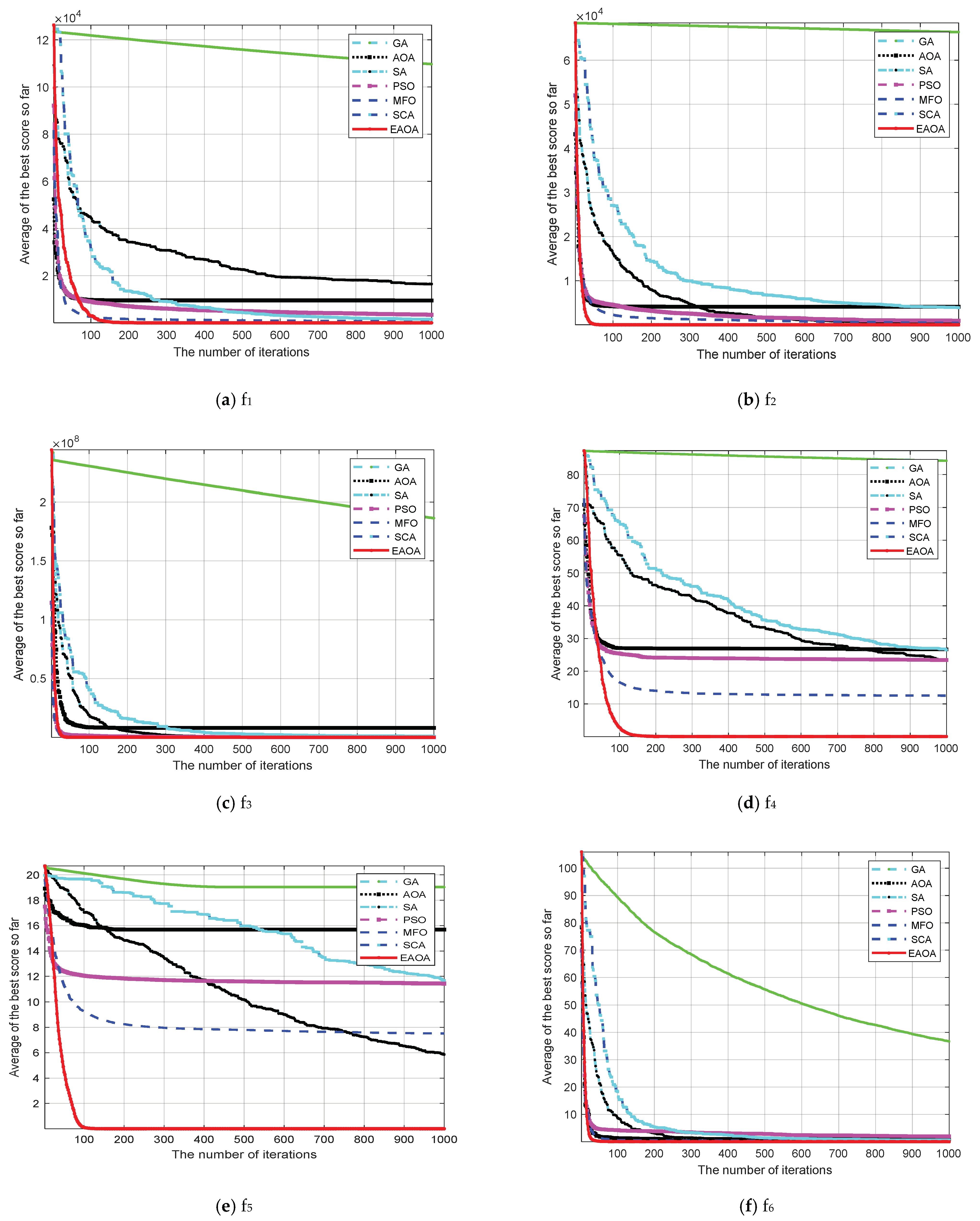
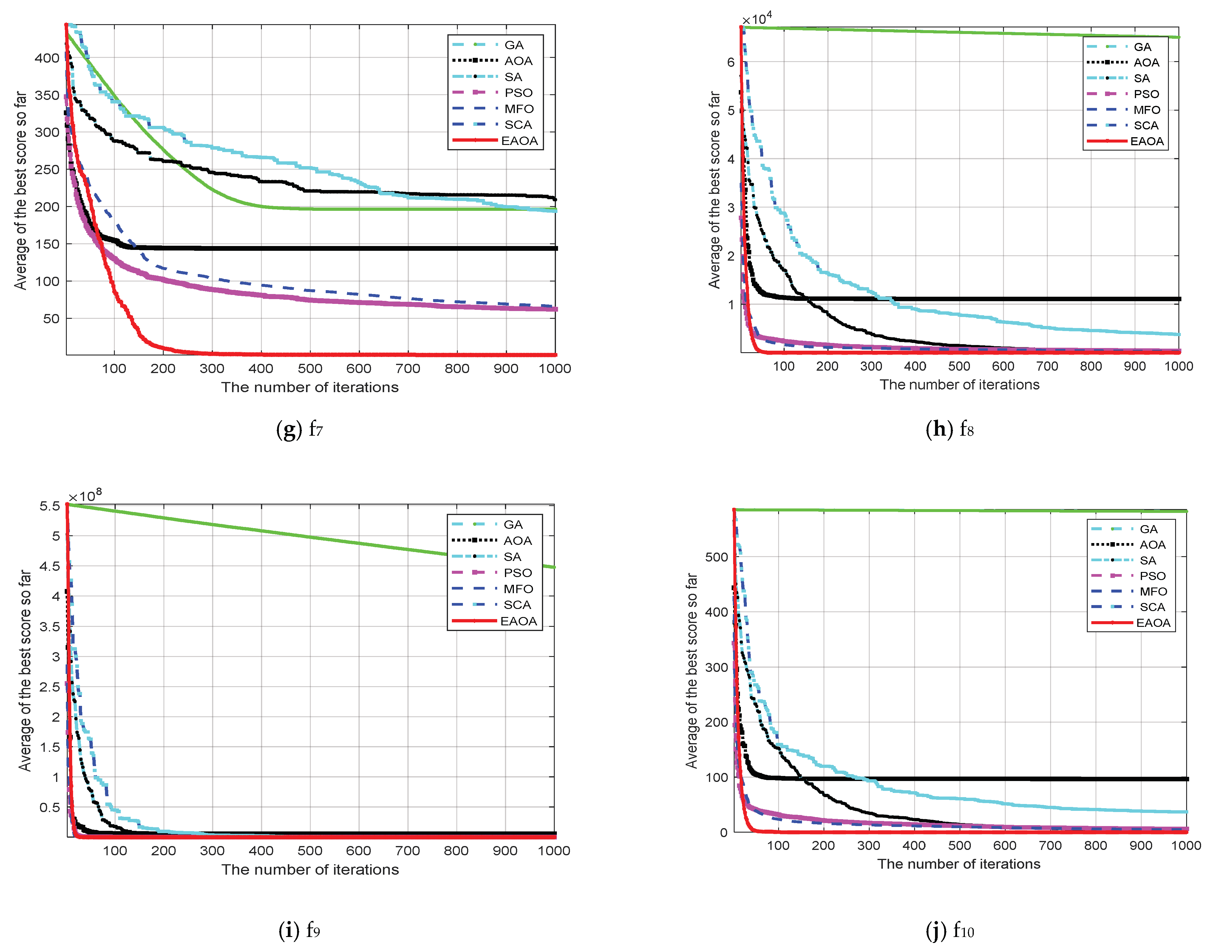
3.2. Experimental Results for Global Optimization
4. Optimal WSN Node Coverage Based on EAOA
4.1. Optimal Node Coverage Strategy
- Step 1: Input parameters such as a number of nodes , perception radius , area of region , etc.
- Step 2: Set the parameters of population size N, the maximum number of iterations max_Iter, the density factor, and prey attraction, and randomly initialize the object’s positions using Equations (5)–(7).
- Step 3: Enhance the initializing population—the parameters of Equations (8)–(10), (14), and (15)—and calculate the objective function for initial coverage according to Equation (18).
- Step 4: Update the position of objects and the strategy according to Equation (17), and then compare them to select the best fitness value according to the objective function value.
- Step 5: Calculate the individual values of objects and retain the optimal solution of the global best.
- Step 6: Determine whether the end condition is reached; if yes, proceed to the next step; otherwise, return to Step 4.
- Step 7: The program ends and outputs the optimal fitness value and the object’s best location, representing the node’s optimal coverage rate outputs.
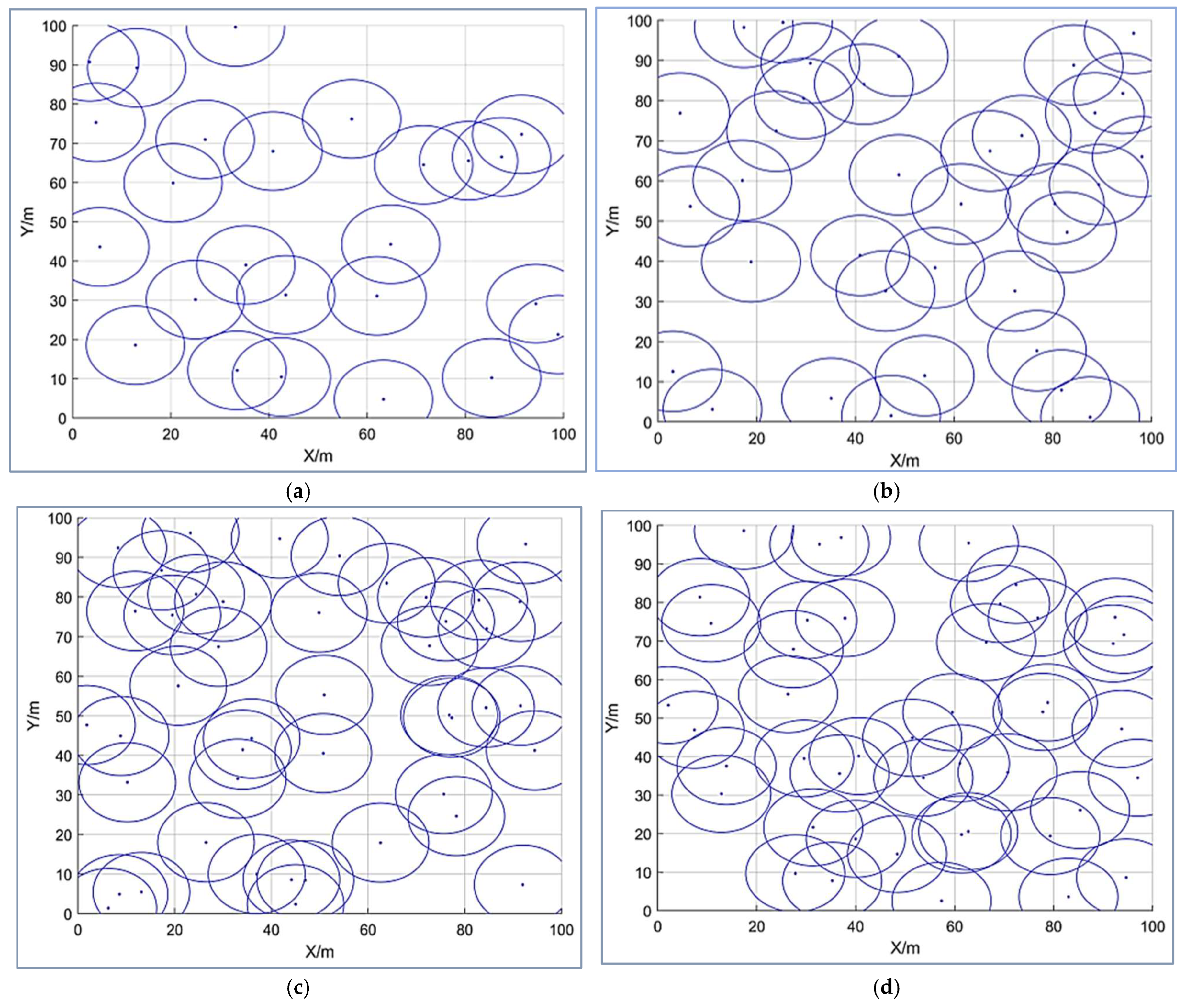
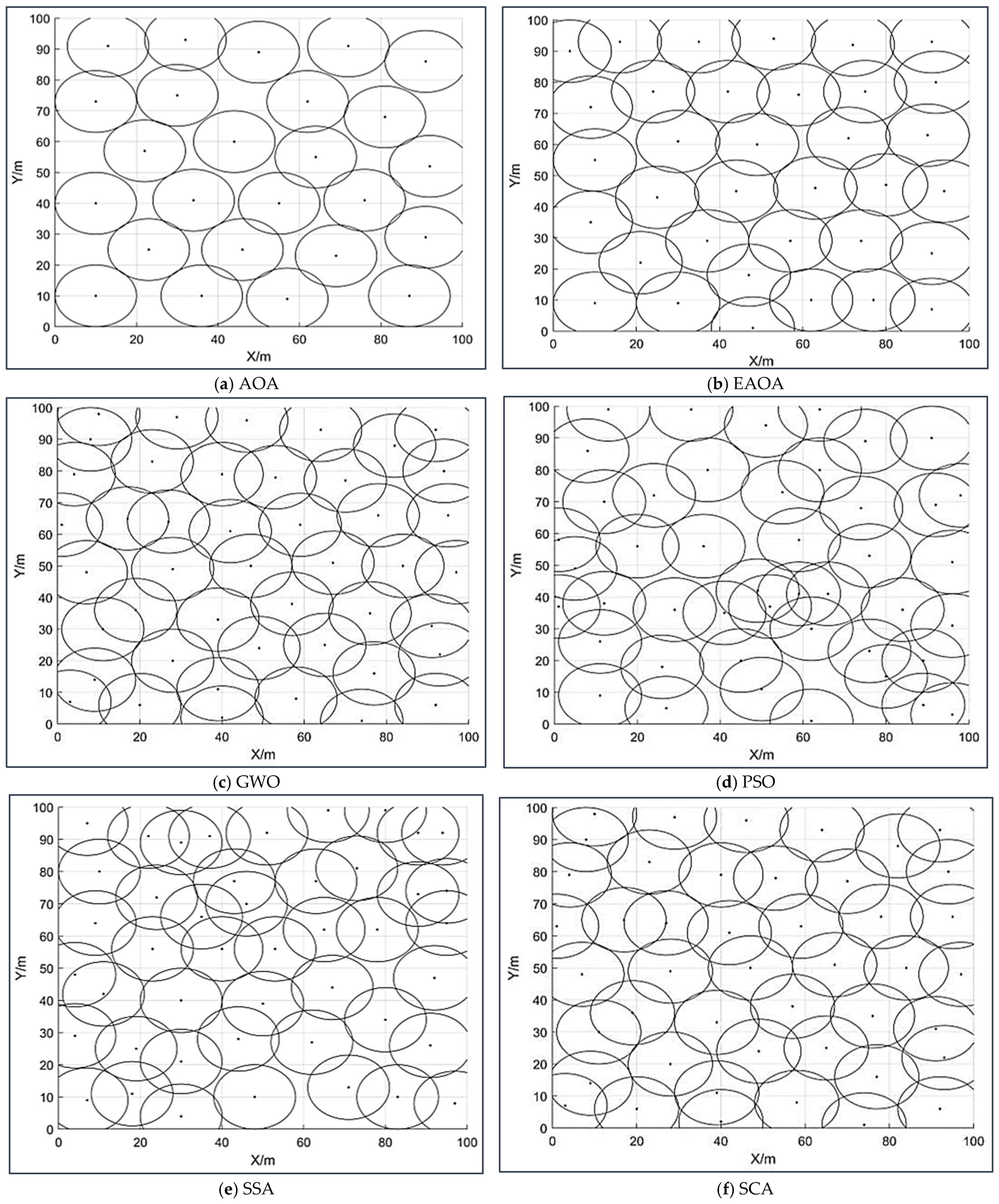
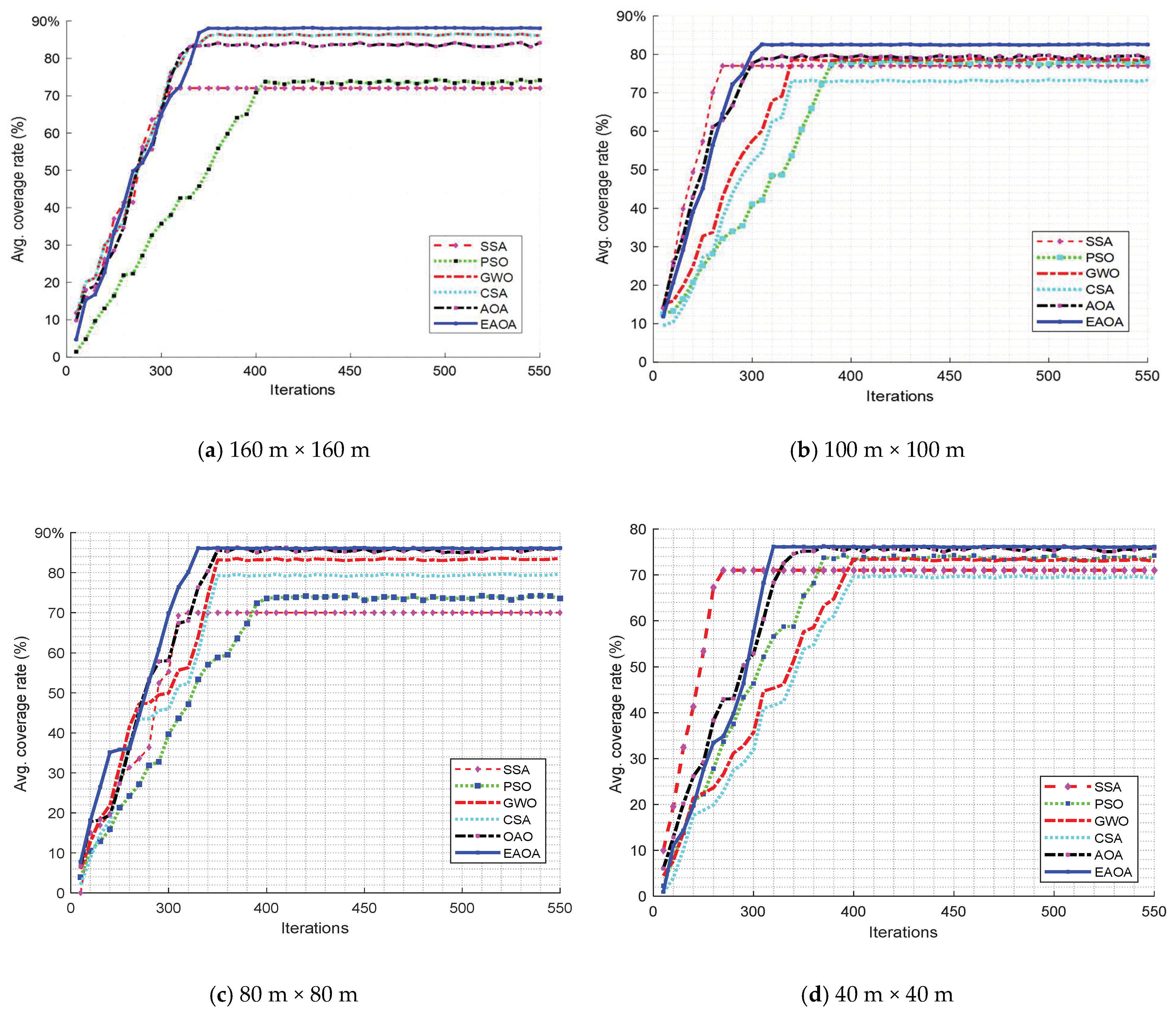
4.2. Analysis and Discussion of Results
5. Conclusions
Author Contributions
Funding
Institutional Review Board Statement
Informed Consent Statement
Data Availability Statement
Conflicts of Interest
Appendix A

| Fun Test | Original | Suggested Strategy 01 | Suggested Strategy 02 | Suggested Strategies 01 and 02 | ||||
|---|---|---|---|---|---|---|---|---|
| AOA | Multidirection | Opposite Learning | EAOA | |||||
| Mean | CPU Runtime (s) | Mean | CPU Runtime (s) | Mean | CPU Runtime (s) | Mean | CPU Runtime (s) | |
| f1 | 2.95 × 10⁻¹ | 37.93 | 1.86 × 10⁻¹ | 36.10 | 1.91 × 10⁻¹ | 34.30 | 1.71 × 10⁻¹ | 38.52 |
| f2 | 2.71 × 10+1 | 32.76 | 1.94 × 10+1 | 34.02 | 1.61 × 10+1 | 34.12 | 1.65 × 10+1 | 38.32 |
| f3 | 3.66 × 10⁻¹ | 45.34 | 2.58 × 10⁻¹ | 47.09 | 6.52 × 10⁻² | 47.23 | 2.44 × 10⁻¹ | 53.04 |
| f4 | 3.02 × 10⁻¹ | 44.16 | 1.45 × 10⁻¹ | 45.86 | 4.59 × 10⁻² | 46.00 | 1.27 × 10⁻² | 52.12 |
| f5 | 7.99 × 10⁻² | 40.32 | 7.84 × 10⁻³ | 42.81 | 1.38 × 10⁻² | 42.00 | 5.38 × 10⁻³ | 48.03 |
| f6 | 5.58 × 10⁻¹ | 85.44 | 2.11 × 10⁻¹ | 88.73 | 6.21 × 10⁻² | 89.00 | 1.92 × 10⁻¹ | 98.89 |
| f7 | 2.21 × 10⁻¹ | 203.52 | 1.07 × 10⁻¹ | 221.31 | 2.44 × 10⁻¹ | 212.10 | 1.26 × 10⁻¹ | 237.18 |
| f8 | 6.32 × 100 | 117.12 | 6.61 × 10⁻¹ | 121.41 | 1.97 × 100 | 122.00 | 7.25 × 10⁻¹ | 136.23 |
| f9 | 7.20 × 100 | 229.60 | 4.82 × 100 | 234.61 | 4.25 × 100 | 235.010 | 4.36 × 100 | 251.72 |
| f10 | 2.25 × 100 | 224.61 | 2.63 × 10⁻¹ | 233.42 | 2.05 × 10⁻¹ | 234.10 | 2.10 × 10⁻² | 263.69 |
| f11 | 4.95 × 10+3 | 274.65 | 1.77 × 10+3 | 275.31 | 8.09 × 10+3 | 278.01 | 1.06 × 10+3 | 278.59 |
| f12 | 1.66 × 10+2 | 229.44 | 3.65 × 10+1 | 238.28 | 8.09 × 10+1 | 239.00 | 2.29 × 10+1 | 268.40 |
| f13 | 3.58 × 10+1 | 120.01 | 2.87 × 100 | 124.61 | 3.30 × 10+1 | 125.10 | 1.53 × 100 | 140.28 |
| f14 | 2.96 × 10+1 | 96.26 | 1.62 × 100 | 100.71 | 1.09 × 10+1 | 101.10 | 1.26 × 100 | 113.41 |
| f15 | 2.05 × 100 | 221.76 | 7.88 × 10⁻¹ | 231.31 | 4.74 × 10⁻¹ | 231.10 | 7.27 × 10⁻¹ | 259.42 |
| f16 | 4.73 × 10⁻¹ | 126.72 | 1.85 × 10⁻¹ | 131.61 | 2.59 × 10⁻¹ | 132.01 | 1.30 × 10⁻¹ | 148.34 |
| f17 | 4.04 × 10+2 | 223.69 | 5.63 × 10+1 | 232.31 | 5.53 × 10+2 | 233.10 | 7.90 × 10+1 | 262.71 |
| f18 | 2.49 × 10+2 | 100.81 | 3.70 × 10⁻¹ | 104.35 | 1.46 × 10+1 | 105.10 | 1.09 × 100 | 117.92 |
| f19 | 4.06 × 10⁻¹ | 206.40 | 3.24 × 10⁻¹ | 214.36 | 3.79 × 10⁻¹ | 215.00 | 3.86 × 10⁻¹ | 241.45 |
| f20 | 5.87 × 10⁻¹ | 298.56 | 4.11 × 10⁻¹ | 310.07 | 4.34 × 10⁻² | 311.00 | 3.98 × 10⁻² | 349.25 |
| f21 | 6.51 × 10⁻¹ | 327.36 | 2.25 × 10⁻¹ | 339.98 | 8.29 × 10⁻² | 341.00 | 2.10 × 10⁻¹ | 384.15 |
| f22 | 8.94 × 10⁻¹ | 312.96 | 6.22 × 10⁻¹ | 325.76 | 7.03 × 10⁻¹ | 326.00 | 6.34 × 10⁻¹ | 367.09 |
| f23 | 1.02 × 10 | 303.36 | 7.63 × 10⁻¹ | 315.05 | 5.72 × 10⁻² | 316.00 | 7.59 × 10⁻² | 354.87 |
| f24 | 7.38 × 10⁻¹ | 282.24 | 6.63 × 10⁻¹ | 294.32 | 4.75 × 10⁻¹ | 294.00 | 4.12 × 10⁻¹ | 331.25 |
| f25 | 3.28 × 100 | 206.40 | 7.26 × 10⁻¹ | 215.36 | 1.51 × 100 | 215.00 | 7.74 × 10⁻¹ | 243.15 |
| f26 | 8.53 × 10⁻¹ | 253.44 | 8.03 × 10⁻¹ | 263.22 | 2.78 × 10⁻² | 264.00 | 7.78 × 10⁻¹ | 297.17 |
| f27 | 7.28 × 10⁻¹ | 273.44 | 7.74 × 10⁻¹ | 265.45 | 5.19 × 10⁻¹ | 284.00 | 7.41 × 10⁻² | 295.92 |
| f28 | 2.37 × 100 | 225.60 | 1.09 × 100 | 234.30 | 3.34 × 10⁻¹ | 235.00 | 9.39 × 10⁻¹ | 263.91 |
| f29 | 2.15 × 10+3 | 221.76 | 8.37 × 10+1 | 230.31 | 3.14 × 10+2 | 231.12 | 4.67 × 10+1 | 259.82 |
| Avg. | 1.72 × 10⁻¹ | 198.01 | 6.88 × 10⁻¹ | 199.91 | 3.15 × 10⁻¹ | 199.47 | 4.45 × 10⁻² | 219.12 |
| Funs | GA | SA | EAOA | ||||||
|---|---|---|---|---|---|---|---|---|---|
| Mean | Best | Std. | Mean | Best | Std. | Mean | Best | Std. | |
| f1 | 5.66 × 10⁻⁵ | 1.46 × 10⁻⁵ | 5.19 × 10⁻⁵ | 7.16 × 10⁻⁵ | 1.25 × 10⁻⁵ | 2.38 × 10⁻⁵ | 1.29 × 10⁻⁵ | 2.71 × 10⁻⁵ | 1.11 × 10⁻⁵ |
| f2 | 3.72 × 10⁻¹ | 1.54 × 10⁻¹ | 1.01 × 10⁻¹ | 3.78 × 10+1 | 2.21 × 10+1 | 9.86 × 10+1 | 3.57 × 10⁻¹ | 1.85 × 10⁻¹ | 1.11 × 10⁻¹ |
| f3 | 2.57 × 10⁻¹ | 1.58 × 10⁻¹ | 5.11 × 10⁻² | 4.92 × 10⁻¹ | 2.66 × 10⁻¹ | 1.28 × 10⁻¹ | 2.33 × 10⁻¹ | 1.44 × 10⁻¹ | 5.52 × 10⁻² |
| f4 | 2.31 × 10⁻¹ | 1.45 × 10⁻¹ | 4.84 × 10⁻² | 4.58 × 10⁻¹ | 3.02 × 10⁻¹ | 4.34 × 10⁻² | 1.91 × 10⁻¹ | 1.11 × 10⁻¹ | 4.59 × 10⁻² |
| f5 | 3.90 × 10⁻² | 7.86 × 10⁻³ | 1.68 × 10⁻² | 1.12 × 10⁻² | 7.99 × 10⁻² | 1.63 × 10⁻² | 2.57 × 10⁻² | 5.38 × 10⁻³ | 1.38 × 10⁻² |
| f6 | 3.28 × 10⁻¹ | 2.11 × 10⁻¹ | 7.81 × 10⁻² | 8.30 × 10⁻¹ | 5.58 × 10⁻¹ | 1.26 × 10⁻¹ | 2.68 × 10⁻¹ | 1.92 × 10⁻¹ | 6.21 × 10⁻² |
| f7 | 1.95 × 10⁻¹ | 1.07 × 10⁻¹ | 3.69 × 10⁻² | 3.59 × 10⁻¹ | 2.21 × 10⁻¹ | 8.33 × 10⁻² | 1.66 × 10⁻¹ | 1.26 × 10⁻¹ | 2.44 × 10⁻² |
| f8 | 3.43 × 100 | 1.21 × 10+1 | 1.64 × 100 | 1.32 × 100 | 6.32 × 100 | 4.29 × 100 | 3.23 × 100 | 7.17 × 10⁻¹ | 1.97 × 100 |
| f9 | 6.43 × 100 | 4.81 × 100 | 1.19 × 100 | 8.79 × 100 | 7.20 × 100 | 1.09 × 100 | 6.53 × 100 | 4.36 × 100 | 1.25 × 100 |
| f10 | 3.99 × 10⁻¹ | 2.03 × 10⁻¹ | 1.03 × 10⁻¹ | 5.33 × 100 | 1.20 × 100 | 4.24 × 100 | 3.81 × 10⁻¹ | 2.10 × 10⁻¹ | 1.01 × 10⁻¹ |
| f11 | 1.02 × 10+4 | 1.77 × 10+3 | 9.36 × 10+3 | 2.81 × 10+5 | 4.45 × 10+4 | 1.90 × 10+5 | 7.58 × 10+3 | 1.06 × 10+3 | 8.09 × 10+3 |
| f12 | 9.53 × 10+2 | 3.65 × 10+1 | 1.07 × 10+2 | 9.30 × 10+2 | 1.66 × 10+2 | 1.10 × 10+3 | 9.47 × 10+1 | 2.29 × 10+1 | 8.09 × 10+1 |
| f13 | 3.62 × 10+1 | 9.87 × 100 | 3.51 × 10+1 | 9.11 × 10+3 | 9.80 × 100 | 2.89 × 10+2 | 9.23 × 10+1 | 9.83 × 100 | 3.30 × 10+1 |
| f14 | 1.21 × 10+1 | 1.62 × 100 | 7.68 × 100 | 1.66 × 10+2 | 2.96 × 10+1 | 1.15 × 10+2 | 1.05 × 10+1 | 1.26 × 100 | 1.09 × 10+1 |
| f15 | 1.57 × 100 | 7.88 × 10⁻¹ | 4.83 × 10⁻¹ | 3.69 × 100 | 2.05 × 100 | 4.63 × 10⁻¹ | 1.66 × 100 | 7.27 × 10⁻¹ | 4.74 × 10⁻¹ |
| f16 | 5.97 × 10⁻¹ | 1.85 × 10⁻¹ | 2.70 × 10⁻¹ | 1.30 × 100 | 4.73 × 10⁻¹ | 3.87 × 10⁻¹ | 5.77 × 10⁻¹ | 1.30 × 10⁻¹ | 2.59 × 10⁻¹ |
| f17 | 6.05 × 10+2 | 5.63 × 10+1 | 7.15 × 10+2 | 1.01 × 10+4 | 4.04 × 10+2 | 1.60 × 10+4 | 4.81 × 10+2 | 7.90 × 10+1 | 5.53 × 10+2 |
| f18 | 9.73 × 100 | 3.70 × 10⁻¹ | 1.74 × 10+1 | 2.11 × 10+4 | 2.49 × 10+2 | 1.87 × 10+4 | 1.10 × 10+1 | 1.09 × 100 | 1.46 × 10+1 |
| f19 | 7.95 × 10⁻¹ | 3.24 × 10⁻¹ | 3.13 × 10⁻¹ | 1.29 × 10⁻¹ | 4.06 × 10⁻¹ | 3.70 × 10⁻¹ | 7.97 × 10⁻¹ | 3.86 × 10⁻¹ | 2.79 × 10⁻¹ |
| f20 | 4.87 × 10⁻¹ | 4.11 × 10⁻¹ | 3.48 × 10⁻² | 7.39 × 10⁻¹ | 5.87 × 10⁻¹ | 8.77 × 10⁻² | 4.80 × 10⁻¹ | 3.98 × 10⁻¹ | 4.34 × 10⁻² |
| f21 | 3.46 × 10⁻¹ | 2.25 × 10⁻¹ | 6.95 × 10⁻² | 8.38 × 100 | 6.51 × 10⁻¹ | 2.32 × 100 | 2.95 × 10⁻¹ | 2.10 × 10⁻¹ | 8.29 × 10⁻² |
| f22 | 7.69 × 10⁻¹ | 6.22 × 10⁻¹ | 5.70 × 10⁻² | 1.21 × 100 | 9.94 × 10⁻¹ | 1.04 × 10⁻¹ | 7.46 × 10⁻¹ | 6.79 × 10⁻¹ | 4.63 × 10⁻² |
| f23 | 8.64 × 10⁻¹ | 7.63 × 10⁻¹ | 6.44 × 10⁻² | 1.26 × 100 | 1.02 × 10⁻¹ | 1.34 × 10⁻¹ | 8.49 × 10⁻¹ | 7.59 × 10⁻¹ | 5.72 × 10⁻² |
| f24 | 7.34 × 10⁻¹ | 6.63 × 10⁻¹ | 3.85 × 10⁻² | 8.77 × 10⁻¹ | 7.38 × 10⁻¹ | 7.48 × 10⁻² | 7.00 × 10⁻¹ | 6.12 × 10⁻¹ | 4.75 × 10⁻² |
| f25 | 2.79 × 100 | 7.26 × 10⁻¹ | 1.62 × 100 | 8.04 × 100 | 3.28 × 100 | 1.63 × 100 | 3.45 × 100 | 7.74 × 10⁻¹ | 1.51 × 100 |
| f26 | 8.44 × 10⁻¹ | 8.03 × 10⁻¹ | 2.31 × 10⁻² | 1.13 × 100 | 8.53 × 10⁻¹ | 1.82 × 10⁻¹ | 8.29 × 10⁻¹ | 7.78 × 10⁻¹ | 2.78 × 10⁻² |
| f27 | 8.55 × 10⁻¹ | 7.74 × 10⁻¹ | 5.76 × 10⁻² | 1.02 × 100 | 8.28 × 10⁻¹ | 1.38 × 10⁻¹ | 8.17 × 10⁻¹ | 7.41 × 10⁻¹ | 5.19 × 10⁻² |
| f28 | 1.74 × 100 | 1.09 × 100 | 3.76 × 10⁻¹ | 3.66 × 100 | 2.37 × 10⁻¹ | 6.31 × 10⁻¹ | 1.49 × 100 | 9.39 × 10⁻¹ | 3.34 × 10⁻¹ |
| f29 | 1.12 × 10+3 | 8.37 × 10+1 | 1.16 × 10+3 | 4.33 × 10+4 | 4.15 × 10+3 | 3.70 × 10+4 | 3.55 × 10+2 | 4.89 × 10+1 | 3.14 × 10+2 |
| Win | 5 | 9 | 7 | 6 | 5 | 5 | 20 | 18 | 19 |
| Lose | 21 | 18 | 20 | 22 | 22 | 22 | 9 | 11 | 10 |
| Draw | 3 | 4 | 4 | 3 | 2 | 4 | 0 | 0 | 0 |
| Funs | FPA | PSO | EAOA | ||||||
|---|---|---|---|---|---|---|---|---|---|
| Mean | Best | Std. | Mean | Best | Std. | Mean | Best | Std. | |
| f1 | 2.24 × 10⁻² | 1.19 × 10⁻² | 5.79 × 10⁻² | 4.37 × 10⁻² | 2.25 × 10⁻² | 1.36 × 10⁻² | 1.34 × 10⁻³ | 2.83 × 10⁻² | 1.16 × 10⁻² |
| f2 | 1.15 × 100 | 7.23 × 10⁻¹ | 2.60 × 10⁻¹ | 8.74 × 10⁻¹ | 5.18 × 10⁻¹ | 6.01 × 10⁻¹ | 7.58 × 10⁻¹ | 3.92 × 10⁻¹ | 4.36 × 10⁻¹ |
| f3 | 2.11 × 10⁻¹ | 1.43 × 10⁻¹ | 3.47 × 10⁻¹ | 2.34 × 10⁻¹ | 1.21 × 10⁻¹ | 3.40 × 10⁻¹ | 2.43 × 10⁻¹ | 1.50 × 10⁻¹ | 5.77 × 10⁻² |
| f4 | 3.45 × 10⁻¹ | 2.40 × 10⁻¹ | 5.46 × 10⁻² | 2.55 × 10⁻¹ | 1.63 × 10⁻¹ | 3.90 × 10⁻² | 2.00 × 10⁻¹ | 1.16 × 10⁻¹ | 4.80 × 10⁻² |
| f5 | 6.68 × 10⁻² | 2.54 × 10⁻² | 1.98 × 10⁻² | 7.62 × 10⁻² | 4.46 × 10⁻² | 1.20 × 10⁻² | 2.68 × 10⁻² | 5.63 × 10⁻³ | 1.44 × 10⁻² |
| f6 | 4.30 × 10⁻¹ | 3.80 × 10⁻¹ | 2.70 × 10⁻² | 3.26 × 10⁻¹ | 2.50 × 10⁻¹ | 4.61 × 10⁻² | 2.81 × 10⁻¹ | 2.01 × 10⁻¹ | 6.49 × 10⁻² |
| f7 | 2.59 × 10⁻¹ | 1.96 × 10⁻¹ | 3.70 × 10⁻² | 1.98 × 10⁻¹ | 1.36 × 10⁻¹ | 2.82 × 10⁻² | 1.73 × 10⁻¹ | 1.32 × 10⁻¹ | 1.25 × 10⁻¹ |
| f8 | 4.69 × 100 | 1.11 × 10⁻¹ | 2.95 × 100 | 4.42 × 100 | 1.83 × 100 | 1.59 × 100 | 3.37 × 100 | 7.49 × 10⁻¹ | 2.06 × 100 |
| f9 | 9.68 × 100 | 7.43 × 100 | 1.17 × 100 | 7.17 × 100 | 4.82 × 100 | 5.09 × 100 | 6.82 × 100 | 4.56 × 100 | 1.30 × 100 |
| f10 | 4.07 × 10⁻¹ | 2.77 × 10⁻¹ | 6.08 × 10⁻² | 3.14 × 10⁻¹ | 2.25 × 10⁻¹ | 4.61 × 10⁻² | 3.98 × 10⁻¹ | 2.19 × 10⁻¹ | 1.06 × 10⁻¹ |
| f11 | 3.01 × 10+1 | 3.25 × 10+1 | 3.26 × 10+1 | 3.13 × 10+1 | 3.15 × 10+1 | 3.15 × 10+1 | 3.40 × 10+1 | 3.11 × 10+1 | 3.10 × 10+1 |
| f12 | 7.20 × 10+2 | 3.72 × 10+2 | 8.30 × 10+2 | 1.11 × 10+2 | 4.52 × 10+1 | 4.62 × 10+1 | 9.90 × 10+1 | 2.39 × 10+1 | 8.46 × 10+1 |
| f13 | 7.34 × 10+1 | 8.89 × 100 | 6.28 × 10+1 | 2.59 × 10+1 | 5.45 × 10⁻¹ | 2.66 × 10+1 | 3.06 × 10+1 | 1.59 × 100 | 3.44 × 10+1 |
| f14 | 3.03 × 10+2 | 8.32 × 10+1 | 2.17 × 10+2 | 4.57 × 10+1 | 1.92 × 10+1 | 2.71 × 10+1 | 1.10 × 10+1 | 1.32 × 100 | 1.14 × 10+1 |
| f15 | 2.01 × 100 | 1.09 × 100 | 3.70 × 10⁻¹ | 2.01 × 100 | 1.26 × 100 | 4.51 × 10⁻¹ | 1.73 × 100 | 7.59 × 10⁻¹ | 4.95 × 10⁻¹ |
| f16 | 7.50 × 10⁻¹ | 2.41 × 10⁻¹ | 2.38 × 10⁻¹ | 6.40 × 10⁻¹ | 1.93 × 10⁻¹ | 2.80 × 10⁻¹ | 6.03 × 10⁻¹ | 1.36 × 10⁻¹ | 2.70 × 10⁻¹ |
| f17 | 9.05 × 10+1 | 5.47 × 10+1 | 1.23 × 10+2 | 9.08 × 10+1 | 1.09 × 10+1 | 8.55 × 10+1 | 1.02 × 10+2 | 1.68 × 10+1 | 1.17 × 10+2 |
| f18 | 1.50 × 10+2 | 4.30 × 10+1 | 1.32 × 10+2 | 2.42 × 10+1 | 1.64 × 100 | 2.35 × 10+1 | 1.38 × 100 | 1.37 × 10⁻¹ | 1.84 × 100 |
| f19 | 7.85 × 10⁻¹ | 4.36 × 10⁻¹ | 2.39 × 10⁻¹ | 7.69 × 10⁻¹ | 5.01 × 10⁻¹ | 1.78 × 10⁻¹ | 8.33 × 10⁻¹ | 4.03 × 10⁻¹ | 2.91 × 10⁻¹ |
| f20 | 6.30 × 10⁻¹ | 5.39 × 10⁻¹ | 4.59 × 10⁻² | 5.71 × 10⁻¹ | 4.96 × 10⁻¹ | 4.14 × 10⁻² | 5.02 × 10⁻¹ | 4.16 × 10⁻¹ | 4.53 × 10⁻² |
| f21 | 1.45 × 100 | 2.33 × 10⁻¹ | 3.18 × 100 | 7.42 × 10⁻¹ | 2.04 × 10⁻¹ | 2.02 × 100 | 3.08 × 10⁻¹ | 2.20 × 10⁻¹ | 8.66 × 10⁻² |
| f22 | 1.03 × 100 | 7.09 × 10⁻¹ | 9.12 × 10⁻¹ | 9.97 × 10⁻¹ | 8.73 × 10⁻¹ | 9.76 × 10⁻¹ | 7.80 × 10⁻¹ | 7.10 × 10⁻¹ | 4.83 × 10⁻² |
| f23 | 1.09 × 100 | 9.27 × 10⁻¹ | 7.47 × 10⁻² | 1.05 × 100 | 8.69 × 10⁻¹ | 8.62 × 10⁻² | 8.87 × 10⁻¹ | 7.93 × 10⁻¹ | 5.98 × 10⁻² |
| f24 | 7.17 × 10⁻¹ | 6.52 × 10⁻¹ | 3.44 × 10⁻² | 7.17 × 10⁻¹ | 6.61 × 10⁻¹ | 3.69 × 10⁻² | 7.32 × 10⁻¹ | 6.39 × 10⁻¹ | 4.96 × 10⁻² |
| f25 | 3.91 × 100 | 6.47 × 10⁻¹ | 2.82 × 100 | 3.26 × 100 | 5.36 × 10⁻¹ | 2.80 × 100 | 3.60 × 100 | 8.08 × 10⁻¹ | 1.57 × 100 |
| f26 | 9.56 × 10⁻¹ | 8.58 × 10⁻¹ | 8.74 × 10⁻² | 9.93 × 10⁻¹ | 8.44 × 10⁻¹ | 7.07 × 10⁻² | 8.66 × 10⁻¹ | 8.12 × 10⁻¹ | 2.90 × 10⁻² |
| f27 | 7.98 × 10⁻¹ | 7.24 × 10⁻¹ | 3.70 × 10⁻² | 7.86 × 10⁻¹ | 6.96 × 10⁻¹ | 4.20 × 10⁻² | 8.54 × 10⁻¹ | 7.74 × 10⁻¹ | 5.43 × 10⁻² |
| f28 | 2.03 × 100 | 1.31 × 100 | 4.27 × 10⁻¹ | 2.38 × 100 | 1.47 × 100 | 4.32 × 10⁻¹ | 1.56 × 100 | 9.81 × 10⁻¹ | 3.49 × 10⁻¹ |
| f29 | 5.47 × 10+3 | 1.89 × 10+3 | 2.54 × 10+3 | 2.89 × 10+3 | 4.93 × 10+2 | 1.89 × 10+3 | 3.71 × 10+2 | 1.01 × 10+2 | 3.28 × 10+2 |
| Win | 5 | 5 | 6 | 7 | 7 | 10 | 18 | 18 | 13 |
| Lose | 23 | 23 | 21 | 21 | 21 | 12 | 11 | 10 | 16 |
| Draw | 3 | 3 | 2 | 1 | 1 | 1 | 0 | 1 | 0 |
| Funs | MFO | SCA | EAOA | ||||||
|---|---|---|---|---|---|---|---|---|---|
| Mean | Best | Std. | Mean | Best | Std. | Mean | Best | Std. | |
| f1 | 4.60 × 10⁻¹ | 2.99 × 10⁻¹ | 7.04 × 10⁻¹ | 2.41 × 10⁻¹ | 1.23 × 10⁻¹ | 4.80 × 10⁻¹ | 1.34 × 10⁻¹ | 2.83 × 10⁻¹ | 1.16 × 10⁻¹ |
| f2 | 2.33 × 10+2 | 9.80 × 10+1 | 1.30 × 10+2 | 1.41 × 10+1 | 9.03 × 10+1 | 2.65 × 10+1 | 3.73 × 10+1 | 1.93 × 10+1 | 1.16 × 10+1 |
| f3 | 6.57 × 100 | 4.83 × 100 | 1.17 × 100 | 2.97 × 10⁻¹ | 1.36 × 10⁻¹ | 8.95 × 10⁻¹ | 2.43 × 10⁻¹ | 1.50 × 10⁻¹ | 5.77 × 10⁻² |
| f4 | 6.23 × 10⁻¹ | 5.46 × 10⁻¹ | 4.52 × 10⁻² | 5.24 × 10⁻¹ | 4.54 × 10⁻¹ | 3.69 × 10⁻² | 2.00 × 10⁻¹ | 1.16 × 10⁻¹ | 4.80 × 10⁻² |
| f5 | 1.38 × 10⁻¹ | 1.21 × 10⁻¹ | 1.43 × 10⁻² | 6.61 × 10⁻² | 6.50 × 10⁻² | 1.54 × 10⁻² | 6.68 × 10⁻² | 5.63 × 10⁻³ | 1.44 × 10⁻² |
| f6 | 1.79 × 100 | 1.34 × 10⁻¹ | 1.66 × 100 | 9.48 × 10⁻¹ | 7.89 × 10⁻¹ | 9.52 × 10⁻² | 2.81 × 10⁻¹ | 2.01 × 10⁻¹ | 6.49 × 10⁻² |
| f7 | 5.83 × 10⁻¹ | 5.16 × 10⁻¹ | 2.83 × 10⁻² | 4.86 × 10⁻¹ | 3.81 × 10⁻¹ | 2.13 × 10⁻² | 1.73 × 10⁻¹ | 1.32 × 10⁻¹ | 2.54 × 10⁻² |
| f8 | 2.38 × 10⁻¹ | 1.78 × 100 | 3.28 × 100 | 1.17 × 10+1 | 5.84 × 100 | 3.05 × 100 | 3.37 × 100 | 7.49 × 10⁻¹ | 2.06 × 100 |
| f9 | 9.99 × 100 | 9.31 × 100 | 3.36 × 10⁻¹ | 1.23 × 10+1 | 1.05 × 10+1 | 6.06 × 10⁻¹ | 6.82 × 100 | 4.56 × 100 | 1.30 × 100 |
| f10 | 7.53 × 100 | 3.80 × 100 | 1.73 × 100 | 3.00 × 10⁻¹ | 1.14 × 10⁻¹ | 9.63 × 10⁻¹ | 3.98 × 10⁻¹ | 2.19 × 10⁻¹ | 1.06 × 10⁻¹ |
| f11 | 2.90 × 10+6 | 1.62 × 10+6 | 5.79 × 10+5 | 1.78 × 10+6 | 9.66 × 10+5 | 5.17 × 10+5 | 7.92 × 10+5 | 1.10 × 10+5 | 8.45 × 10+5 |
| f12 | 7.12 × 10+5 | 3.18 × 10+5 | 2.50 × 10+5 | 3.12 × 10+5 | 8.18 × 10+4 | 2.17 × 10+5 | 9.90 × 10+4 | 8.39 × 10+4 | 8.46 × 10+4 |
| f13 | 2.14 × 10+2 | 2.04 × 10+1 | 9.37 × 10+1 | 7.63 × 10+2 | 2.93 × 10+1 | 5.99 × 10+2 | 3.06 × 10+1 | 2.59 × 10+1 | 3.44 × 10+1 |
| f14 | 1.93 × 10+4 | 1.54 × 10+3 | 9.89 × 10+3 | 7.40 × 10+3 | 9.60 × 10+2 | 4.59 × 10+3 | 1.10 × 10+1 | 1.32 × 100 | 1.14 × 10+1 |
| f15 | 3.58 × 100 | 3.14 × 10⁻¹ | 2.28 × 100 | 3.76 × 10⁻¹ | 2.59 × 100 | 4.23 × 100 | 1.73 × 100 | 7.59 × 10⁻¹ | 4.95 × 10⁻¹ |
| f16 | 1.42 × 100 | 1.09 × 100 | 1.39 × 10⁻¹ | 1.43 × 100 | 6.64 × 10⁻¹ | 3.42 × 10⁻¹ | 6.03 × 10⁻¹ | 1.36 × 10⁻¹ | 2.70 × 10⁻¹ |
| f17 | 3.40 × 10+2 | 8.93 × 10+2 | 1.31 × 10+3 | 9.63 × 10+3 | 1.88 × 10+3 | 7.49 × 10+3 | 5.03 × 10+2 | 8.25 × 10+1 | 5.78 × 10+2 |
| f18 | 5.66 × 10+4 | 2.32 × 10+4 | 2.43 × 10+4 | 1.32 × 10+4 | 3.22 × 10+3 | 7.60 × 10+3 | 1.15 × 10+1 | 1.14 × 100 | 1.53 × 10+1 |
| f19 | 1.17 × 100 | 9.15 × 10⁻¹ | 1.15 × 10⁻¹ | 1.17 × 100 | 6.21 × 10⁻¹ | 2.66 × 10⁻¹ | 8.33 × 10⁻¹ | 4.03 × 10⁻¹ | 2.91 × 10⁻¹ |
| f20 | 8.92 × 10⁻² | 8.28 × 10⁻² | 9.98 × 10⁻¹ | 8.06 × 10⁻¹ | 7.10 × 10⁻¹ | 4.72 × 10⁻² | 5.02 × 10⁻¹ | 4.16 × 10⁻² | 4.53 × 10⁻² |
| f21 | 9.34 × 100 | 7.19 × 100 | 1.04 × 100 | 3.19 × 100 | 1.95 × 10⁻¹ | 5.98 × 10⁻¹ | 3.08 × 10⁻¹ | 2.20 × 10⁻¹ | 8.66 × 10⁻² |
| f22 | 1.28 × 100 | 1.22 × 10⁻¹ | 4.01 × 10⁻¹ | 1.14 × 100 | 1.05 × 100 | 4.84 × 10⁻² | 7.80 × 10⁻¹ | 7.10 × 10⁻¹ | 4.83 × 10⁻¹ |
| f23 | 1.38 × 100 | 1.27 × 100 | 6.06 × 10⁻² | 1.26 × 100 | 1.13 × 100 | 5.20 × 10⁻² | 8.87 × 10⁻¹ | 7.93 × 10⁻¹ | 5.98 × 10⁻² |
| f24 | 3.78 × 100 | 2.27 × 100 | 5.41 × 10⁻¹ | 1.72 × 10⁻¹ | 1.28 × 10⁻¹ | 2.58 × 10⁻¹ | 7.32 × 10⁻¹ | 6.39 × 10⁻² | 4.96 × 10⁻¹ |
| f25 | 8.23 × 100 | 5.94 × 100 | 9.24 × 10⁻¹ | 6.57 × 100 | 3.22 × 100 | 1.84 × 100 | 3.60 × 100 | 8.08 × 10⁻¹ | 1.57 × 100 |
| f26 | 1.20 × 100 | 1.13 × 100 | 3.57 × 10⁻¹ | 1.20 × 10⁻¹ | 8.15 × 10⁻¹ | 1.74 × 10⁻¹ | 8.66 × 10⁻¹ | 8.12 × 10⁻² | 2.90 × 10⁻¹ |
| f27 | 3.39 × 100 | 2.15 × 10⁻¹ | 6.11 × 10⁻¹ | 2.06 × 100 | 4.31 × 10⁻¹ | 8.16 × 10⁻¹ | 8.54 × 10⁻¹ | 7.74 × 10⁻¹ | 5.43 × 10⁻¹ |
| f28 | 3.20 × 100 | 2.76 × 100 | 2.16 × 10⁻¹ | 3.17 × 100 | 1.92 × 100 | 4.95 × 10⁻¹ | 1.56 × 100 | 9.81 × 10⁻¹ | 3.49 × 10⁻¹ |
| f29 | 8.17 × 10+4 | 5.16 × 10+4 | 2.12 × 10+4 | 4.90 × 10+4 | 1.70 × 10+4 | 2.05 × 10+4 | 3.71 × 10+2 | 1.51 × 10+2 | 3.28 × 10+2 |
| Win | 4 | 5 | 6 | 7 | 6 | 6 | 21 | 20 | 17 |
| Lose | 23 | 21 | 21 | 21 | 22 | 23 | 8 | 9 | 14 |
| Draw | 2 | 3 | 2 | 1 | 1 | 0 | 0 | 0 | 0 |
| Funs | PBA [33] | WOA [36] | PPSO [29] | AOA [41] | IFMO [35] | ESCA [40] | EAOA-Itself |
|---|---|---|---|---|---|---|---|
| f1 | 2.4018 × 10⁻⁷ | 1.4018 × 10⁻¹¹ | 1.7018 × 10⁻¹¹ | 1.1205 × 10⁻⁵ | 6.9641 × 10⁻⁸ | 2.5668 × 10⁻⁷ | ~N/A |
| f2 | 1.4018 × 10⁻¹¹ | 1.4018 × 10⁻¹¹ | 1.4018 × 10⁻¹¹ | 2.2080 × 10⁻⁷ | 7.1665 × 10⁻³ | 1.3749 × 10⁻² | ~N/A |
| f3 | 1.4018 × 10⁻¹¹ | 1.4018 × 10⁻¹¹ | 8.5710 × 10⁻¹¹ | 1.8717 × 10⁻² | 1.8717 × 10⁻² | 4.6578 × 10⁻³ | ~N/A |
| f4 | 1.4018 × 10⁻¹¹ | 1.4018 × 10⁻¹¹ | 1.4018 × 10⁻¹¹ | 4.8753 × 10⁻¹¹ | 1.5456 × 10⁻² | 2.7237 × 10⁻⁵ | ~N/A |
| f5 | 1.4018 × 10⁻¹¹ | 1.5447 × 10⁻¹¹ | 1.4018 × 10⁻¹¹ | 1.8376 × 10⁻⁹ | 5.3326 × 10⁻⁵ | 4.0332 × 10⁻¹¹ | ~N/A |
| f6 | 1.4018 × 10⁻¹¹ | 1.4018 × 10⁻¹¹ | 1.4018 × 10⁻¹¹ | 4.4659 × 10⁻¹⁰ | 6.5678 × 10⁻⁴ | 9.8637 × 10⁻⁴ | ~N/A |
| f7 | 1.4018 × 10⁻¹¹ | 1.4018 × 10⁻¹¹ | 1.7018 × 10⁻¹¹ | 9.4096 × 10⁻¹¹ | 1.6922 × 10⁻³ | 6.2370 × 10⁻⁴ | ~N/A |
| f8 | 1.4018 × 10⁻¹¹ | 3.6674 × 10⁻¹¹ | 1.8745 × 10⁻¹¹ | 8.0856 × 10⁻² | 1.0244 × 10⁻¹ | 1.2706 × 10⁻² | ~N/A |
| f9 | 4.8753 × 10⁻¹¹ | 1.4018 × 10⁻¹¹ | 1.2873 × 10⁻⁸ | 2.0041 × 10⁻⁹ | 3.9045 × 10⁻¹ | 2.6004 × 10⁻¹ | ~N/A |
| f10 | 1.4018 × 10⁻¹¹ | 1.4018 × 10⁻¹¹ | 1.4018 × 10⁻¹¹ | 5.8296 × 10⁻¹ | 9.7754 × 10⁻¹ | 1.5366 × 10⁻³ | ~N/A |
| f11 | 1.4018 × 10⁻¹¹ | 1.4018 × 10⁻¹¹ | 1.4018 × 10⁻¹¹ | 1.5439 × 10⁻⁹ | 1.4703 × 10⁻¹ | 3.1620 × 10⁻⁶ | ~N/A |
| f12 | 1.4018 × 10⁻¹¹ | 1.4018 × 10⁻¹¹ | 6.4699 × 10⁻¹¹ | 1.5447 × 10⁻¹¹ | 1.3749 × 10⁻² | 4.1212 × 10⁻² | ~N/A |
| f13 | 7.1071 × 10⁻¹¹ | 7.8055 × 10⁻¹¹ | 7.1071 × 10⁻¹¹ | 1.2847 × 10⁻⁴ | 8.7693 × 10⁻¹ | 8.2178 × 10⁻¹ | ~N/A |
| f14 | 1.4018 × 10⁻¹¹ | 1.4018 × 10⁻¹¹ | 2.5021 × 10⁻¹¹ | 1.4018 × 10⁻¹¹ | 3.7194 × 10⁻² | 3.6588 × 10⁻⁹ | ~N/A |
| f15 | 1.4018 × 10⁻¹¹ | 1.4018 × 10⁻¹¹ | 4.0332 × 10⁻¹¹ | 2.9096 × 10⁻² | 7.2487 × 10⁻¹ | 7.3779 × 10⁻² | ~N/A |
| f16 | 1.4018 × 10⁻¹¹ | 3.7291 × 10⁻¹⁰ | 6.1854 × 10⁻¹ | 2.7082 × 10⁻² | 7.3779 × 10⁻² | 6.3217 × 10⁻¹ | ~N/A |
| f17 | 7.1071 × 10⁻¹¹ | 1.8745 × 10⁻¹¹ | 1.6408 × 10⁻¹⁰ | 1.4729 × 10⁻⁶ | 9.8877 × 10⁻¹ | 7.2487 × 10⁻¹ | ~N/A |
| f18 | 1.4018 × 10⁻¹¹ | 1.4018 × 10⁻¹¹ | 1.4018 × 10⁻¹¹ | 1.4018 × 10⁻¹¹ | 6.1228 × 10⁻¹ | 6.4699 × 10⁻¹¹ | ~N/A |
| f19 | 2.7567 × 10⁻⁶ | 5.3326 × 10⁻⁵ | 1.8183 × 10⁻⁶ | 4.8148 × 10⁻¹ | 8.9917 × 10⁻¹ | 4.6412 × 10⁻¹ | ~N/A |
| f20 | 1.4018 × 10⁻¹¹ | 1.4018 × 10⁻¹¹ | 1.8745 × 10⁻¹¹ | 1.0328 × 10⁻¹⁰ | 2.5189 × 10⁻² | 4.3218 × 10⁻⁷ | ~N/A |
| f21 | 1.4018 × 10⁻¹¹ | 1.4018 × 10⁻¹¹ | 1.4018 × 10⁻¹¹ | 3.3134 × 10⁻¹ | 7.4745 × 10⁻³ | 6.9641 × 10⁻⁸ | ~N/A |
| f22 | 1.4018 × 10⁻¹¹ | 1.4018 × 10⁻¹¹ | 1.4018 × 10⁻¹¹ | 2.7539 × 10⁻¹¹ | 3.7194 × 10⁻² | 2.5021 × 10⁻¹¹ | ~N/A |
| f23 | 1.4018 × 10⁻¹¹ | 1.4018 × 10⁻¹¹ | 1.4018 × 10⁻¹¹ | 9.4096 × 10⁻¹¹ | 2.2599 × 10⁻¹ | 2.5970 × 10⁻⁹ | ~N/A |
| f24 | 1.4018 × 10⁻¹¹ | 1.4018 × 10⁻¹¹ | 7.8055 × 10⁻¹¹ | 2.0014 × 10⁻¹ | 1.8717 × 10⁻² | 1.7206 × 10⁻¹ | ~N/A |
| f25 | 2.2729 × 10⁻¹¹ | 1.3989 × 10⁻⁷ | 1.3643 × 10⁻¹⁰ | 4.4711 × 10⁻¹ | 8.2178 × 10⁻¹ | 3.1751 × 10⁻¹ | ~N/A |
| f26 | 1.4018 × 10⁻¹¹ | 3.9843 × 10⁻⁹ | 3.0304 × 10⁻¹¹ | 1.1106 × 10⁻⁷ | 2.8074 × 10⁻² | 2.3679 × 10⁻¹⁰ | ~N/A |
| f27 | 1.4018 × 10⁻¹¹ | 9.4096 × 10⁻¹¹ | 5.8443 × 10⁻¹⁰ | 2.1213 × 10⁻⁵ | 5.9218 × 10⁻⁴ | 2.2408 × 10⁻⁶ | ~N/A |
| f28 | 1.4018 × 10⁻¹¹ | 2.2729 × 10⁻¹¹ | 1.4018 × 10⁻¹¹ | 7.1825 × 10⁻⁵ | 2.0181 × 10⁻² | 4.3379 × 10⁻⁹ | ~N/A |
| f29 | 1.4018 × 10⁻¹¹ | 1.4018 × 10⁻¹¹ | 1.4018 × 10⁻¹¹ | 1.4018 × 10⁻¹¹ | 6.2370 × 10⁻⁴ | 7.8055 × 10⁻¹¹ | ~N/A |
| Avg. | 6.5517 | 5.7241 | 5.6207 | 3.6207 | 2.5138 | 2.5483 | 2.25204 |
| Rank | 7 | 6 | 5 | 4 | 2 | 3 | 1 |
Appendix B
References
- Yick, J.; Mukherjee, B.; Ghosal, D. Wireless sensor network survey. Comput. Netw. 2008, 52, 2292–2330. [Google Scholar] [CrossRef]
- Qiao, Y.; Dao, T.K.; Pan, J.S.; Chu, S.C.; Nguyen, T.T. Diversity teams in soccer league competition algorithm for wireless sensor network deployment problem. Symmetry 2020, 12, 445. [Google Scholar] [CrossRef] [Green Version]
- Dao, T.K.; Yu, J.; Nguyen, T.T.; Ngo, T.G. A Hybrid Improved MVO and FNN for Identifying Collected Data Failure in Cluster Heads in WSN. IEEE Access 2020, 8, 124311–124322. [Google Scholar] [CrossRef]
- Dao, T.K.; Nguyen, T.T.; Pan, J.S.; Qiao, Y.; Lai, Q. Identification Failure Data for Cluster Heads Aggregation in WSN Based on Improving Classification of SVM. IEEE Access 2020, 8, 61070–61084. [Google Scholar] [CrossRef]
- Ali, A.; Ming, Y.; Chakraborty, S.; Iram, S. A comprehensive survey on real-time applications of WSN. Future internet 2017, 9, 77. [Google Scholar] [CrossRef] [Green Version]
- Chu, S.C.; Dao, T.K.; Pan, J.S.; Nguyen, T.T. Identifying correctness data scheme for aggregating data in cluster heads of wireless sensor network based on naive Bayes classification. Eurasip J. Wirel. Commun. Netw. 2020, 52. [Google Scholar] [CrossRef] [Green Version]
- Nguyen, T.T.; Pan, J.S.; Dao, T.K. An Improved Flower Pollination Algorithm for Optimizing Layouts of Nodes in Wireless Sensor Network. IEEE Access 2019, 7, 75985–75998. [Google Scholar] [CrossRef]
- Chai, Q.-W.; Chu, S.-C.; Pan, J.-S.; Zheng, W.-M. Applying Adaptive and Self Assessment Fish Migration Optimization on Localization of Wireless Sensor Network on 3-D Terrain. J. Inf. Hiding Multim. Signal Process. 2020, 11, 90–102. [Google Scholar]
- Kulkarni, R.V.R.; Ferster, A.; Venayagamoorthy, G.K. Computational intelligence in wireless sensor networks: A survey. IEEE Commun. Surv. Tutor. 2011, 13, 68–96. [Google Scholar] [CrossRef]
- Li, Z.; Chu, S.-C.; Pan, J.-S.; Hu, P.; Xue, X. A Mahalanobis Surrogate-Assisted Ant Lion Optimization and Its Application in 3D Coverage of Wireless Sensor Networks. Entropy 2022, 24, 586. [Google Scholar] [CrossRef]
- Pan, J.-S.; Dao, T.-K.; Pan, T.-S.; Nguyen, T.-T.; Chu, S.-C.; Roddick, J.F. An improvement of flower pollination algorithm for node localization optimization in WSN. J. Inf. Hiding Multimed. Signal. Process. 2017, 8, 486–499. [Google Scholar]
- Pan, J.-S.; Sun, X.-X.; Chu, S.-C.; Abraham, A.; Yan, B. Digital watermarking with improved SMS applied for QR code. Eng. Appl. Artif. Intell. 2021, 97, 104049. [Google Scholar] [CrossRef]
- Nguyen, T.-T.; Pan, J.-S.; Dao, T.-K.; Sung, T.-W.; Ngo, T.-G. Pigeon-Inspired Optimization for Node Location in Wireless Sensor Network. In Proceedings of the International Conference on Engineering Research and Applications, Thai Nguyen, Vietnam, 1–2 December 2019; Volume 104, pp. 589–598. [Google Scholar]
- Nguyen, T.-T.; Dao, T.-K.; Kao, H.-Y.; Horng, M.-F.; Shieh, C.-S. Hybrid Particle Swarm Optimization with Artificial Bee Colony Optimization for Topology Control Scheme in Wireless Sensor Networks. J. Internet Technol. 2017, 18, 743–752. [Google Scholar] [CrossRef]
- Nguyen, T.-T.; Pan, J.-S.; Wu, T.-Y.; Dao, T.-K.; Nguyen, T.-D. Node Coverage Optimization Strategy Based on Ions Motion Optimization. J. Netw. Intell. 2019, 4, 2414–8105. [Google Scholar]
- Pan, J.-S.; Nguyen, T.-T.; Dao, T.-K.; Pan, T.-S.; Chu, S.-C. Clustering Formation in Wireless Sensor Networks: A Survey. J. Netw. Intell. 2017, 2, 287–309. [Google Scholar]
- Dao, T.K.; Pan, T.S.; Nguyen, T.T.; Chu, S.C. A compact Articial bee colony optimization for topology control scheme in wireless sensor networks. J. Inf. Hiding Multimed. Signal Processing 2015, 6, 297–310. [Google Scholar]
- Othman, M.F.; Shazali, K. Wireless sensor network applications: A study in environment monitoring system. Procedia Eng. 2012, 41, 1204–1210. [Google Scholar] [CrossRef] [Green Version]
- Liu, N.; Pan, J.S.; Nguyen, T.T. A bi-Population QUasi-Affine TRansformation Evolution algorithm for global optimization and its application to dynamic deployment in wireless sensor networks. Eurasip J. Wirel. Commun. Netw. 2019, 2019, 175. [Google Scholar] [CrossRef]
- Mahdavi, S.; Shiri, M.E.; Rahnamayan, S. Metaheuristics in large-Scale global continues optimization: A survey. Inf. Sci. 2015, 295, 407–428. [Google Scholar] [CrossRef]
- Shiva Prasad Yadav, S.G.; Chitra, A. Wireless Sensor Networks-Architectures, Protocols, Simulators and Applications: A Survey. Int. J. Electron. Comput. Sci. Eng. 2012, 1, 1941–1953. [Google Scholar]
- Akyildiz, I.F.; Su, W.; Sankarasubramaniam, Y.; Cayirci, E. Wireless sensor networks: A survey. Comput. Netw. 2002, 38, 393–422. [Google Scholar] [CrossRef] [Green Version]
- Pan, T.-S.; Dao, T.-K.; Nguyen, T.-T.; Chu, S.-C. Optimal base station locations in heterogeneous wireless sensor network based on hybrid particle swarm optimization with bat algorithm. J. Comput. 2014, 25, 14–25. [Google Scholar]
- Van Laarhoven, P.J.M.; Aarts, E.H.L. Simulated annealing. In Simulated Annealing: Theory and Applications; Springer Science & Business Media: Berlin/Heidelberg, Germany, 1987; pp. 7–15. [Google Scholar]
- Whitley, D. A genetic algorithm tutorial. Stat. Comput. 1994, 4, 65–85. [Google Scholar] [CrossRef]
- Srinivas, M.; Patnaik, L.M. Genetic Algorithms: A Survey. Computer 1994, 27, 17–26. [Google Scholar] [CrossRef]
- Kennedy, J.; Eberhart, R. Particle swarm optimization. In Proceedings of the ICNN’95-International Conference on Neural Networks, Perth, Australia, 27 November–1 December 1995; Volume 6, pp. 1942–1948. [Google Scholar]
- Chu, S.A.; Tsai, P.W.; Pan, J.S. Cat swarm optimization. In Proceedings of the 9th Pacific Rim International Conference on Artificial Intelligence, Guilin, China, 7–11 August 2006; Volume 4099, pp. 854–858. [Google Scholar]
- Chu, S.C.; Pan, J.-S. A parallel particle swarm optimization algorithm with communication strategies. J. Inf. Sci. Eng. 2005, 21, 9. [Google Scholar]
- Dorigo, M.; Di Caro, G. Ant colony optimization: A new meta-Heuristic. In Proceedings of the 1999 Congress on Evolutionary Computation, CEC, Washington, DC, USA, 6–9 July 1999; Volume 2, pp. 1470–1477. [Google Scholar]
- Karaboga, D.; Basturk, B. A powerful and efficient algorithm for numerical function optimization: Artificial bee colony (ABC) algorithm. J. Glob. Optim. 2007, 39, 459–471. [Google Scholar] [CrossRef]
- Yang, X.S. A new metaheuristic Bat-Inspired Algorithm. In Studies in Computational Intelligence; González, J., Pelta, D., Cruz, C., Terrazas, G., Krasnogor, N., Eds.; Springer: Berlin/Heidelberg, Germany, 2010; Volume 284, pp. 65–74. ISBN 9783642125379. [Google Scholar]
- Tsai, C.F.; Dao, T.K.; Yang, W.J.; Nguyen, T.T.; Pan, T.S. Parallelized bat algorithm with a communication strategy. In Lecture Notes in Artificial Intelligence (Subseries of Lecture Notes in Computer Science); Ali, M., Pan, J.-S., Chen, S.-M., Horng, M.-F., Eds.; Springer International Publishing: Cham, Switzerland, 2014; Volume 8481, pp. 87–95. [Google Scholar]
- Mirjalili, S. Moth-Flame optimization algorithm: A novel nature-Inspired heuristic paradigm. Knowl.-Based Syst. 2015, 89, 228–249. [Google Scholar] [CrossRef]
- Nguyen, T.-T.; Wang, H.-J.; Dao, T.-K.; Pan, J.-S.; Ngo, T.-G.; Yu, J. A Scheme of Color Image Multithreshold Segmentation Based on Improved Moth-Flame Algorithm. IEEE Access 2020, 8, 174142–174159. [Google Scholar] [CrossRef]
- Mirjalili, S.; Lewis, A. The Whale Optimization Algorithm. Adv. Eng. Softw. 2016, 95, 51–67. [Google Scholar] [CrossRef]
- Yang, X.S. Flower pollination algorithm for global optimization. In Proceedings of the Lecture Notes in Computer Science, Orléans, France, 3–7 September 2012; Volume 744, pp. 240–249. [Google Scholar]
- Nguyen, T.T.; Shieh, C.S.; Horng, M.F.; Dao, T.K.; Ngo, T.G. Parallelized Flower Pollination Algorithm with a Communication Strategy. In Proceedings of the Proceedings-2015 IEEE International Conference on Knowledge and Systems Engineering, KSE, Ho Chi Minh City, Vietnam, 8–10 October 2015; pp. 103–107. [Google Scholar]
- Mirjalili, S. SCA: A sine cosine algorithm for solving optimization problems. Knowl.-Based Syst. 2016, 96, 120–133. [Google Scholar] [CrossRef]
- Chen, H.; Wang, M.; Zhao, X. A multi-strategy enhanced sine cosine algorithm for global optimization and constrained practical engineering problems. Appl. Math. Comput. 2020, 369, 124872. [Google Scholar] [CrossRef]
- Hashim, F.A.; Hussain, K.; Houssein, E.H.; Mabrouk, M.S.; Al-Atabany, W. Archimedes optimization algorithm: A new metaheuristic algorithm for solving optimization problems. Appl. Intell. 2021, 51, 1531–1551. [Google Scholar] [CrossRef]
- Tian, J.; Gao, M.; Ge, G. Wireless sensor network node optimal coverage based on improved genetic algorithm and binary ant colony algorithm. EURASIP J. Wirel. Commun. Netw. 2016, 104. [Google Scholar] [CrossRef] [Green Version]
- Wu, G.; Mallipeddi, R.; Suganthan, P.N. Problem Definitions and Evaluation Criteria for the CEC 2017 Competition on Constrained Real-Parameter Optimization; Technical Report 2017. 2017. Available online: https://www3.ntu.edu.sg/home/epnsugan/index_files/CEC2017/CEC2017.htm (accessed on 1 July 2021).
- Chelliah, J.; Kader, N. Optimization for connectivity and coverage issue in target-based wireless sensor networks using an effective multiobjective hybrid tunicate and salp swarm optimizer. Int. J. Commun. Syst. 2021, 34, e4679. [Google Scholar] [CrossRef]
- Ab Aziz, N.A.B.; Mohemmed, A.W.; Alias, M.Y. A wireless sensor network coverage optimization algorithm based on particle swarm optimization and Voronoi diagram. In Proceedings of the 2009 international conference on networking, sensing and control, Okayama, Japan, 26–29 March 2009; pp. 602–607. [Google Scholar]
- Wang, Z.; Xie, H.; Hu, Z.; Li, D.; Wang, J.; Liang, W. Node coverage optimization algorithm for wireless sensor networks based on improved grey wolf optimizer. J. Algorithms Comput. Technol. 2019, 13, 1748302619889498. [Google Scholar] [CrossRef] [Green Version]
- Fan, F.; Chu, S.-C.; Pan, J.-S.; Yang, Q.; Zhao, H. Parallel Sine Cosine Algorithm for the Dynamic Deployment in Wireless Sensor Networks. J. Internet Technol. 2021, 22, 499–512. [Google Scholar]
- Hashim, F.A.; Houssein, E.H.; Hussain, K.; Mabrouk, M.S.; Al-Atabany, W. Honey Badger Algorithm: New metaheuristic algorithm for solving optimization problems. Math. Comput. Simul. 2022, 192, 84–110. [Google Scholar] [CrossRef]
- Nguyen, T.-T.; Pan, J.-S.; Chu, S.-C.; Roddick, J.F.; Dao, T.-K. Optimization Localization in Wireless Sensor Network Based on Multi-Objective Firefly Algorithm. J. Netw. Intell. 2016, 1, 130–138. [Google Scholar]
- Pan, J.-S.; Nguyen, T.-T.; Chu, S.-C.; Dao, T.-K.; Ngo, T.-G. Diversity enhanced ion motion optimization for localization in wireless sensor network. J. Inf. Hiding Multimed. Signal Process. 2019, 10, 221–229. [Google Scholar]
- Nguyen, T.-T.; Yu, J.; Nguyen, T.-T.-T.; Dao, T.-K.; Ngo, T.-G. A Solution to Sensor Node Localization Using Glow-Worm Swarm Optimization Hybridizing Positioning Model BT—Advances in Intelligent Information Hiding and Multimedia Signal Processing; Pan, J.-S., Li, J., Ryu, K.H., Meng, Z., Klasnja-Milicevic, A., Eds.; Springer: Singapore, 2021; pp. 260–268. [Google Scholar]
- Liu, N.; Pan, J.-S.; Wang, J.; Nguyen, T.-T. An adaptation multi-group quasi-affine transformation evolutionary algorithm for global optimization and its application in node localization in wireless sensor networks. Sensors 2019, 19, 4112. [Google Scholar] [CrossRef] [Green Version]

| Algorithms | Setting Parameters |
|---|---|
| EAOA | |
| AOA [41] | |
| GA [25] | |
| SA [24] | |
| PSO [27] | |
| PPSO [29] | |
| PBA [33] | |
| FPA [37] | |
| MFO [34] | |
| IMFO [35] | |
| WOA [36] | |
| SCA [39] | |
| ESCA [40] |
| Description | Parameters | Values |
|---|---|---|
| Desired deployment areas | W × L | 40 m × 40 m, 80 m × 80 m, 100 m × 100 m, 160 m × 160 m |
| Sensing radius | Rs | 15 m |
| Communication radius | Rc | 20 m |
| Number of sensor nodes | M | 20, 40, 50, 60 |
| Number of iterations | Iter | 500, 1000, 1500 |
| Approach | Factor Variables | 40 m × 40 m | 80 m × 80 m | 100 m × 100 m | 160 m × 160 m |
|---|---|---|---|---|---|
| SSA | Coverage rate (%) | 78% | 74% | 77% | 74% |
| Consumed execution time (s) | 3.09 | 6.91 | 7.38 | 9.34 | |
| No. of iterations to convergence | 145 | 256 | 234 | 844 | |
| WSN node numbers | 20 | 40 | 50 | 60 | |
| PSO | Coverage rate (%) | 79% | 77% | 79% | 76% |
| Consumed execution time (s) | 2.78 | 6.22 | 6.65 | 8.41 | |
| No. of iterations to convergence | 396 | 343 | 578 | 754 | |
| WSN node numbers | 20 | 40 | 50 | 60 | |
| GWO | Coverage rate (%) | 80% | 80% | 84% | 78% |
| Consumed execution time (s) | 3.06 | 6.84 | 7.31 | 9.25 | |
| No. of iterations to convergence | 334 | 44 | 544 | 755 | |
| WSN node numbers | 20 | 40 | 50 | 60 | |
| CSA | Coverage rate (%) | 78% | 79% | 82% | 78% |
| Consumed execution time (s) | 2.92 | 6.29 | 7.23 | 9.22 | |
| No. of iterations to convergence | 445 | 555 | 665 | 876 | |
| No. of mobile nodes | 20 | 40 | 50 | 60 | |
| AOA | Coverage rate (%) | 80% | 79% | 80% | 79% |
| Consumed execution time (s) | 3.12 | 6.98 | 7.46 | 9.44 | |
| No. of iterations to convergence | 665 | 333 | 563 | 954 | |
| WSN node numbers | 20 | 40 | 50 | 60 | |
| EAOA | Coverage rate (%) | 80% | 82% | 87% | 80% |
| Consumed execution time (s) | 2.75 | 6.15 | 6.57 | 8.31 | |
| No. of iterations to convergence | 135 | 503 | 556 | 765 | |
| WSN node numbers | 20 | 40 | 50 | 60 |
Publisher’s Note: MDPI stays neutral with regard to jurisdictional claims in published maps and institutional affiliations. |
© 2022 by the authors. Licensee MDPI, Basel, Switzerland. This article is an open access article distributed under the terms and conditions of the Creative Commons Attribution (CC BY) license (https://creativecommons.org/licenses/by/4.0/).
Share and Cite
Dao, T.-K.; Chu, S.-C.; Nguyen, T.-T.; Nguyen, T.-D.; Nguyen, V.-T. An Optimal WSN Node Coverage Based on Enhanced Archimedes Optimization Algorithm. Entropy 2022, 24, 1018. https://doi.org/10.3390/e24081018
Dao T-K, Chu S-C, Nguyen T-T, Nguyen T-D, Nguyen V-T. An Optimal WSN Node Coverage Based on Enhanced Archimedes Optimization Algorithm. Entropy. 2022; 24(8):1018. https://doi.org/10.3390/e24081018
Chicago/Turabian StyleDao, Thi-Kien, Shu-Chuan Chu, Trong-The Nguyen, Trinh-Dong Nguyen, and Vinh-Tiep Nguyen. 2022. "An Optimal WSN Node Coverage Based on Enhanced Archimedes Optimization Algorithm" Entropy 24, no. 8: 1018. https://doi.org/10.3390/e24081018
APA StyleDao, T.-K., Chu, S.-C., Nguyen, T.-T., Nguyen, T.-D., & Nguyen, V.-T. (2022). An Optimal WSN Node Coverage Based on Enhanced Archimedes Optimization Algorithm. Entropy, 24(8), 1018. https://doi.org/10.3390/e24081018