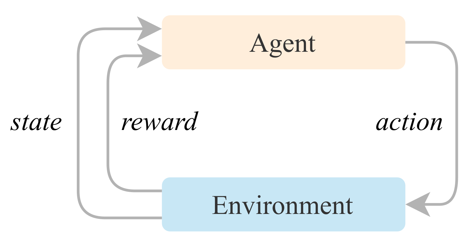
Figure 1.
General reinforcement learning model.
Figure 1.
General reinforcement learning model.
Figure 2.
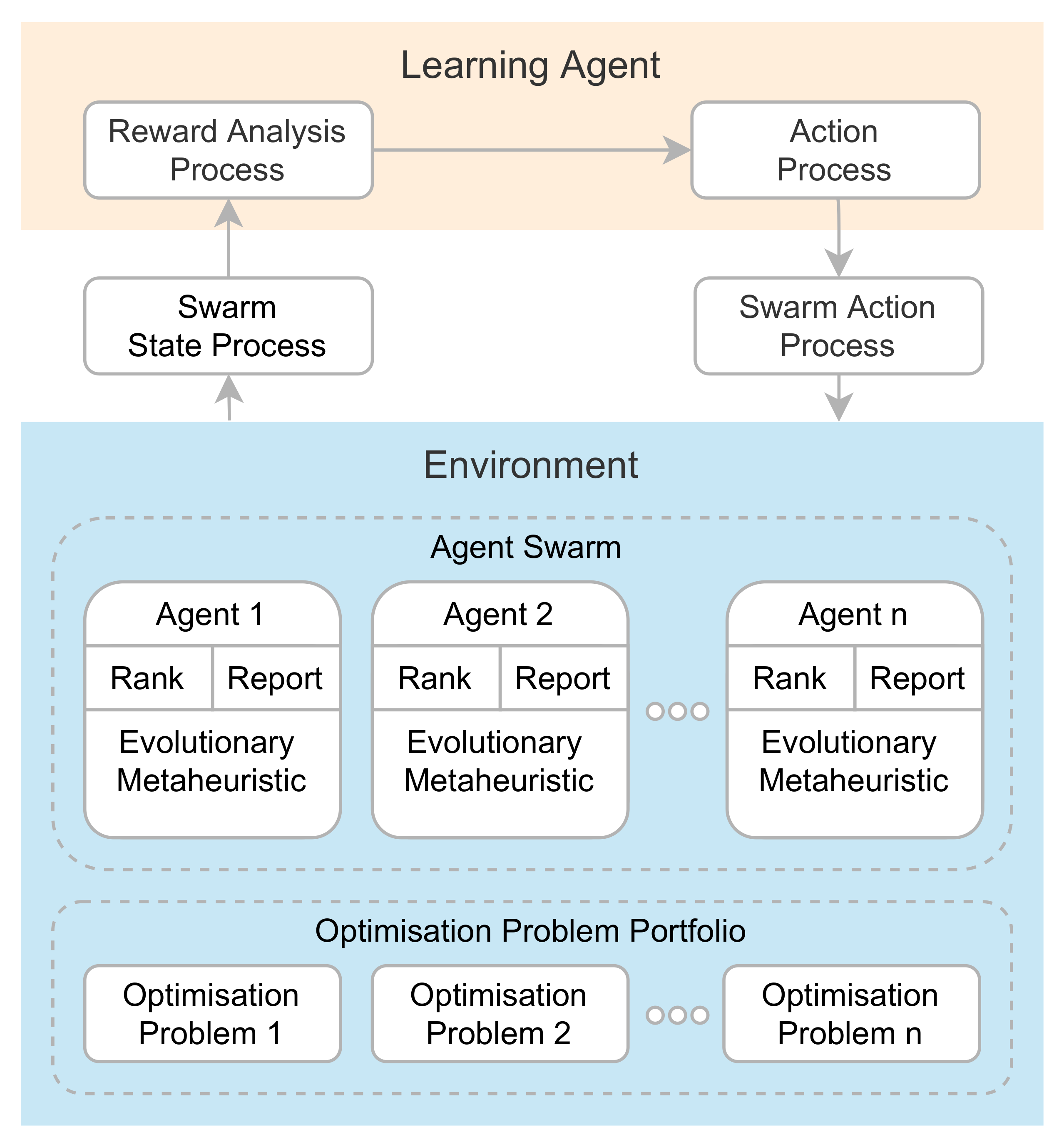
Proposed AutoMH framework for the automatic creation of metaheuristics.
Figure 2.
Proposed AutoMH framework for the automatic creation of metaheuristics.
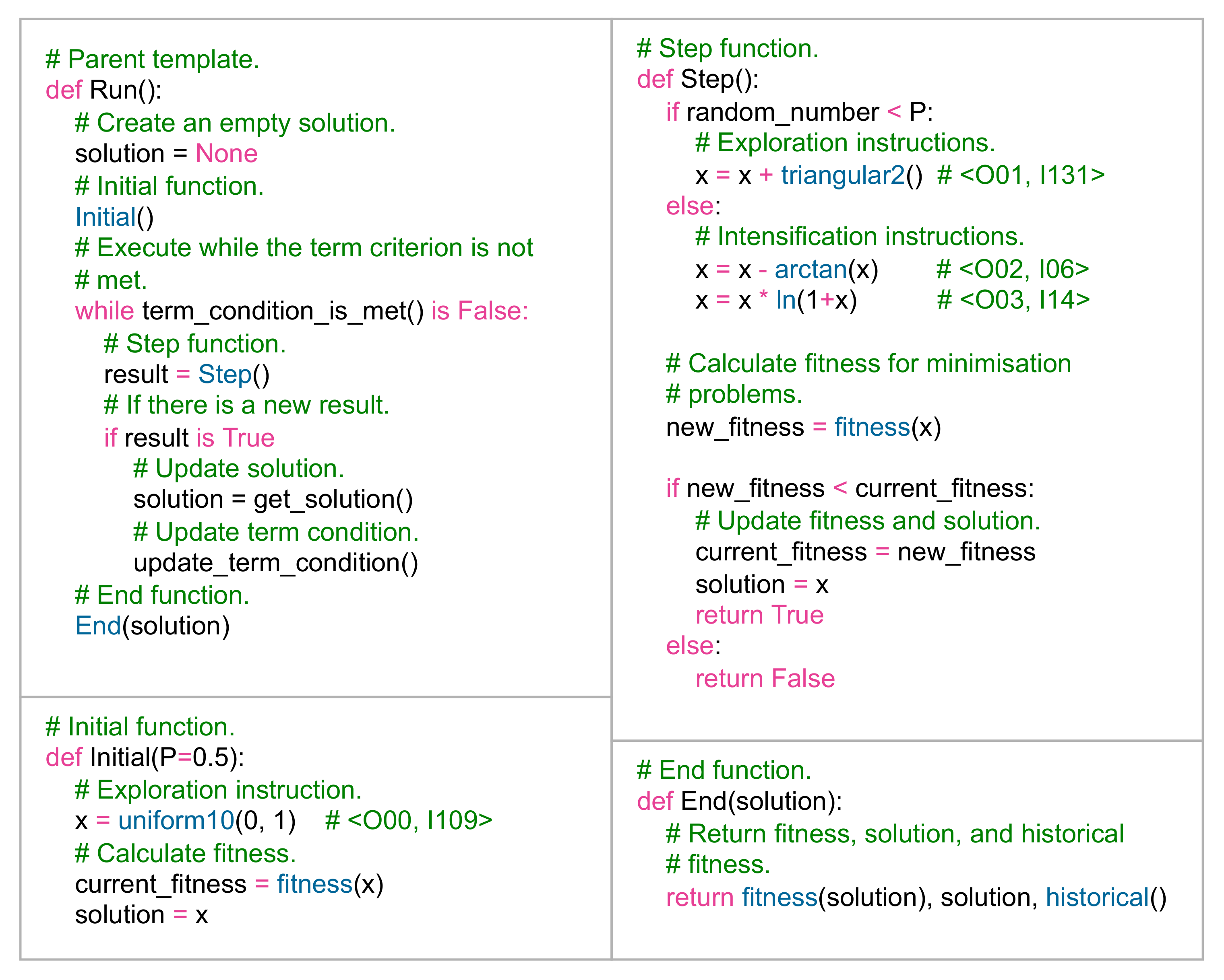
Figure 3.
Metaheuristic template .
Figure 3.
Metaheuristic template .
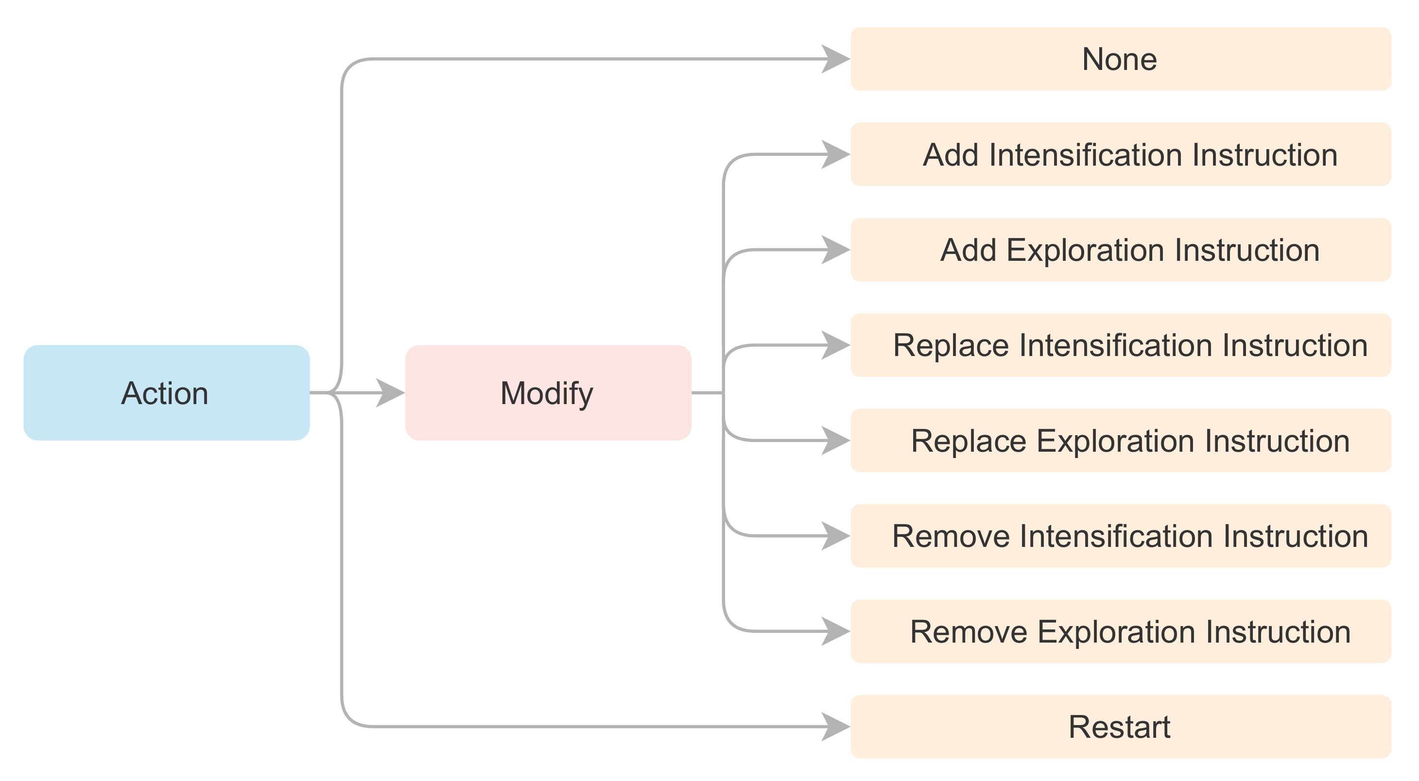
Figure 4.
Summary of the allowed action-space for the Learning Agent.
Figure 4.
Summary of the allowed action-space for the Learning Agent.
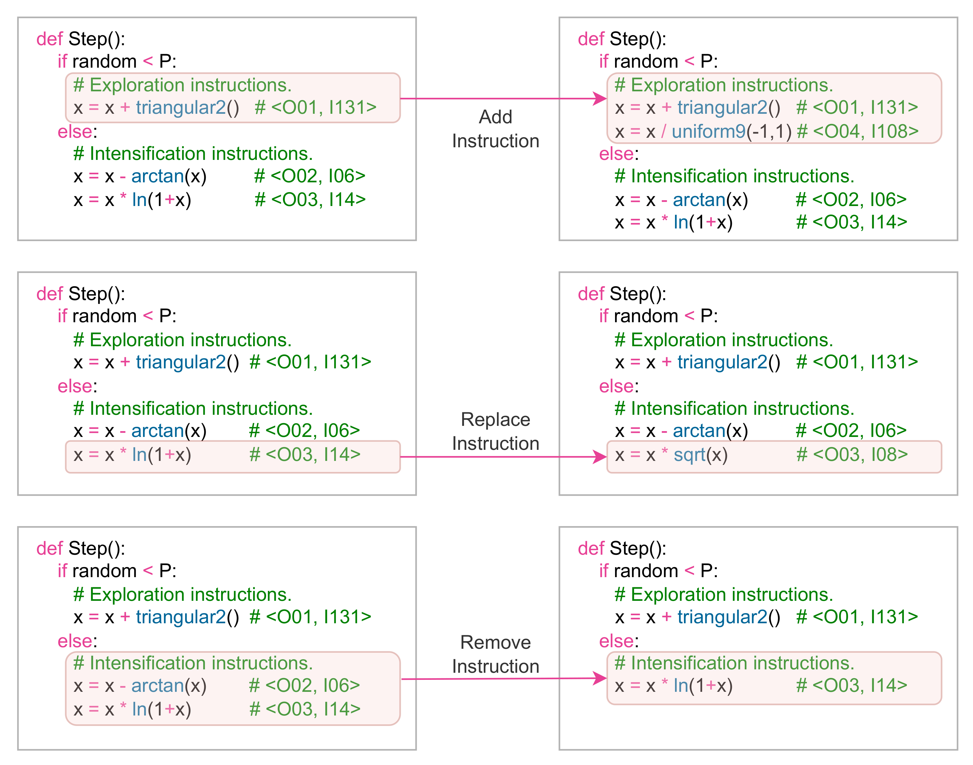
Figure 5.
Example of modifications in the structure of the metaheuristic algorithm.
Figure 5.
Example of modifications in the structure of the metaheuristic algorithm.
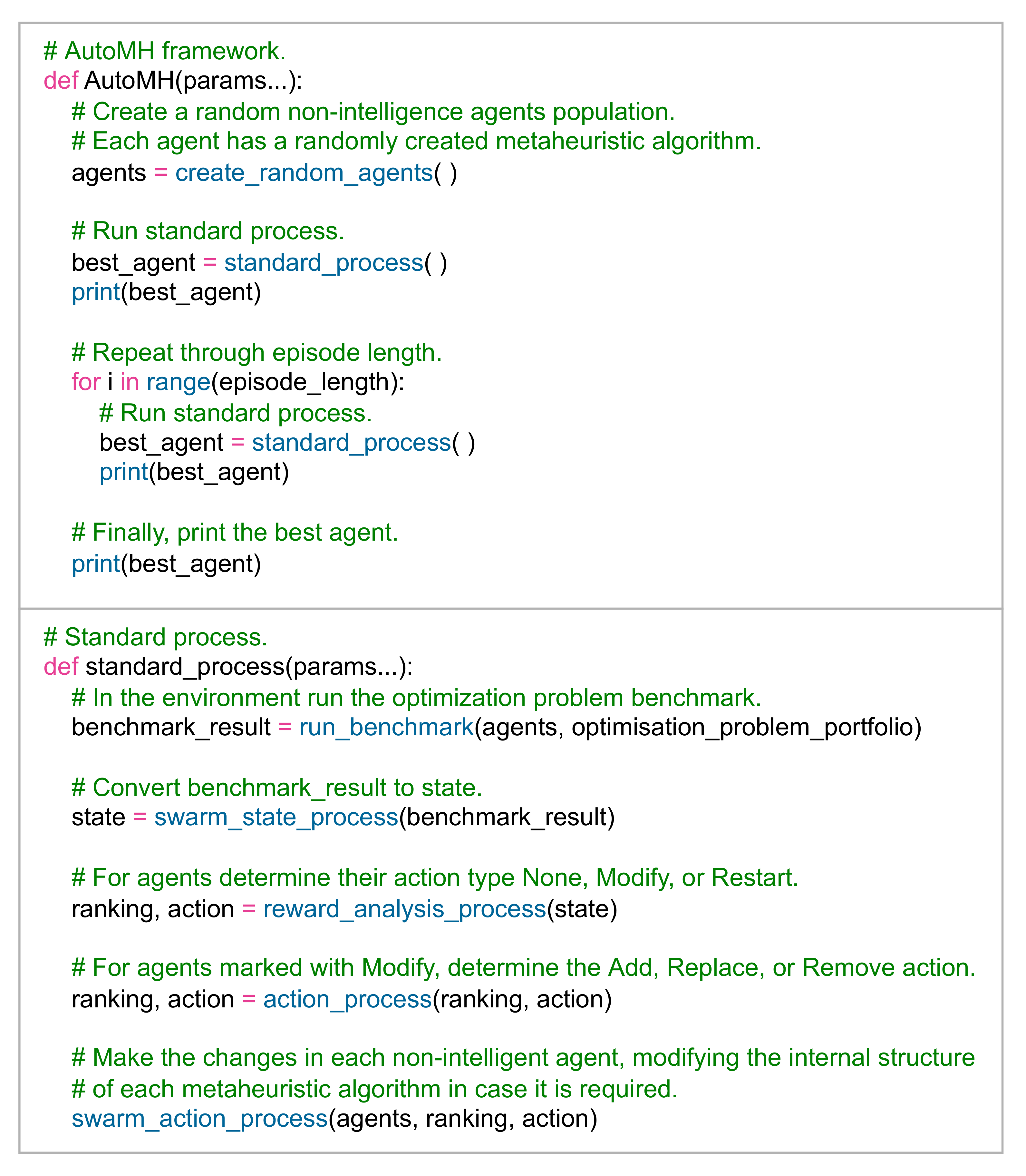
Figure 6.
AutoMH framework pseudocode.
Figure 6.
AutoMH framework pseudocode.
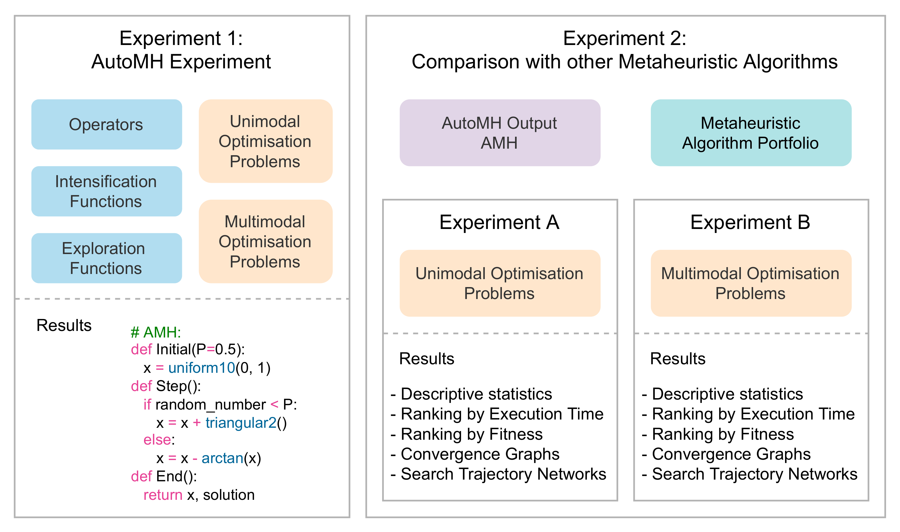
Figure 7.
Overview of experiments.
Figure 7.
Overview of experiments.
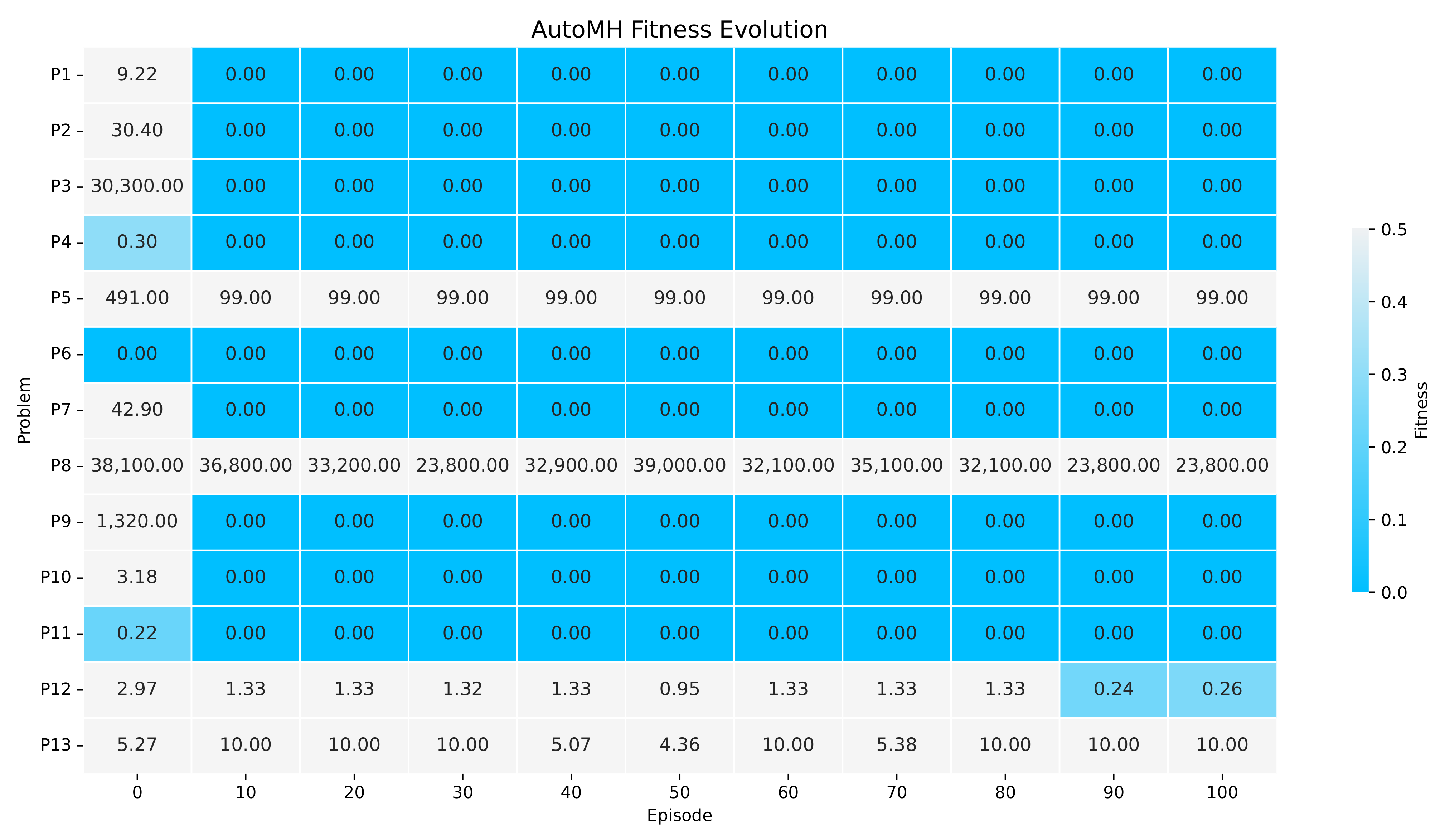
Figure 8.
The Figure showing the evolution of fitness during the 100 episodes of execution of AutoMH framework. The figure summarises the episodes 10 by 10.
Figure 8.
The Figure showing the evolution of fitness during the 100 episodes of execution of AutoMH framework. The figure summarises the episodes 10 by 10.
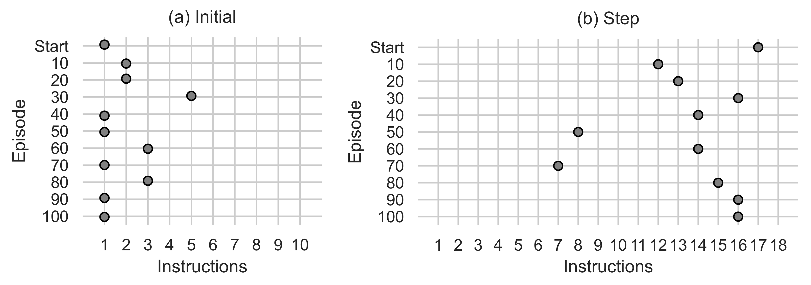
Figure 9.
(a) Shows the number of instructions used in the Initial function. (b) Shows the number of instructions used in the Step function.
Figure 9.
(a) Shows the number of instructions used in the Initial function. (b) Shows the number of instructions used in the Step function.
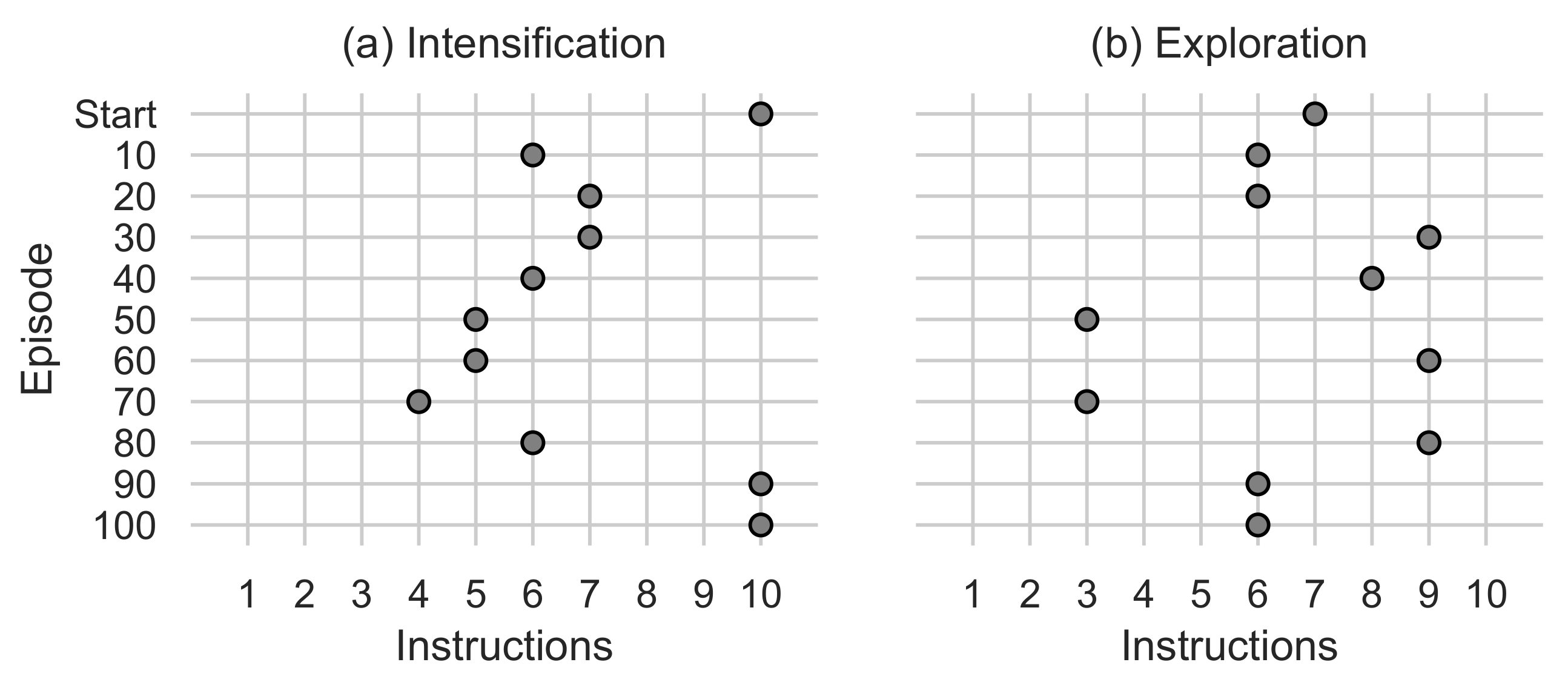
Figure 10.
(a) Shows the number of intensification instructions used by the Step function. (b) Shows the number of exploration instructions used by the Step function.
Figure 10.
(a) Shows the number of intensification instructions used by the Step function. (b) Shows the number of exploration instructions used by the Step function.
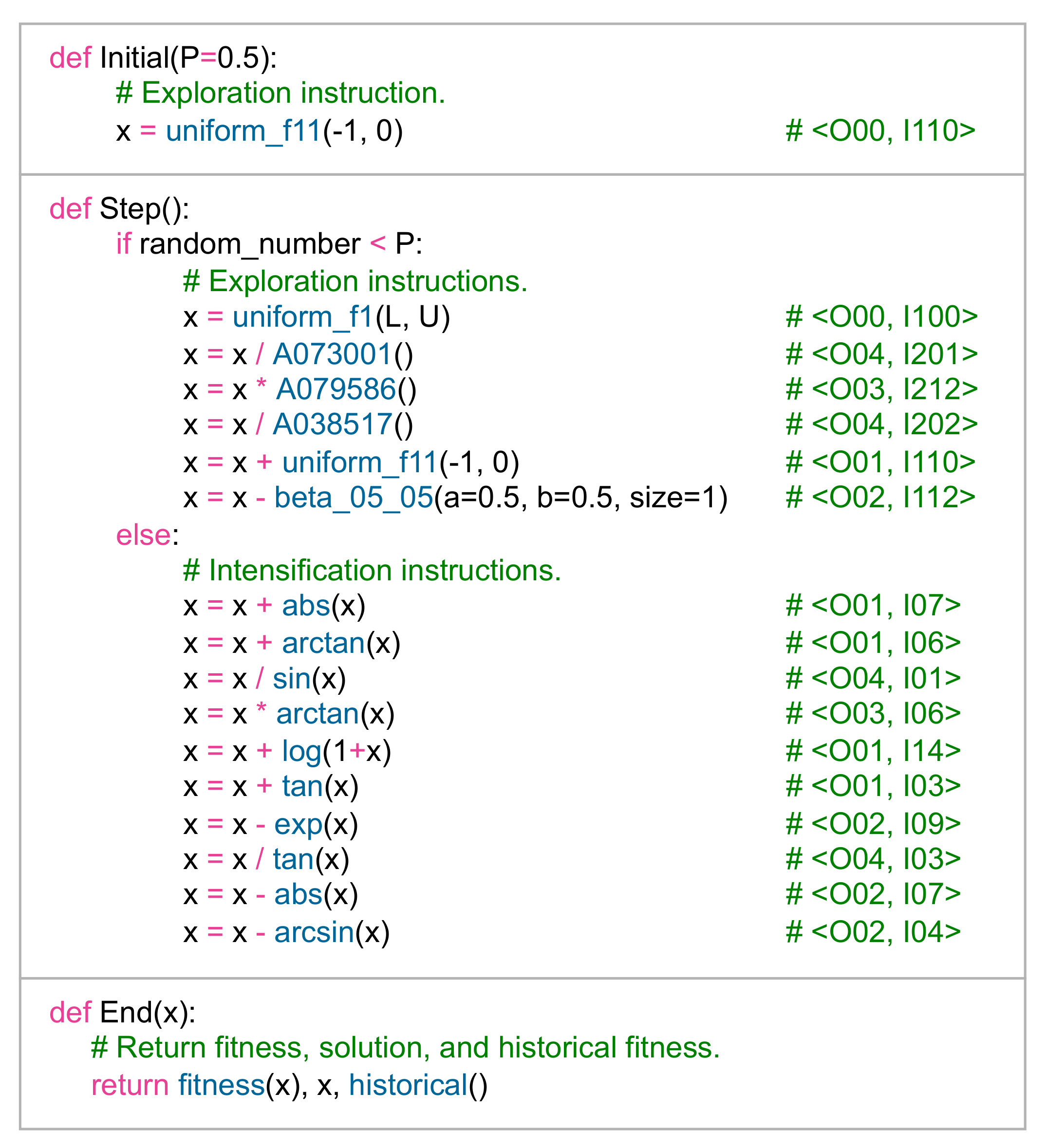
Figure 11.
Best algorithm found when running the AutoMH framework.
Figure 11.
Best algorithm found when running the AutoMH framework.
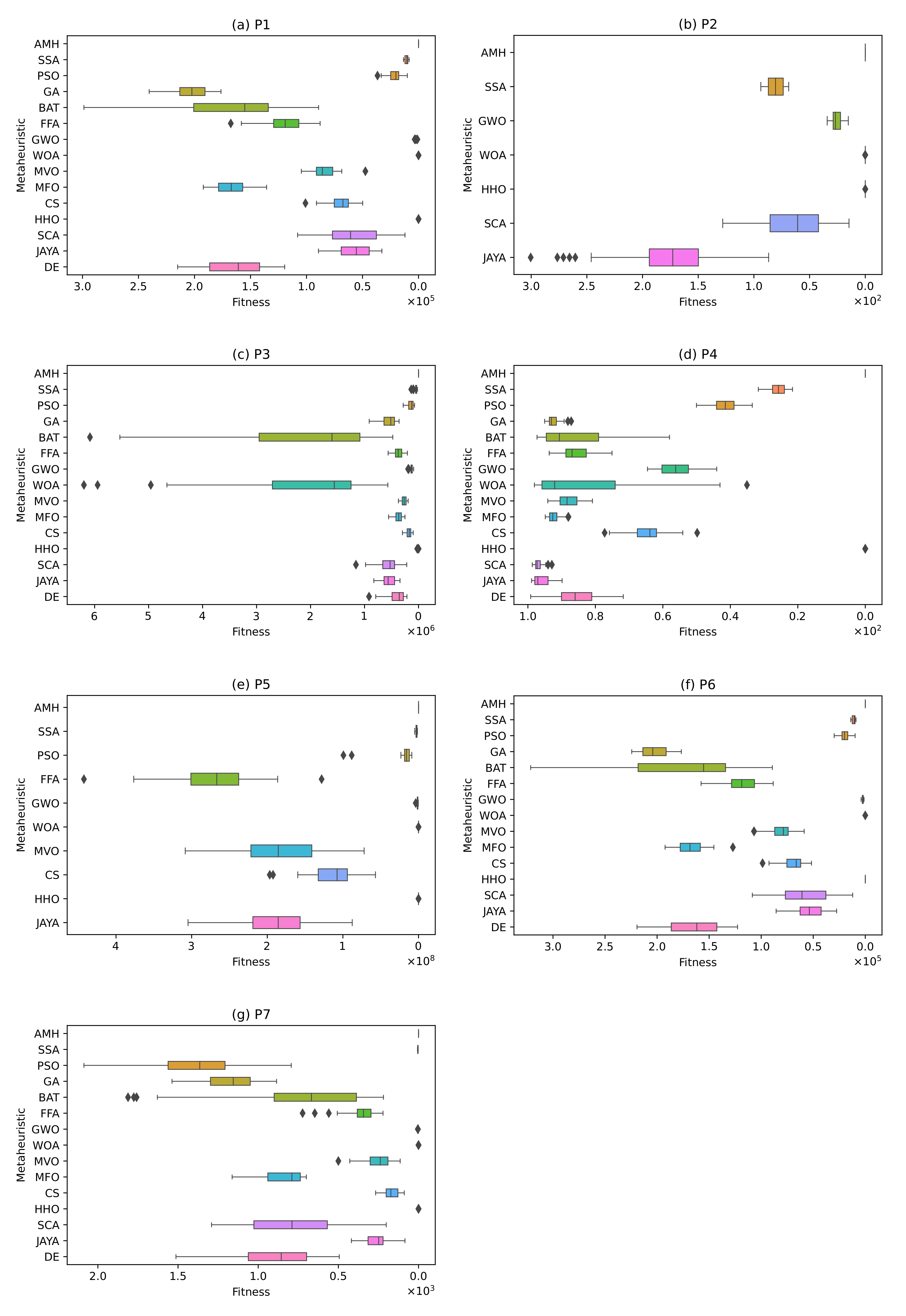
Figure 12.
The box plots for problems P1, P2, P3, P4, P5, P6, and P7.
Figure 12.
The box plots for problems P1, P2, P3, P4, P5, P6, and P7.
Figure 13.
A summary of the execution times of Experiment A. The figure is composed of a matrix and a vector of values that represent a measurement in seconds. The matrix represents the results by a set of cells. The cells indicate the duration of the 31 executions in which each metaheuristic algorithm executed each optimisation problem. The vector represents the total sums for each column of values in the matrix. The calculation is performed by adding together the times of the problems P1, P2, P3, P4, P5, P6, and P7.
Figure 14.
Summary of a ranking matrix between the algorithms in solving optimisation problems, considering mean fitness and execution time indicators. Each row represents the ranking among the 15 algorithms, ordered according to their performance at solving a problem P1, P2, P3, P4, P5, P6, or P7.
Figure 14.
Summary of a ranking matrix between the algorithms in solving optimisation problems, considering mean fitness and execution time indicators. Each row represents the ranking among the 15 algorithms, ordered according to their performance at solving a problem P1, P2, P3, P4, P5, P6, or P7.
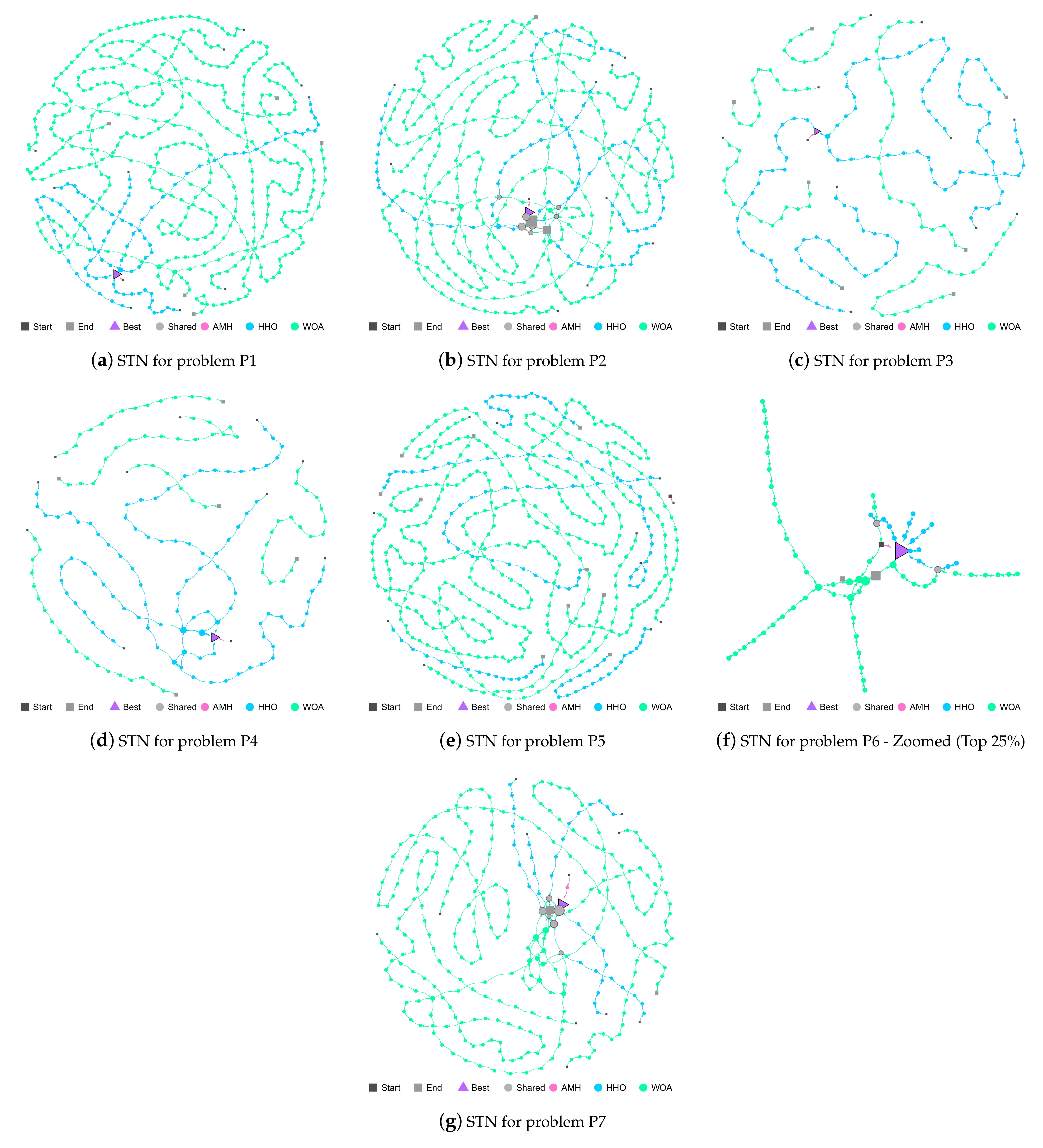
Figure 15.
Figures (a–g) show the Search Trajectory Networks of the AMH, HHO, and WOA algorithms for problems P1, P2, P3, P4, P5, P6, and P7, respectively. The squares indicate the start and end locations of the algorithm executions. The triangle node is the best-found solution.The circles represent the nodes of algorithms AMH, HHO, and WOA. Each algorithm has a default colour for each circular node. If a circular node is shared by more than one algorithm, it is depicted in light grey.
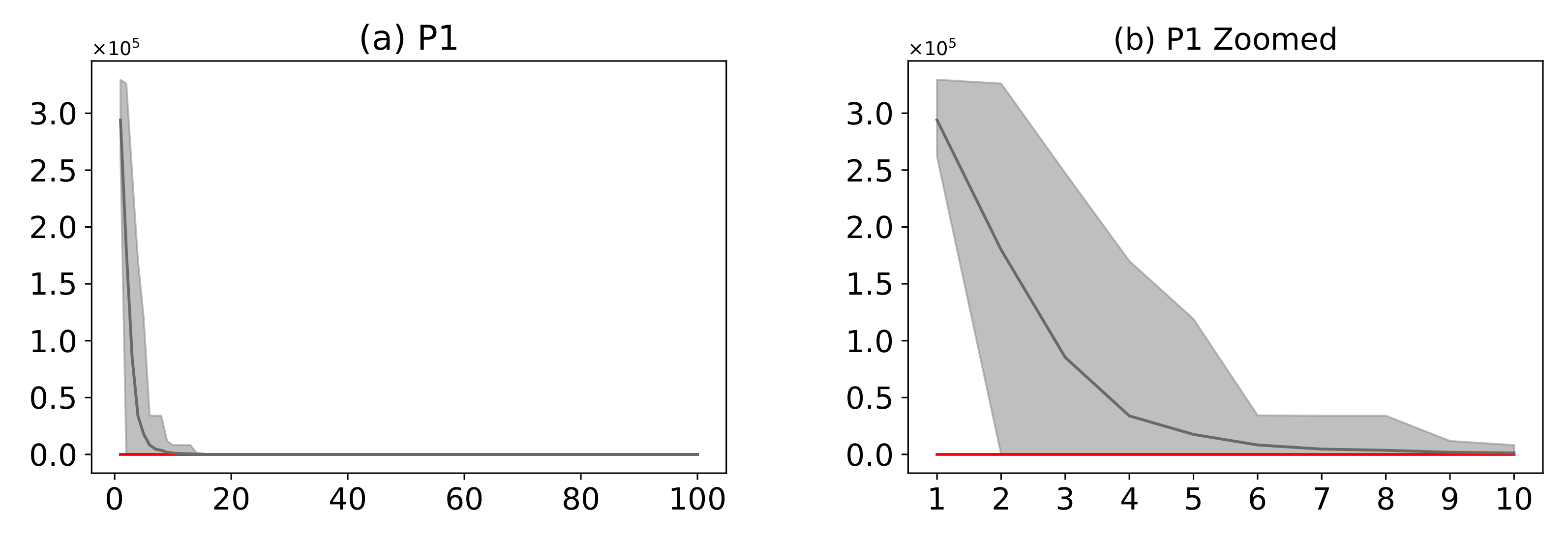
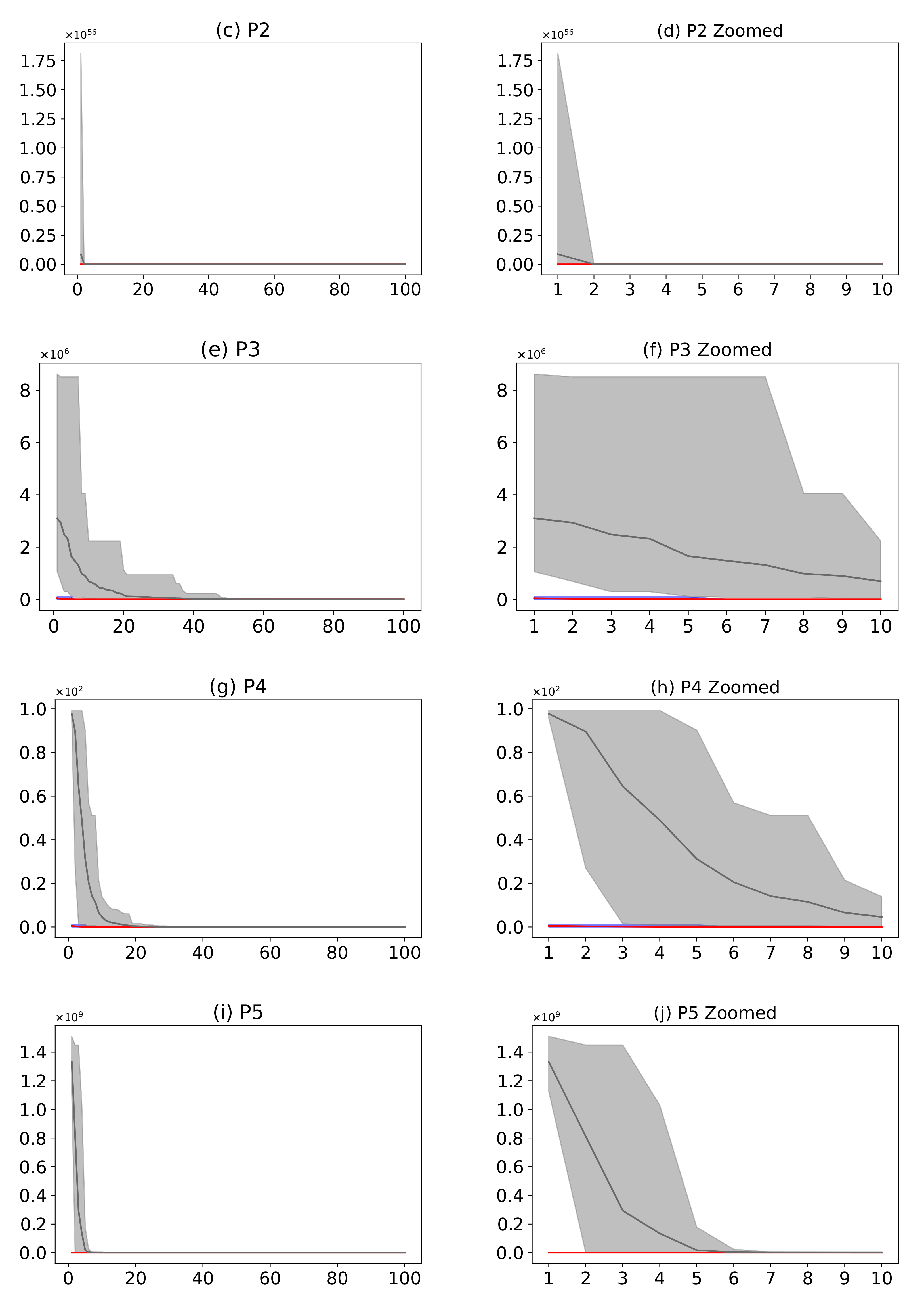
Figure 16.
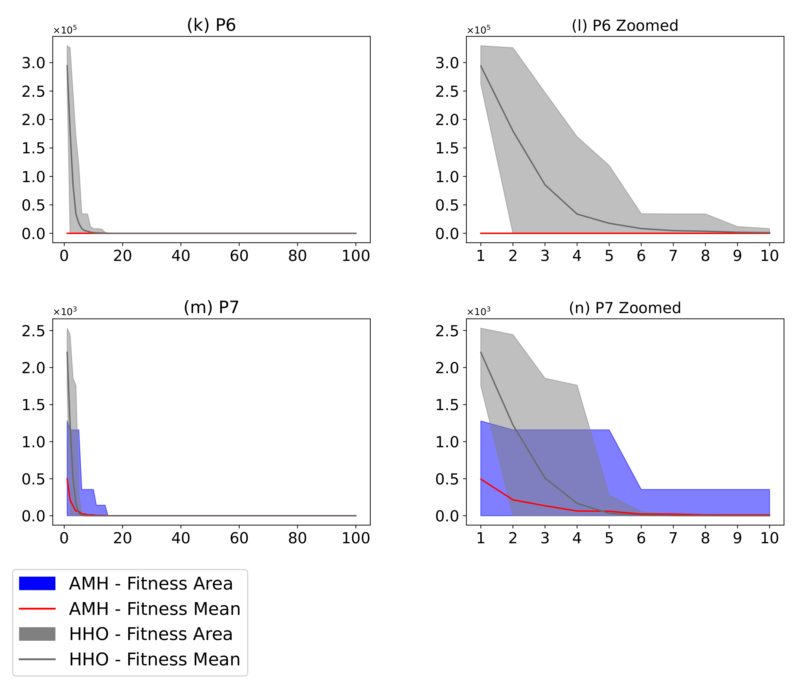
(Plots a,c,e,g,i,k,m) describe the convergence curves of the AMH and HHO algorithms for problems P1, P2, P3, P4, P5, P6, and P7; (Plots b,d,f,h,j,l,n) describe an enlarged view of the convergence curve from iteration 1 to 10. The x-axis indicates the number of iterations, and the y-axis indicates fitness. The areas represent the minimum and maximum fitness values obtained in each iteration for each algorithm. The lines represent the mean fitness value of each iteration. The information of the 31 executions is included.
Figure 16.
(Plots a,c,e,g,i,k,m) describe the convergence curves of the AMH and HHO algorithms for problems P1, P2, P3, P4, P5, P6, and P7; (Plots b,d,f,h,j,l,n) describe an enlarged view of the convergence curve from iteration 1 to 10. The x-axis indicates the number of iterations, and the y-axis indicates fitness. The areas represent the minimum and maximum fitness values obtained in each iteration for each algorithm. The lines represent the mean fitness value of each iteration. The information of the 31 executions is included.
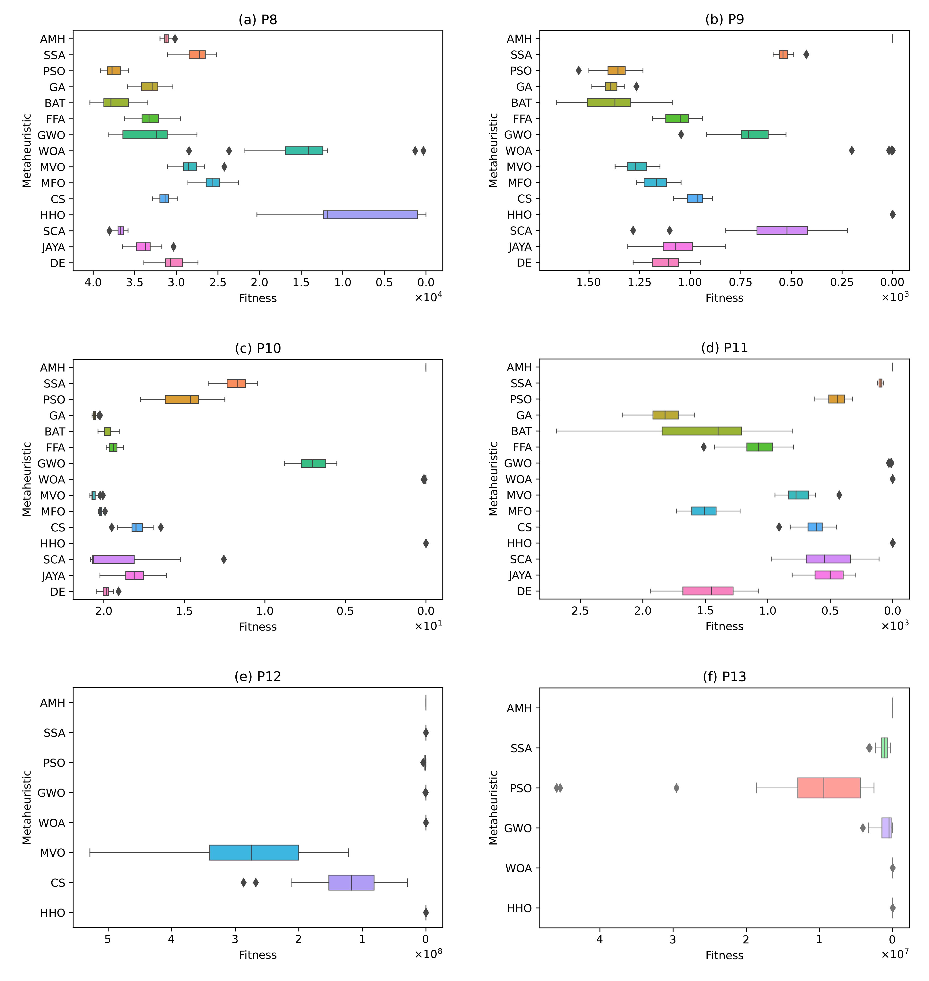
Figure 17.
The box plots for problems P8, P9, P10, P11, P12, and P13.
Figure 17.
The box plots for problems P8, P9, P10, P11, P12, and P13.
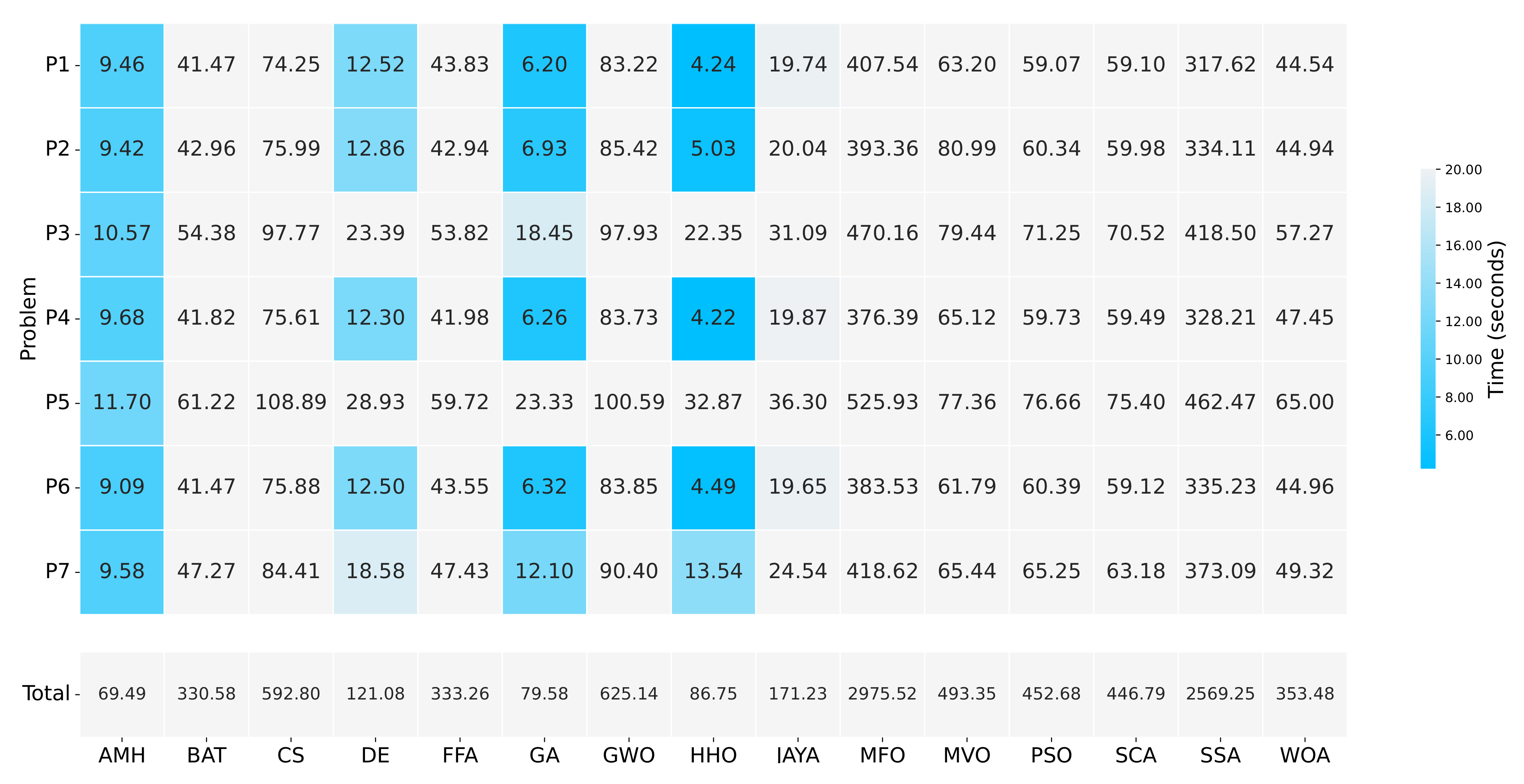
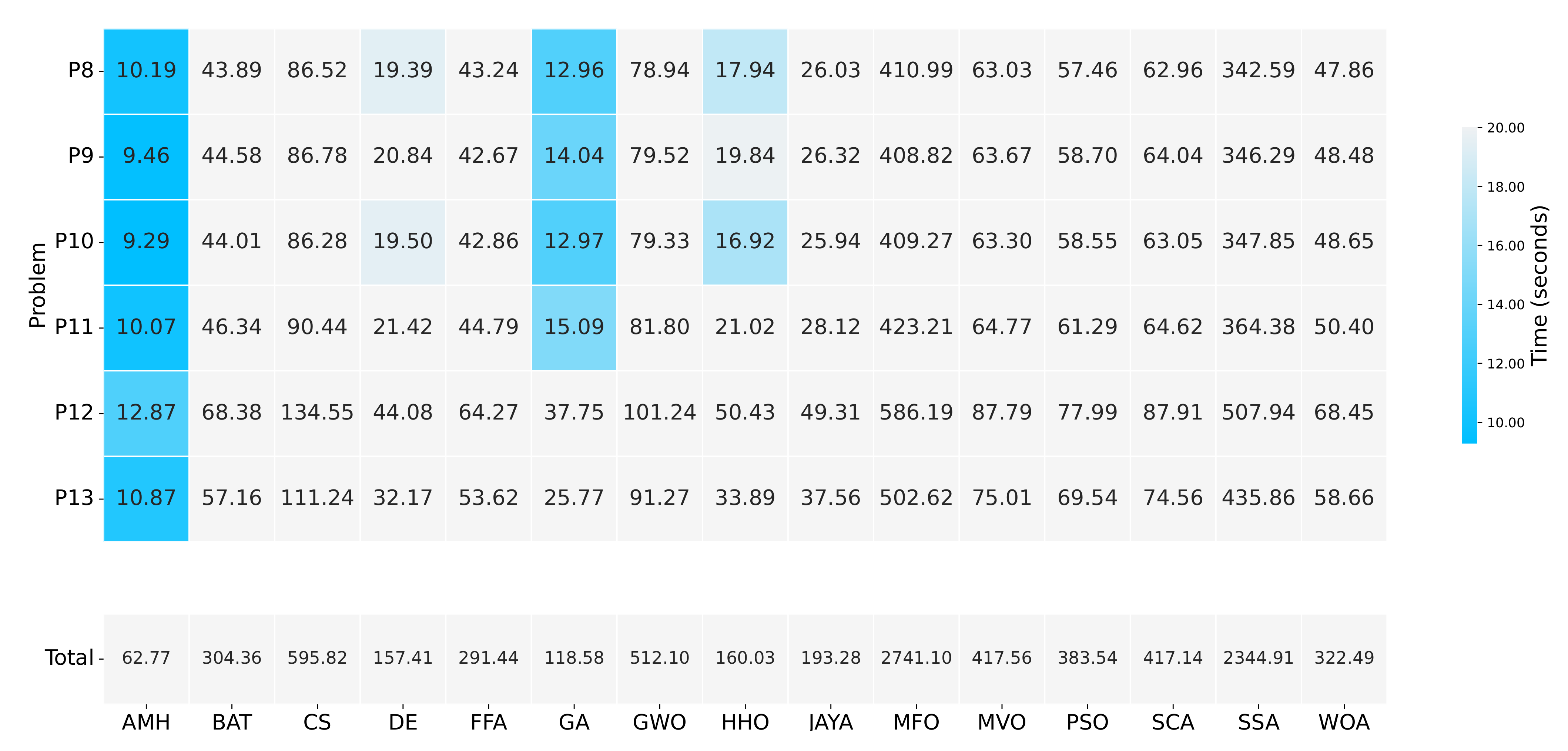
Figure 18.
A summary of the execution times of Experiment B. The figure is composed of a matrix and a vector of values that represent a measurement in seconds. The matrix represents the results by a set of cells. The cells indicate the duration of the 31 executions in which each metaheuristic algorithm executed each optimisation problem. The vector represents the total sum for each column of values in the matrix. The calculation is performed by adding together the time values of the problems P8, P9, P10, P11, P12, and P13.
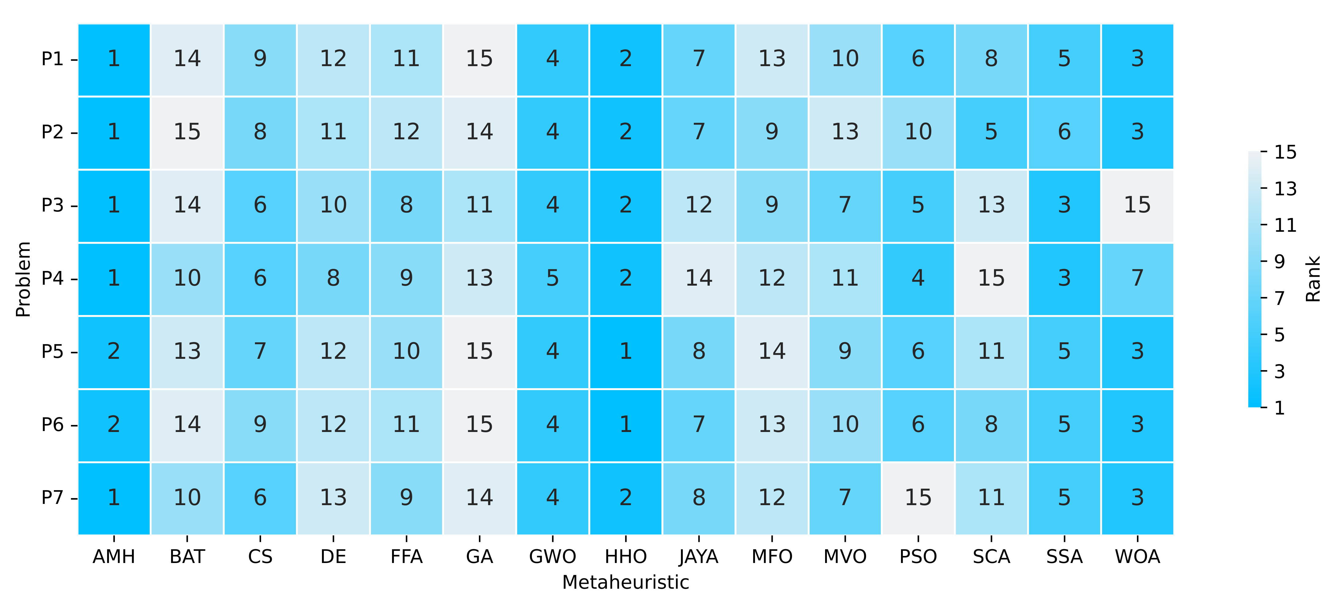
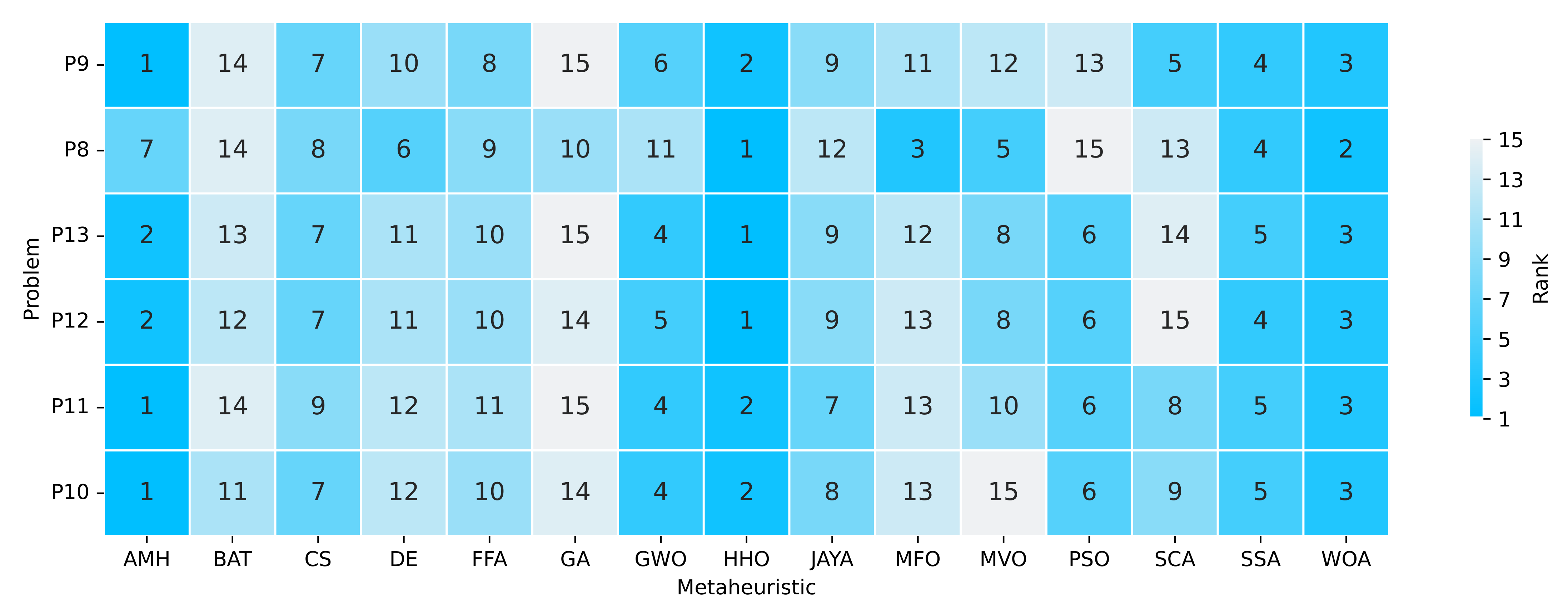
Figure 19.
Summary of a ranking matrix between the algorithms in solving optimisation problems, considering mean fitness and execution time indicators. Each row represents the ranking among the 15 algorithms ordered by efficiency in solving a problem P8, P9, P10, P11, P12, and P13.
Figure 19.
Summary of a ranking matrix between the algorithms in solving optimisation problems, considering mean fitness and execution time indicators. Each row represents the ranking among the 15 algorithms ordered by efficiency in solving a problem P8, P9, P10, P11, P12, and P13.
Figure 20.
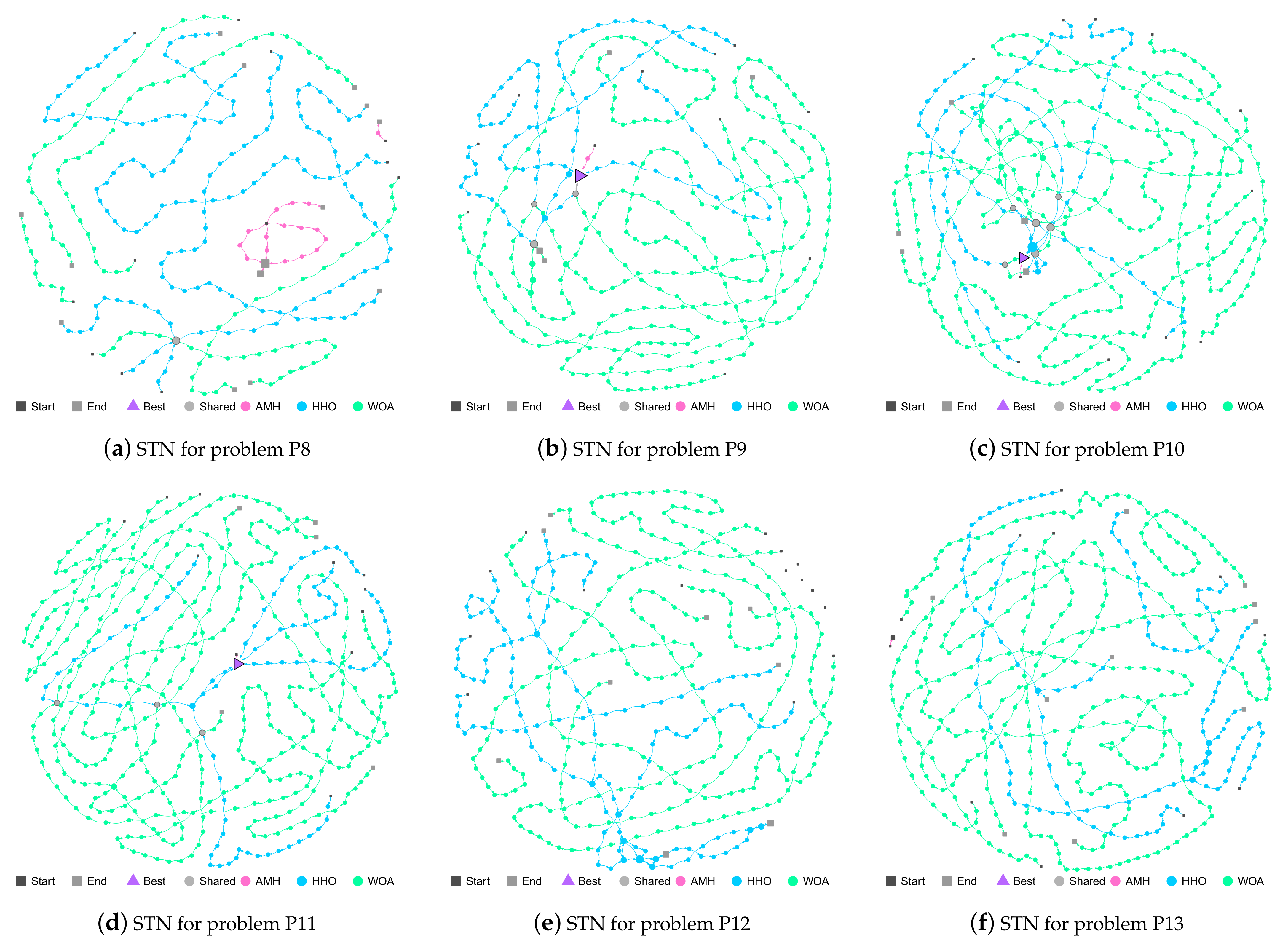
(a–f) Search Trajectory Networks of the AMH, HHO, and WOA algorithms for problems P8, P9, P10, P11, P12, and P13, respectively. The squares indicate the start and end locations of the algorithm executions. The triangle node is the best-found solution. The circles represent the nodes of algorithms AMH, HHO, and WOA. Each algorithm has a default colour for each circular node. If a circular node is shared by more than one algorithm, it is depicted in light grey.
Figure 20.
(a–f) Search Trajectory Networks of the AMH, HHO, and WOA algorithms for problems P8, P9, P10, P11, P12, and P13, respectively. The squares indicate the start and end locations of the algorithm executions. The triangle node is the best-found solution. The circles represent the nodes of algorithms AMH, HHO, and WOA. Each algorithm has a default colour for each circular node. If a circular node is shared by more than one algorithm, it is depicted in light grey.
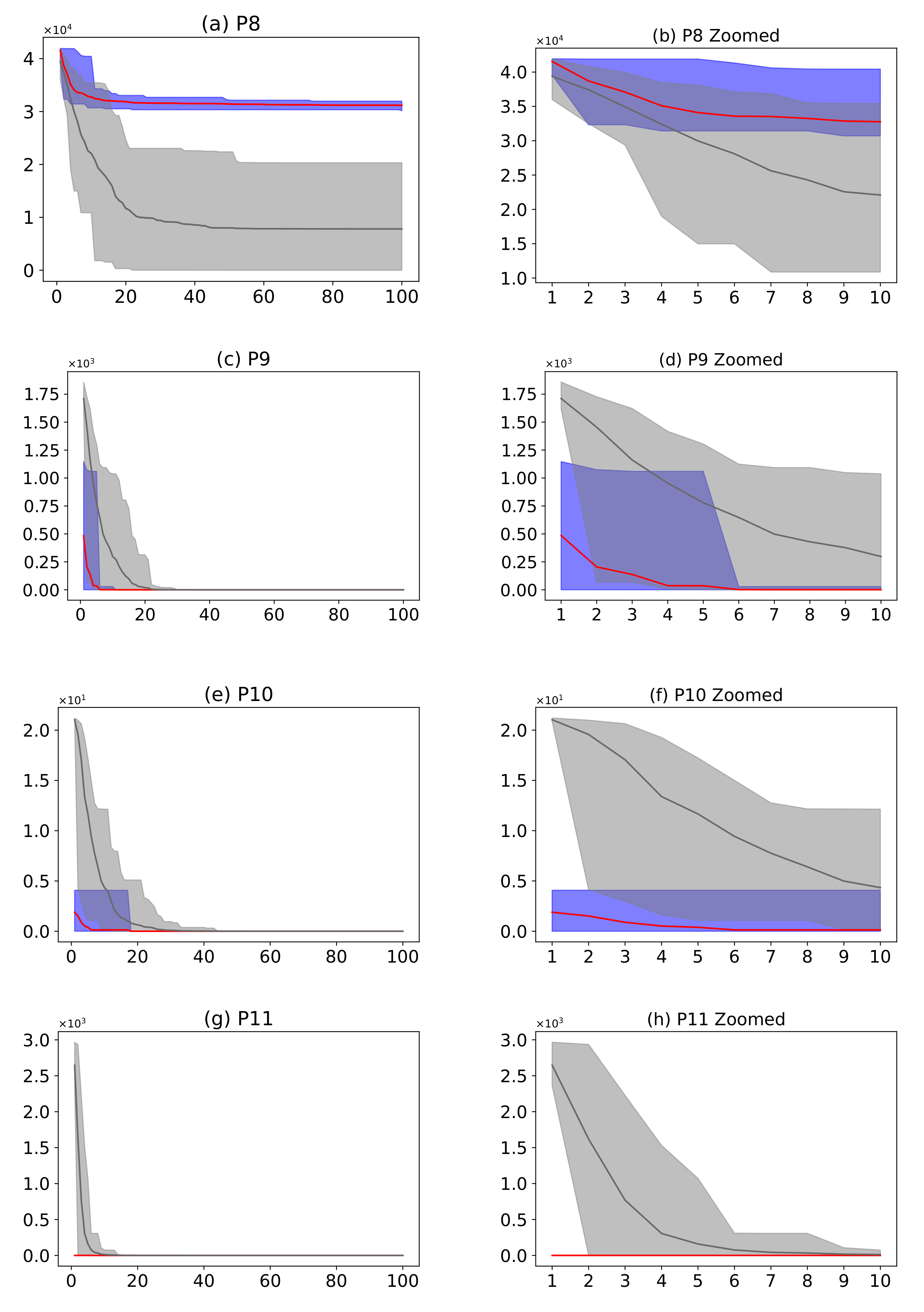
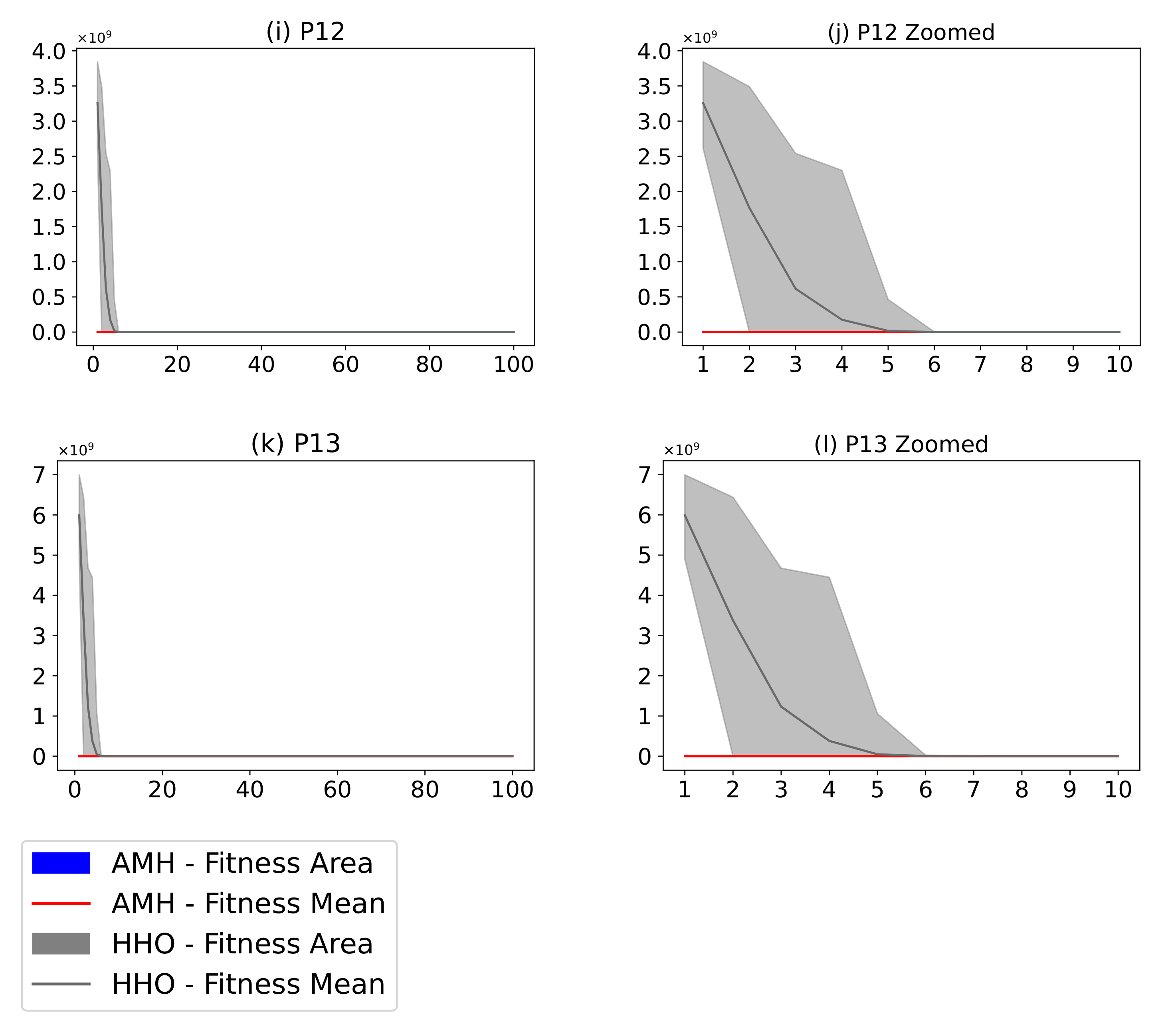
Figure 21.
(Plots a,c,e,g,i,k) describe the convergence curves of the AMH and HHO algorithms for problems P1, P2, P3, P4, P5, P6, and P7; (Plots b,d,f,h,j,l) describe an enlarged view of the convergence curve from iteration 1 to 10. The x-axis indicates the number of iterations, and the y-axis indicates fitness. The areas represent the minimum and maximum fitness values obtained in each iteration for each algorithm. The lines represent the mean fitness value of each iteration. Information regarding the 31 executions is included.
Table 1.
List of unimodal continuous optimisation problems.
Table 1.
List of unimodal continuous optimisation problems.
| Identifier | Function Name | Domain | | | Details | Reference |
|---|
| P01 | Sphere | [−100, 100] | 0 | f(0, 0, …, 0) | Definition A1 | [19,20] |
| P02 | Schwefel Function 2.22 | [−10, 10] | 0 | f(0, 0, …, 0) | Definition A2 | [20] |
| P03 | Schwefel Function 1.2 | [−100, 100] | 0 | f(0, 0, …, 0) | Definition A3 | [20] |
| P04 | Schwefel Function 2.21 | [−100, 100] | 0 | f(0, 0, …, 0) | Definition A4 | [20,21,22] |
| P05 | Rosenbrock’s | [−30, 30] | 0 | f(1, 1, …, 1) | Definition A5 | [19] |
| P06 | Step | [−100, 100] | 0 | f(),
| Definition A6 | [19,20] |
| P07 | Quartic | [−1.28, 1.28] | 0 | f(0, 0, …, 0) | Definition A7 | [20] |
Table 2.
List of multimodal continuous optimisation problems.
Table 2.
List of multimodal continuous optimisation problems.
| Identifier | Function Name | Domain | | | Details | Reference |
|---|
| P08 | Schwefel Function 2.26 | [−500, 500] | 0 | f(4.21 × 10 2, …, 4.21 × 10 2) | Definition A8 | [20] |
| P09 | Rastrigin | [−5.12, 5.12] | 0 | f(0, 0, … 10 2, 0) | Definition A9 | [23] |
| P10 | Ackley | [−32, 32] | 0 | f(0, 0, …, 0) | Definition A10 | [19] |
| P11 | Griewank | [−600, 600] | 0 | f(0, 0, …, 0) | Definition A11 | [24] |
| P12 | Generalized Penalized Function 1 | [−50, 50] | 0 | f(−1, −1, …, −1) | Definition A12 | [23] |
| P13 | Generalized Penalized Function 2 | [−50, 50] | 0 | f(1, 1, …, 1) | Definition A13 | [23] |
Table 3.
List of operators.
Table 3.
List of operators.
| Identifier | Name | Math | Code |
|---|
| O00 | None | x ← x | x = x |
| O01 | Plus | x ← x + f(x)
| x = x + f(x) |
| O02 | Subtract | x ← x − f(x)
| x = x − f(x) |
| O03 | Multiply | x ← x * f(x)
| x = x * f(x) |
| O04 | Divide | x ← | x = x/f(x) |
Table 4.
List of basic functions.
Table 4.
List of basic functions.
| Identifier | Name | Function | Code |
|---|
| I01 | Sine | f(x) = sin(x)
| x = sin(x) |
| I02 | Cosine | f(x) = cos(x)
| x = cos(x) |
| I03 | Tangent | f(x) = tan(x)
| x = tan(x) |
| I04 | Inverse Sine | f(x) = arcsin(x)
| x = arcsin(x) |
| I05 | Inverse Cosine | f(x) = arccos(x)
| x = arccos(x) |
| I06 | Inverse Tangent | f(x) = arctan(x)
| x = arctan(x) |
| I07 | Absolute | f(x) = |x|
| x = abs(x) |
| I08 | Square root | f(x) = | x = sqrt(x) |
| I09 | Exponential function | f(x) = ex | x = exp(x) |
| I10 | Exponential function minus 1 | f(x) = ex − 1
| x = exp1(x) |
| I11 | Natural logarithm | f(x) = ln(x)
| x = ln(x) |
| I12 | Base-2 logarithm of x | f(x) = log2(x)
| x = log2(x) |
| I13 | Base-10 logarithm of x | f(x) = log10(x)
| x = log10(x) |
| I14 | Natural logarithm of one plus | f(x) = ln(1 + x)
| x = ln(1 + x) |
Table 5.
List of random number functions.
Table 5.
List of random number functions.
| Identifier | Name | Function | Code | Description |
|---|
| I100 | Uniform F1 | Uf1 ~ (l, u)
| x = uniform1(l, u) | |
| I101 | Uniform F2 | Uf2 ~ (l, u)
| x = uniform2(l, u) | u = lb + (ub − lb)/2 |
| I102 | Uniform F3 | Uf3 ~ (l, u)
| x = uniform3(l, u) | l = lb + (ub − lb)/2 |
| I103 | Uniform F4 | Uf4 ~ (l, u)
| x = uniform4(l, u) | l = lb + (ub − lb)/3
u = lb + (ub − lb)/3*2 |
| I104 | Uniform F5 | Uf5 ~ (l, u)
| x = uniform5(l, u) | u = lb + (ub − lb)/4 |
| I105 | Uniform F6 | Uf6 ~ (l, u)
| x = uniform6(l, u) | l = lb + (ub − lb)/4
u = lb + (ub − lb)/2 |
| I106 | Uniform F7 | Uf7 ~ (l, u)
| x = uniform7(l, u) | l = lb + (ub − lb)/2
u = lb + (ub − lb)/4*3 |
| I107 | Uniform F8 | Uf8 ~ (l, u)
| x = uniform8(l, u) | l = lb + (ub − lb)/4*3 |
| I108 | Uniform F9 | Uf9 ~ (−1, 1)
| x = uniform9(−1, 1) | |
| I109 | Uniform F10 | Uf10 ~ (0, 1)
| x = uniform10(0, 1) | |
| I110 | Uniform F11 | Uf11 ~ (−1, 1)
| x = uniform11(−1, 0) | |
| I111 | Uniform F12 | Uf12 ~ (0.5, 0.5)
| x = uniform12(0.5, 0.5) | |
| I112 | Beta F1 | Bf1 ~ (0.5, 0.5, 1)
| x = beta1(0.5, 0.5, 1) | |
| I113 | Beta F2 | Bf2 ~ (5, 1, 1)
| x = beta2(5, 1, 1) | |
| I114 | Beta F3 | Bf3 ~ (1, 3, 1)
| x = beta3(1, 3, 1) | |
| I115 | Beta F4 | Bf4 ~ (2, 2, 1)
| x = beta4(2, 2, 1) | |
| I116 | Beta F5 | Bf5 ~ (2, 5, 1)
| x = beta5(2, 5, 1) | |
| I117 | Triangular F1 | Tf1 ~ (lb, m, ub)
| x = triangular1(lb, m, ub) | m = lb + (ub − lb)/2 |
| I118 | Triangular F2 | Tf2 ~ (lb, m, ub)
| x = triangular2(lb, m, ub) | m = lb + (ub − lb)/4 |
| I119 | Triangular F3 | Tf3 ~ (lb, m, ub)
| x = triangular3(lb, m, ub) | m = lb + (ub − lb)/3 |
| I120 | Triangular F4 | Tf4 ~ (lb, m, ub)
| x = triangular4(lb, m, ub) | m = lb + ((ub − lb)/4)*3 |
| I121 | Triangular F5 | Tf5 ~ (lb, m, ub)
| x = triangular5(lb, m, ub) | m = lb + ((ub − lb)/3)*2 |
Table 6.
List of constants.
Table 6.
List of constants.
| ID | Name | Symbol | Value | Code |
|---|
| I200 | Meissel–Mertens | | 0.26149 72128 47642 78375 54268 38608 69585 | A077761( ) |
| I201 | Bernstein’s | | 0.28016 94990 23869 13303 | A073001( ) |
| I202 | Gauss–Kuzmin–Wirsing | | 0.30366 30028 98732 65859 74481 21901 55623 | A038517( ) |
| I203 | Hafner–Sarnak–McCurley | | 0.35323 63718 54995 98454 35165 50432 68201 | A085849( ) |
| I204 | Omega | | 0.56714 32904 09783 87299 99686 62210 35554 | A030178( ) |
| I205 | Euler–Mascheroni | | 0.57721 56649 01532 86060 65120 90082 40243 | A001620( ) |
| I206 | Twin prime | | 0.66016 18158 46869 57392 78121 10014 55577 | A005597( ) |
| I207 | Conway’s | | 1.30357 72690 34296 39125 70991 12152 55189 | A014715( ) |
| I208 | Ramanujan–Soldner | | 1.45136 92348 83381 05028 39684 85892 02744 | A070769( ) |
| I209 | Golden ratio | | 1.61803 39887 49894 84820 45868 34365 63811 | A001622( ) |
| I210 | Euler’s number | e | 2.71828 18284 59045 23536 02874 71352 66249 | A001113( ) |
| I211 | Pi | | 3.14159 26535 89793 23846 26433 83279 50288 | A000796( ) |
| I212 | Reciprocal Fibonacci | | 3.35988 56662 43177 55317 20113 02918 92717 | A079586( ) |
Table 7.
Parameters used in the AutoMH experiment.
Table 7.
Parameters used in the AutoMH experiment.
| ID | Name | Description | Value |
|---|
| T01 | Evolutionary Agents | The number of non-intelligent agents in the swarm. | |
| T02 | Evolutionary Iterations (Episode) | The number of times the agents in the swarm have to repeat the optimisation tests once the structure of their algorithm is modified by the learning agent. | |
| T03 | Mutation Selection | The mutation is carried out by randomly choosing an action of the type Add, Replace, and Remove for the Modified case. | |
| T04 | MH Iteration | The maximum number of iterations that the metaheuristic executes. | |
| T05 | MH Execution | The number of times the metaheuristic is executed. | |
| T05 | MH Probability | The probability of choosing intensification or exploration in the Step function. | |
| T06 | Dimension | The dimension of optimisation problems. | |
| T07 | Operator Initial | The operators allowed to modify the metaheuristic template in the Initial function. | |
| T08 | Initial Functions | The Initial functions allowed for modifying the metaheuristic template in the Initial function. | |
| T09 | Operator Exploration | The operators allowed to modify the metaheuristic template in the step function. | |
| T10 | Exploration Functions | The exploration instructions allowed for modifying the metaheuristic template in the step function. | |
| T11 | Operator Intensification | The operators allowed to modify the metaheuristic template in the step function. | |
| T12 | Intensification Functions | The intensification functions allowed for the modification of the metaheuristic template in the step function. | |
| T13 | Initial quantity | Minimum and maximum number of operators allowed in the generated metaheuristic | . |
| T14 | Exploration quantity | Minimum and maximum amount of exploration instructions allowed in the generated metaheuristic | . |
| T15 | Intensification quantity | Minimum and maximum amount of intensification instructions allowed in the generated metaheuristic | . |
Table 8.
Experiment A: Statistical Summary.
Table 8.
Experiment A: Statistical Summary.
| Metaheuristic | Type | P1 | P2 | P3 | P4 | P5 | P6 | P7 |
|---|
| AMH | mean | 0.00 | 0.00 | 0.00 | 0.00 | 9.90 × 10 | 0.00 | 0.00 |
| std | 0.00 | 0.00 | 0.00 | 0.00 | 0.00 | 0.00 | 0.00 |
| BAT | mean | 1.74 × 10 | 1.54 × 10 | 2.16 × 10 | 8.67 × 10 | 5.51 × 10 | 1.80 × 10 | 7.56 × 10 |
| std | 6.19 × 10 | 7.53 × 10 | 1.43 × 10 | 1.02 × 10 | 3.27 × 10 | 7.11 × 10 | 4.60 × 10 |
| CS | mean | 6.98 × 10 | 1.65 × 10 | 1.79 × 10 | 6.46 × 10 | 1.13 × 10 | 6.98 × 10 | 1.73 × 10 |
| std | 1.18 × 10 | 8.53 × 10 | 5.26 × 10 | 6.19 | 3.21 × 10 | 1.20 × 10 | 5.06 × 10 |
| DE | mean | 1.64 × 10 | 4.39 × 10 | 4.11 × 10 | 8.57 × 10 | 5.48 × 10 | 1.65 × 10 | 9.00 × 10 |
| std | 2.56 × 10 | 2.21 × 10 | 1.72 × 10 | 6.55 | 1.73 × 10 | 2.64 × 10 | 2.49 × 10 |
| FFA | mean | 1.19 × 10 | 4.06 × 10 | 3.80 × 10 | 8.59 × 10 | 2.72 × 10 | 1.18 × 10 | 3.63 × 10 |
| std | 1.71 × 10 | 2.20 × 10 | 9.36 × 10 | 4.49 | 6.18 × 10 | 1.59 × 10 | 1.15 × 10 |
| GA | mean | 2.04 × 10 | 1.04 × 10 | 5.52 × 10 | 9.25 × 10 | 7.43 × 10 | 2.02 × 10 | 1.18 × 10 |
| std | 1.61 × 10 | 3.78 × 10 | 1.45 × 10 | 1.84 | 9.78 × 10 | 1.32 × 10 | 1.62 × 10 |
| GWO | mean | 2.27 × 10 | 2.60 × 10 | 1.29 × 10 | 5.55 × 10 | 1.31 × 10 | 2.45 × 10 | 1.25 |
| std | 5.16 × 10 | 4.58 | 2.59 × 10 | 5.68 | 7.54 × 10 | 7.15 × 10 | 8.56 × 10 |
| HHO | mean | | 2.16 × 10 | 7.94 × 10 | 1.99 × 10 | 1.12 × 10 | 0.00 | |
| std | 1.03 × 10 | 8.77 × 10 | 4.35 × 10 | 7.53 × 10 | 2.41 × 10 | 0.00 | 7.75 × 10 |
| JAYA | mean | 5.60 × 10 | 1.81 × 10 | 5.53 × 10 | 9.60 × 10 | 1.84 × 10 | 5.37 × 10 | 2.58 × 10 |
| std | 1.45 × 10 | 5.05 × 10 | 1.37 × 10 | 2.58 | 5.24 × 10 | 1.50 × 10 | 7.45 × 10 |
| MFO | mean | 1.67 × 10 | 7.86 × 10 | 3.80 × 10 | 9.22 × 10 | 5.85 × 10 | 1.67 × 10 | 8.41 × 10 |
| std | 1.57 × 10 | 4.30 × 10 | 8.00 × 10 | 1.87 | 9.61 × 10 | 1.45 × 10 | 1.20 × 10 |
| MVO | mean | 8.40 × 10 | 9.47 × 10 | 2.70 × 10 | 8.78 × 10 | 1.85 × 10 | 8.18 × 10 | 2.54 × 10 |
| std | 1.17 × 10 | 3.42 × 10 | 4.96 × 10 | 3.51 | 5.35 × 10 | 1.21 × 10 | 8.73 × 10 |
| PSO | mean | 2.16 × 10 | 9.87 × 10 | 1.46 × 10 | 4.14 × 10 | 2.04 × 10 | 1.98 × 10 | 1.38 × 10 |
| std | 5.94 × 10 | 5.41 × 10 | 5.32 × 10 | 4.12 | 1.97 × 10 | 3.99 × 10 | 2.52 × 10 |
| SCA | mean | 5.81 × 10 | 6.49 × 10 | 5.84 × 10 | 9.68 × 10 | 5.46 × 10 | 5.80 × 10 | 7.76 × 10 |
| std | 2.62 × 10 | 2.97 × 10 | 2.06 × 10 | 1.37 | 1.94 × 10 | 2.58 × 10 | 3.11 × 10 |
| SSA | mean | 1.07 × 10 | 8.05 × 10 | 4.93 × 10 | 2.57 × 10 | 2.62 × 10 | 1.11 × 10 | 3.85 |
| std | 1.45 × 10 | 7.33 | 2.43 × 10 | 2.33 | 8.43 × 10 | 1.52 × 10 | 1.15 |
| WOA | mean | 8.15 × 10 | 7.91 × 10 | 2.21 × 10 | 8.23 × 10 | 7.14 × 10 | 1.58 | 1.49 × 10 |
| std | 1.74 × 10 | 3.68 × 10 | 1.49 × 10 | 1.84 × 10 | 2.62 × 10 | 2.64 | 7.43 × 10 |
Table 9.
Experiment B: Statistical Summary.
Table 9.
Experiment B: Statistical Summary.
| Metaheuristic | Type | P8 | P9 | P10 | P11 | P12 | P13 |
|---|
| AMH | mean | | 0.00 | | 0.00 | 2.31 × 10⁻¹ | 1.00 × 10 1 |
| std | 4.39 × 10 | 0.00 | 0.00 | 0.00 | 5.47 × 10⁻² | 0.00 |
| BAT | mean | 3.73 × 10 | 1.39 × 10 | 1.98 × 10 | 1.57 × 10 | 1.20 × 10 | 2.44 × 10 |
| std | 1.74 × 10 | 1.46 × 10 | 3.23 × 10 | 5.59 × 10 | 9.25 × 10 | 1.60 × 10 |
| CS | mean | 3.15 × 10 | 9.75 × 10 | 1.80 × 10 | 6.29 × 10 | 1.20 × 10 | 3.43 × 10 |
| std | 6.87 × 10 | 4.50 × 10 | 6.16 × 10 | 1.06 × 10 | 6.18 × 10 | 1.33 × 10 |
| DE | mean | 3.03 × 10 | 1.12 × 10 | 1.99 × 10 | 1.48 × 10 | 1.14 × 10 | 2.36 × 10 |
| std | 1.57 × 10 | 9.65 × 10 | 3.07 × 10 | 2.30 × 10 | 5.17 × 10 | 8.72 × 10 |
| FFA | mean | 3.30 × 10 | 1.06 × 10 | 1.94 × 10 | 1.07 × 10 | 4.04 × 10 | 9.92 × 10 |
| std | 1.81 × 10 | 7.41 × 10 | 2.94 × 10 | 1.54 × 10 | 1.40 × 10 | 3.03 × 10 |
| GA | mean | 3.30 × 10 | 1.39 × 10 | 2.06 × 10 | 1.84 × 10 | 1.53 × 10 | 3.04 × 10 |
| std | 1.42 × 10 | 4.60 × 10 | 1.23 × 10 | 1.44 × 10 | 2.53 × 10 | 4.04 × 10 |
| GWO | mean | 3.35 × 10 | 6.98 × 10 | 7.04 | 2.14 × 10 | 1.05 × 10 | 9.72 × 10 |
| std | 2.94 × 10 | 1.15 × 10 | 8.72 × 10 | 4.65 | 2.32 × 10 | 1.05 × 10 |
| HHO | mean | 7.82 × 10 | | 2.97 × 10 | | 2.58 × 10 | 1.34 × 10 |
| std | 6.32 × 10 | 6.68 × 10 | 6.58 × 10 | 6.47 × 10 | 3.73 × 10 | 2.17 × 10 |
| JAYA | mean | 3.38 × 10 | 1.06 × 10 | 1.81 × 10 | 5.05 × 10 | 3.60 × 10 | 6.95 × 10 |
| std | 1.34 × 10 | 1.08 × 10 | 9.71 × 10 | 1.30 × 10 | 1.61 × 10 | 2.23 × 10 |
| MFO | mean | 2.56 × 10 | 1.17 × 10 | 2.02 × 10 | 1.50 × 10 | 1.25 × 10 | 2.44 × 10 |
| std | 1.32 × 10 | 6.57 × 10 | 9.02 × 10 | 1.41 × 10 | 2.32 × 10 | 4.66 × 10 |
| MVO | mean | 2.83 × 10 | 1.26 × 10 | 2.06 × 10 | 7.57 × 10 | 2.81 × 10 | 6.41 × 10 |
| std | 1.29 × 10 | 6.05 × 10 | 2.03 × 10 | 1.09 × 10 | 9.98 × 10 | 2.32 × 10 |
| PSO | mean | 3.75 × 10 | 1.37 × 10 | 1.50 × 10 | 4.57 × 10 | 1.23 × 10 | 1.17 × 10 |
| std | 9.52 × 10 | 7.13 × 10 | 1.33 | 8.26 × 10 | 1.19 × 10 | 1.06 × 10 |
| SCA | mean | 3.67 × 10 | 5.56 × 10 | 1.92 × 10 | 5.24 × 10 | 1.63 × 10 | 2.52 × 10 |
| std | 5.64 × 10 | 2.26 × 10 | 2.28 | 2.36 × 10 | 4.14 × 10 | 8.83 × 10 |
| SSA | mean | 2.76 × 10 | 5.39 × 10 | 1.17 × 10 | 9.70 × 10 | 4.86 × 10 | 1.27 × 10 |
| std | 1.34 × 10 | 3.33 × 10 | 7.38 × 10 | 1.30 × 10 | 9.64 × 10 | 7.12 × 10 |
| WOA | mean | 1.47 × 10 | 7.30 | 1.60 × 10 | 1.56 × 10 | 2.11 × 10 | 1.53 × 10 |
| std | 5.29 × 10 | 3.57 × 10 | 3.01 × 10 | 2.85 × 10 | 6.84 × 10 | 4.38 × 10 |


