Abstract
In order to further improve the accuracy of fault identification of rolling bearings, a fault diagnosis method based on the modified particle swarm optimization (MPSO) algorithm optimized least square support vector machine (LSSVM), combining parameter optimization variational mode decomposition (VMD) and multi-scale permutation entropy (MPE), was proposed. Firstly, to solve the problem of insufficient decomposition and mode mixing caused by the improper selection of mode component K and penalty factor α in VMD algorithm, the whale optimization algorithm (WOA) was used to optimize the penalty factor and mode component number in the VMD algorithm, and the optimal parameter combination (K, α) was obtained. Secondly, the optimal parameter combination (K, α) was used for the VMD of the rolling bearing vibration signal to obtain several intrinsic mode functions (IMFs). According to the Pearson correlation coefficient (PCC) criterion, the optimal IMF component was selected, and its optimal multi-scale permutation entropy was calculated to form the feature set. Finally, K-fold cross-validation was used to train the MPSO-LSSVM model, and the test set was input into the trained model for identification. The experimental results show that compared with PSO-SVM, LSSVM, and PSO-LSSVM, the MPSO-LSSVM fault diagnosis model has higher recognition accuracy. At the same time, compared with VMD-SE, VMD-MPE, and PSO-VMD-MPE, WOA-VMD-MPE can extract more accurate features.
1. Introduction
The rolling bearing is an important part of rotating machinery and equipment, whose main role is to transfer kinetic energy from the drive shaft to the shaft seat and reduce the energy loss caused by friction. A large part of the failure of rotating machinery and equipment is caused by rolling bearing failure. Rolling bearing failure will not only affect the progress of the project but also cause huge economic losses and, more seriously, will lead to staff casualties. Therefore, the study of rolling bearing fault diagnosis is necessary [1,2,3,4]. In the early days, staff mainly relied on manual experience to diagnose rolling bearings, and this method was inefficient and could not detect faults in the bearings at the earliest possible time. Later, it was found that the analysis of rolling bearing vibration signals could detect the status of bearings in real-time, so a large number of scholars studied various methods to process the signals. Dragomiretskiy [5] proposes variational mode decomposition (VMD), which is an adaptive signal decomposition method. Instead of adopting the same decomposition mode as empirical mode decomposition (EMD), this method adopts a non-recursive variational mode, which avoids the occurrence of the end effect and makes the decomposed mode components more accurate. However, the drawback of this method is that the number of mode components K and the penalty factor α have a large impact on the decomposition results [6]. To obtain the accurate number of mode components K, Zhou et al. [7] combined EMD and center frequency to determine the value of K according to the trend of center frequency variation of each intrinsic mode function (IMF). Zhang et al. [8] used the Gini index and autocorrelation function to construct the weighted autocorrelative function maximum (AFM) indicator as the optimization objective function and optimized the VMD using the improved particle swarm optimization (IPSO) algorithm to obtain the required parameters K and α for the VMD decomposition to obtain the sensitive IMFs. Wang et al. [9] used the Archimedes optimization algorithm (AOA) to optimize the mode number K and penalty factor α of the VMD algorithm by taking the minimum average value of all IMFs’ correlation waveform index (Cwi) as the objective function. Jiao et al. [10] determined the mode number K required for VMD decomposition according to the method of abnormal decline of center frequency (ADCF). Duan et al. [11] combined the improved VMD and sample entropy (SE) to determine the value of K by the maximum correntropy criterion (MCC), which effectively improved the statistical properties of highly nonlinear process errors. Li et al. [12] proposed a genetic algorithm (GA) to optimize VMD decomposition parameters K and α, which decomposes the optimal IMFs and improves the accuracy of VMD decomposition. Extracting appropriate feature information is the key that determines the accuracy and reliability of fault diagnosis results. He et al. [13] used an improved sparrow search algorithm to optimize the VMD parameters with dispersion entropy as the fitness value and used the optimized VMD algorithm to decompose the original signal into a series of mode components and calculate the energy entropy of each mode component to complete the flywheel bearing fault diagnosis. Xue et al. [14] calculated the dispersion entropy of IMF components in different frequency bands and then used the joint approximate diagonalization of eigenmatrices (JADE) to extract fusion features and finally obtain the hierarchical discrete entropy (HDE) for bearing fault diagnosis. Wang et al. [15] proposed a feature extraction method based on the combination of variational mode extraction (VME) and multi-objective information fusion band-pass filter (MIFBF). Yang et al. [16] used the fractional Fourier transform (FRFT) algorithm to extract fault features from the original signals and then used stochastic resonance (SR) to enhance the weak fault feature information to complete bearing fault diagnosis according to the fault feature frequency. Yan et al. [17] performed VMD decomposition of bearing signals, and the calculated multi-scale envelope dispersion entropy (MEDE) of the IMF component was used as the feature to complete bearing fault pattern recognition. Zheng et al. [18] calculated the permutation entropy (PE) value of each IMF obtained by VMD decomposition to reflect the characteristic information of the bearing vibration signal. Zhang et al. [19] combined VMD and sample entropy and used the multi-domain indexes to construct the feature vector to characterize the fault information.
An intelligent fault diagnosis method is needed for pattern recognition of rolling bearings in order to enable rapid fault diagnosis of fault characteristic information and avoid mechanical equipment failures. Vapnik [20] proposed the support vector machine (SVM) machine learning algorithm mainly to solve the problems of nonlinearity as well as insufficient samples. Zhang et al. [21] used multi-scale information entropy to construct a sample set, and IPSO optimization SVM was used to realize bearing fault diagnosis. Wang et al. [22] used quantum-behaved particle swarm optimization (QPSO) and multi-scale permutation entropy (MPE) to extract features from denoising bearing signals and then used SVM to identify faults. The experimental results show that the proposed fault diagnosis method can identify bearing fault types well. Ye et al. [23] used VMD-MPE to construct feature vectors, then used PSO to optimize SVM to improve the model recognition accuracy. However, SVM is complicated to solve the non-equation constraint problem, and in order to reduce the solution difficulty, Suykens [24] improved SVM and proposed the least square support vector machine (LSSVM), which replaced the non-equation constraint in SVM with an equation constraint, greatly reducing the solution difficulty. The LSSVM algorithm has been widely applied in the field of industrial intelligence in recent years [25,26,27,28]. He et al. [29] used wavelet packet transform to extract fault features and combined them with LSSVM to complete the fault identification of circuit output voltage signals. Gao et al. [30] fused singular entropy, energy entropy, and permutation entropy to obtain complementary features, combined with the PSO algorithm to optimize LSSVM, and successfully completed the diagnosis of bearing faults. Zhao et al. [31] extracted narrowband kurtosis vectors from the cyclic correntropy spectrum (CCES) as feature vectors of LSSVM for the early detection and classification of locomotive axle bearing faults. Zhu et al. [32] used VMD to decompose the bearing vibration signal, used the fuzzy entropy of each IMF as the feature vector, optimized the LSSVM model by the gray wolf optimizer (GWO) algorithm, and finally completed the identification of the rolling bearing faults.
The methods in the above literature simply perform individual optimization of feature extraction or model parameters, which limits the accuracy of rolling bearing fault diagnosis. The future trend is definitely to optimize feature extraction and model parameters simultaneously with different algorithms to avoid the problem of low accuracy caused by individual optimization. In this paper, the whale algorithm (WOA) is used to optimize the VMD algorithm, and the optimal combination of parameters (K, α) required for VMD decomposition is obtained. According to the Pearson correlation coefficient (PCC) criterion, the optimal IMF component is selected, and its optimal multi-scale permutation entropy is calculated to form the feature set. Finally, k-fold cross-validation was used to train the MPSO-LSSVM model, and the test set was input into the trained model for identification. The experimental results show that compared with PSO-SVM, LSSVM, and PSO-LSSVM, the MPSO-LSSVM fault diagnosis model has higher recognition accuracy. Meanwhile, compared with VMD-SE, VMD-MPE, and PSO-VMD-MPE, WOA-VMD-MPE can extract more accurate features.
2. Feature Extraction
The first step of establishing a rolling bearing diagnosis model is feature extraction. Whether the extracted features are accurate or not directly determines the accuracy of diagnosis, so the extracted features must be able to truly and accurately reflect the status information of the bearing. Since different parts produce different frequencies of vibration signals, this will lead to different IMFs after VMD decomposition, and the calculated multi-scale permutation entropy values of IMFs will be different according to which feature information will be constructed. In feature extraction, a series of IMFs are obtained by WOA-VMD decomposition of the vibration signal, and the multi-scale permutation entropy value of each IMF is calculated as the feature vector.
2.1. VMD
VMD is an adaptive signal decomposition method that uses a non-recursive decomposition mode to decompose the signal into a specified number of IMFs with different center frequencies according to a predetermined number of modes K and a penalty factor α. It gets rid of the uncertainty of the number of IMFs caused by the traditional method of EMD decomposition as well as the end effect and modal mixing problems encountered and can better highlight the characteristic information of the signal [33]. The expression of the k-th order eigenmode function is obtained by VMD decomposition, that is:
where is the instantaneous amplitude of , . is the center frequency of . is a non-monotonically decreasing phase function.
The analytical signal of is obtained by the Hilbert transform, so as to obtain the unilateral frequency spectrum, that is:
By adjusting the center frequency of each and mixing it with the unilateral frequency spectrum of each mode, the baseband signal is obtained:
Calculate the square of the norm of the gradient of the demodulated signal to obtain the bandwidth of the demodulated signal, and establish the following constrained variational model expression:
where is the input signal, and is the pulse function.
In order to turn Equation (5) into an unconstrained variational problem and to ensure the accuracy of the signal decomposition, an extended Lagrange function is introduced, whose expression is:
where is the quadratic penalty factor, is the Lagrange operator, and represents the inner product.
Use the alternate direction method of multipliers (ADMM) to continuously update , , and alternately to find the minimum value of Equation (6).
The iteration ends when the accuracy satisfies Equation (10) and, finally, K IMFs are obtained.
where ε (ε > 0) is the precision convergence value.
According to the above theoretical analysis, the specific process of the VMD algorithm is as follows:
- Step 1. Initialize ,, and n = 0.
- Step 2. Let n = n + 1, the loop starts.for k = 1:Kupdate , and
- Step 3. Given the precision, if the iteration stop condition is met, stop the loop; otherwise, enter step 2 and continue the loop.
2.2. PCC
A Pearson correlation coefficient (PCC) is used to measure the linear correlation between two sets of data, that is, to carry out a correlation analysis between variables and select variables with strong correlation [34]. The closer the absolute value is to 1, the stronger the correlation between variables. The formula for calculating is as follows:
where E is the mathematical expectation, cov is the covariance, and σ is the standard deviation.
According to the literature [35], it can be known that the signal component with a correlation number greater than 0.3 should be selected. This eliminates irrelevant features and avoids losing sensitive fault signal information.
2.3. MPE
Permutation entropy (PE) can detect the complexity and randomness of time series and is sensitive to local variations, so it is usually used for mechanical equipment fault diagnosis [36]. However, PE can only reflect the complexity of time series at a single scale and cannot reflect the situation at multiple scales, so the MPE is introduced. The MPE is used to determine the complexity and randomness of a time series by calculating the PE of the time series at multiple scales [37]. The calculation procedure is as follows:
Given a time series of length N, a time series with a scale factor s is obtained by coarse granulation:
Reconstructing the time series according to the embedding dimension m and the delay time t yields :
The reconstructed components of Equation (12) are arranged in increasing order to obtain the sign vector, which is:
According to the probability of occurrence of each sign, the MPE can be defined as:
The smaller the value of , the more orderly the time series is and the more likely it is to be in a fault state; the larger the value of , the more irregular the time series is and the greater the probability that it is in a normal state.
2.4. Feature Extraction Based on WOA-VMD and MPE
Mirjalili [38] proposed a novel population intelligence optimization algorithm, the whale optimization algorithm (WOA), based on the hunting behavior of humpback whales. This algorithm can effectively avoid falling into the trap of local minima, and the global optimization search is more effective. Since the mode number K and penalty factor α in the VMD algorithm have a large impact on the decomposition results, this paper uses WOA to optimize the parameters K and α.
The WOA needs to define a suitable fitness function to calculate the fitness value when optimizing the VMD parameters and update the parameters by comparing the fitness values. In this paper, the envelope entropy is chosen as the fitness function. The size of the envelope entropy value reflects the uncertainty of the probability distribution, and the larger the entropy value is, the more uncertain the signal is. The envelope entropy of the signal is calculated as follows:
where N is the number of signal sampling points, is the envelope signal obtained by Hilbert demodulation of signal , and is the normalization result of signal .
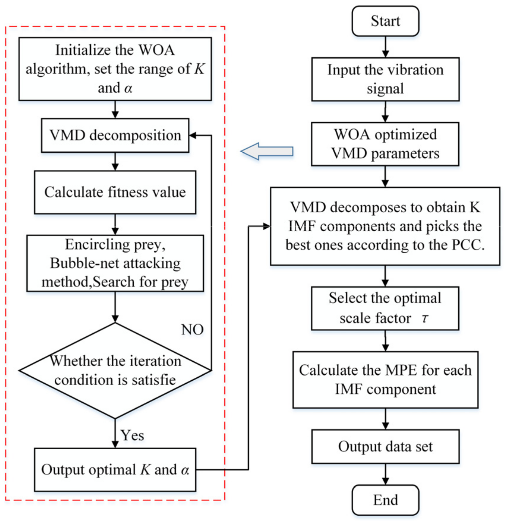
The flow chart of feature extraction based on WOA-VMD and MPE is shown in Figure 1. The specific steps are as follows:
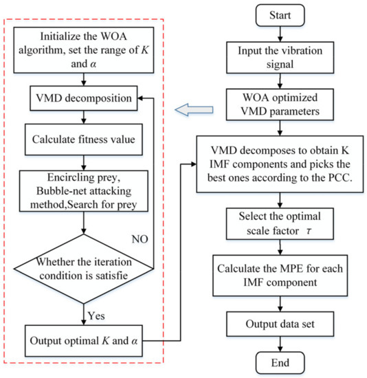
Figure 1.
The flow chart of feature extraction based on WOA-VMD and MPE.
- Step 1. Initialize the WOA algorithm, take the envelope entropy as the fitness function of the WOA, and obtain the global optimal parameters (K, α) for the VMD decomposition of the signal.
- Step 2. VMD decomposition of the vibration signal according to (K, α) obtained in step 1 to obtain K IMF components and pick the best ones according to the PCC criterion.
- Step 3. Select the optimal MPE parameters and calculate the MPE value of each IMF to form the feature data set.
3. Establishment of Fault Diagnosis Model
3.1. MPSO
The particle swarm optimization (PSO) algorithm is a global optimization algorithm with an efficient search function. However, it is easy to fall into the local optimum, the accuracy decreases in the late iteration, and the convergence speed is slow when searching for the best [39], so this paper proposes the improved particle swarm optimization (MPSO) algorithm. MPSO adopts linear decreasing weights and time-varying learning factors to optimize PSO, which improves the search ability and convergence speed of the algorithm. In the MPSO optimization principle, in a D-dimensional vector, the position of the p-th particle is , the velocity is , the optimal position of the particle is , and the optimal position of all particles is .
The velocity and position update equations are as follows:
where is the inertia weight; and are the learning factor constants; and and are uniform random numbers in the range of [0, 1].
The inertia weight represents the ability of the particle to maintain the velocity of motion at the previous moment. When the value of is small, the local search ability is stronger, and when the value of is larger, the global search ability is stronger. In the early stages of the search, the global search ability needs to be improved to avoid getting into local optimal solutions, and in the later stages of the search, the local search ability needs to be improved to find optimal solutions. The linear decreasing inertia weights can better balance the global and local search ability of the algorithm, and the expression is as follows:
where is the maximum value of inertia weight, is the minimum value of inertia weight, is the current number of iterations, and is the maximum number of iterations.
The learning factor represents particle self-awareness and represents particle social awareness. In order to facilitate particle search, it is necessary to improve self-awareness in the early stages of the search and social awareness in the latter stages. The expression of the learning factor is:
where and are the initial and final values of ; and are the initial and final values of and are constants.
3.2. LSSVM Fault Diagnosis Model Based on MPSO Optimization
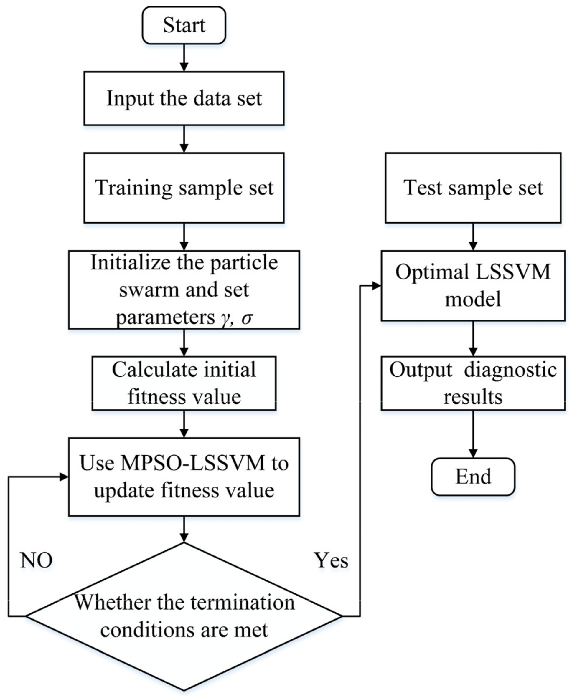
The selection of the regularization parameter γ and the radial basis kernel function parameter σ in the LSSVM model with radial basis function (RBF) as the kernel function is critical when classifying faults in rolling bearings, and the improper selection of the parameters will lead to poor classification model results. The initial value selection in the pre-classification stage is random, and in the past, it relied on experience to select the appropriate parameters, which can cause the problem of underfitting or overfitting to occur. The MPSO algorithm is used to optimize the parameter combination (γ, σ), which avoids the above disadvantages and greatly improves the classification accuracy of the LSSVM model. The specific process is shown in Figure 2.
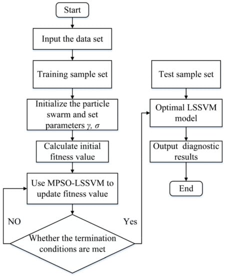
Figure 2.
Flow chart of the MPSO optimized LSSVM model.
The MPSO-LSSVM steps are as follows:
- Step 1: Extract the fault features of rolling bearing vibration signal processing and construct them into a training set and a test set.
- Step 2: Initialize particle swarm parameters. The dimension is two because the parameter combination (γ, σ) is optimized. The parameters of the algorithm are set and the initial swarm of particles is generated randomly.
- Step 3: Calculate the accuracy error of each particle as the fitness value through Equation (20), and the smaller the fitness value, the better the diagnosis result of the LSSVM model. That is:where is the number of correct classifications and is the number of wrong classifications.
- Step 4: According to the particle fitness, the velocity and position of the particle are updated by Equations (16) and (17).
- Step 5: If the maximum number of iterations or the termination condition is satisfied, the loop ends and the optimal combination of parameters is output to construct the MPSO-LSSVM model. Otherwise, return to Step 4.
- Step 6: Input the test set into the constructed MPSO-LSSVM model to obtain the fault diagnosis result.
4. Experiment
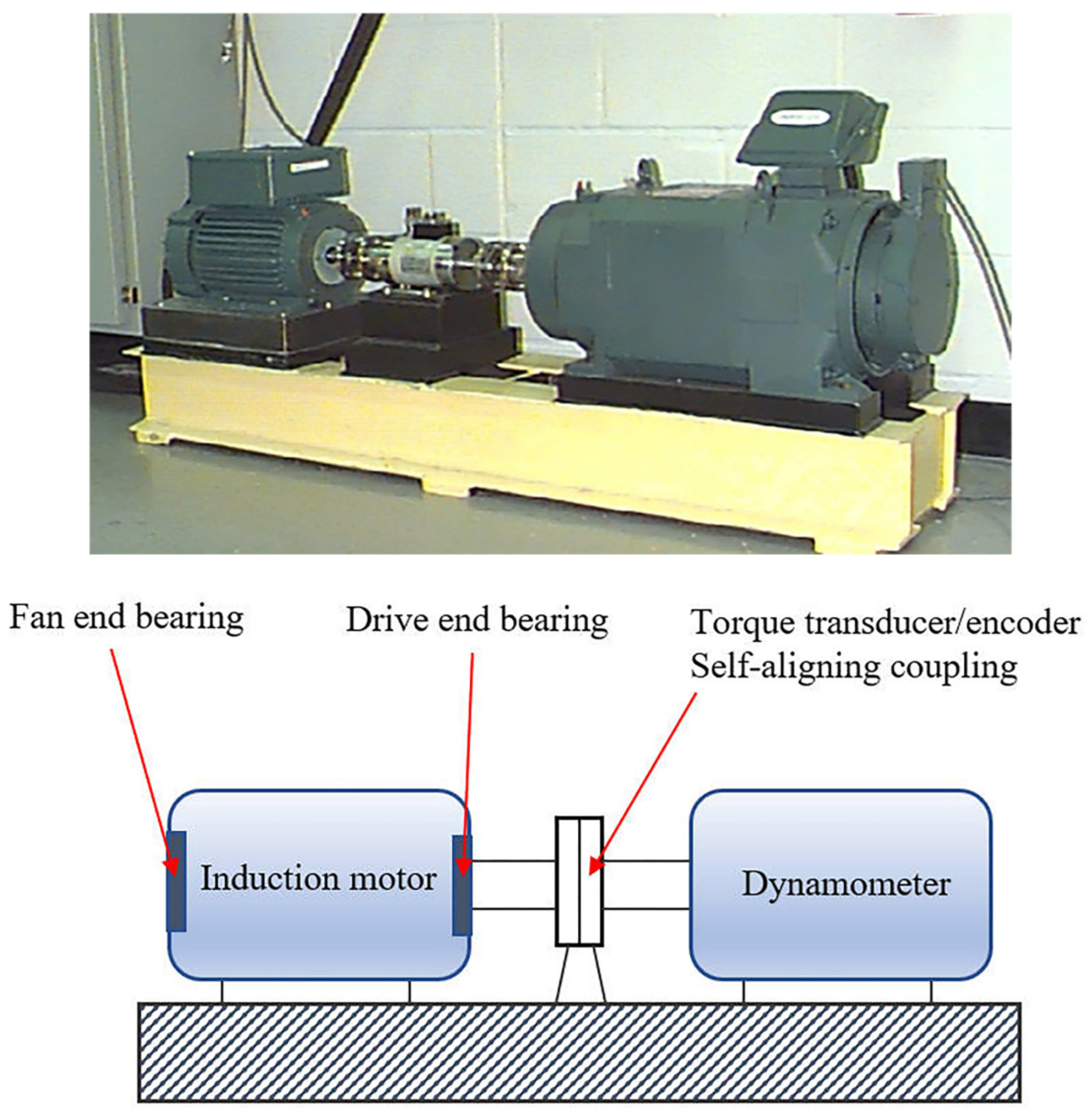
This paper adopts the Western Reserve University bearing test bench data to verify the method [40]. Figure 3 shows a diagram of the experimental setup. The main shaft of the motor is supported by the fan end (FE) and drive end (DE) bearings, respectively, and the bearings are pitted by EDM to simulate common failures. The vibration signals of the drive-side bearing type SKF 6205 2RS acquired by a 16-way DAT recorder with a motor speed of 1797 r/min, a sampling frequency of 12 kHz, and a load of 0 hp are used in the experiments. The vibration signals are collected in four states: the normal (Normal), the inner race fault (IRF), the outer race fault (ORF), and the ball fault (BF). In this study, 100 groups of each state are sampled, and 400 groups of four states are sampled, with 1024 sampling points per group.

Figure 3.
Test device.
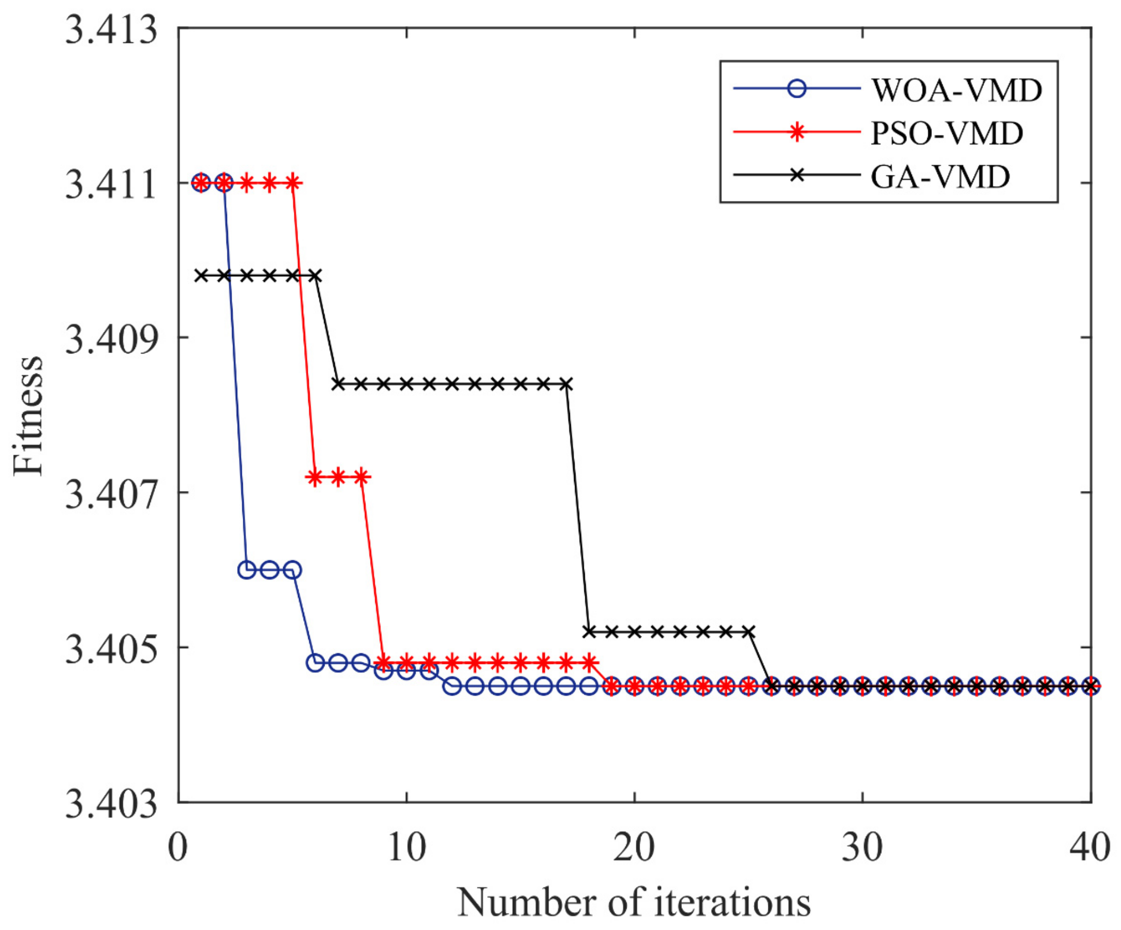
Using the signal of the bearing inner race fault as an example, the WOA algorithm is used to find the optimal parameter combination (K, α) of VMD decomposition. To verify the effectiveness of WOA in VMD parameter optimization, PSO-VMD and GA-VMD are used to compare and verify WOA-VMD, respectively. The initial parameters are as follows: the maximum iteration number is 40, the population size is 20, the average value of 20 tests is taken, the range of K is [2, 10], and the range of α is [500, 6000]. The convergence comparison of the three optimization algorithms is shown in Figure 4.

Figure 4.
Fitness curve of three optimization algorithms.
It can be seen from Figure 4 that PSO-VMD, GA-VMD, and WOA-VMD converge at the 12th, 18th, and 26th generations, respectively, and the convergence value is 3.4045. The convergence speed of the WOA-VMD fitness value optimization curve is the fastest. Table 1 shows the average time taken to run VMD under three optimization algorithms.

Table 1.
Average time required to run VMD under three optimization algorithms.
It can be seen from Table 1 that GA-VMD runs the longest and WOA-VMD runs the shortest. It shows that the WOA-VMD algorithm has advantages over the GA-VMD and PSO-VMD algorithms.
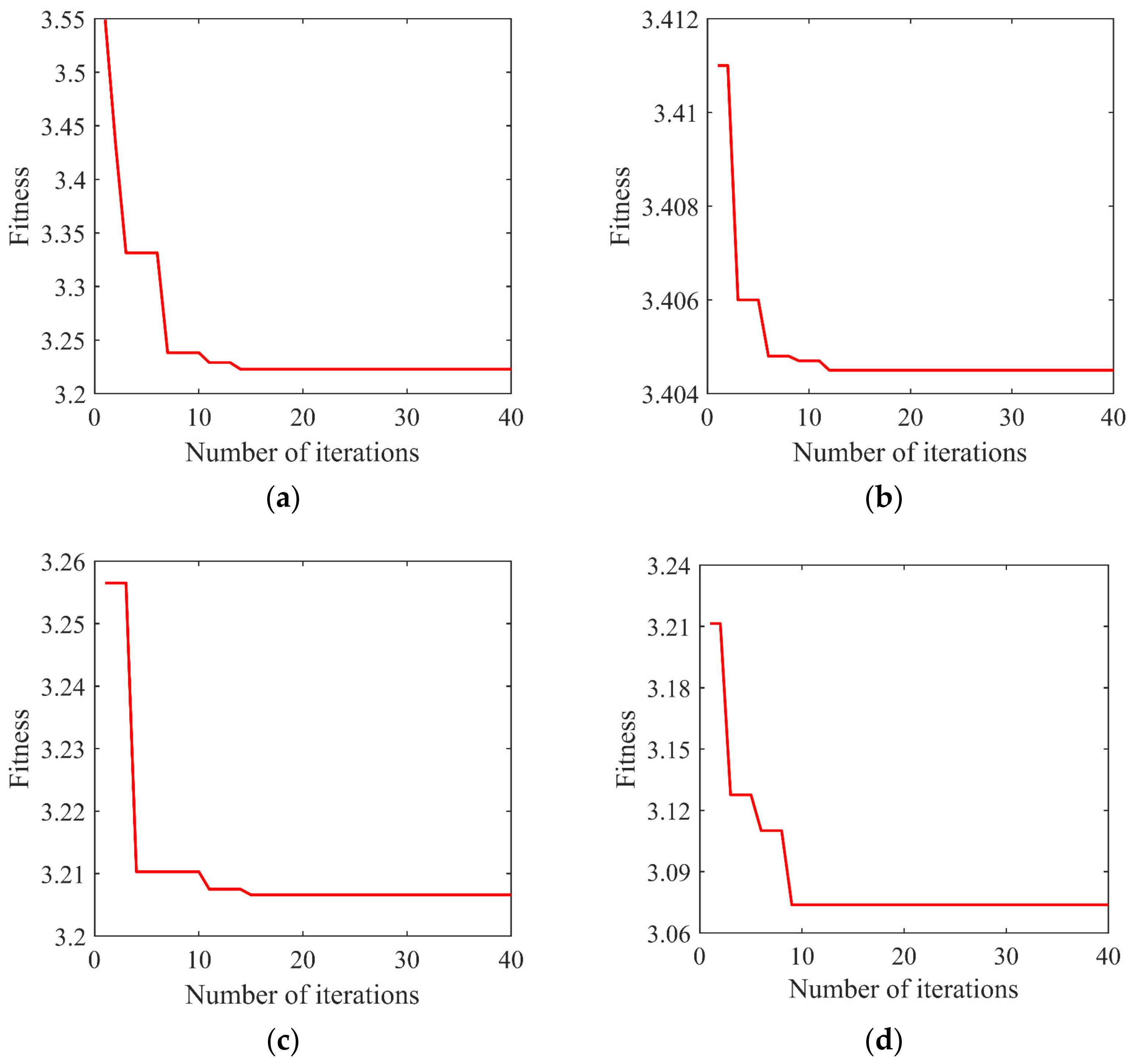
The WOA-VMD optimization algorithm is used to optimize the four bearing signals, and the fitness curve is shown in Figure 5. Figure 5a shows that after 14 iterations, the best fitness of the normal signal is obtained, the convergence value is 3.2228, and the best parameter combination (K, α) is (9, 2103). Figure 5b shows that after 12 iterations, the best fitness of the inner race fault signal is obtained, the convergence value is 3.4045, and the best parameter combination (K, α) is (6, 3648). Figure 5c shows that after 15 iterations, the best fitness of the outer race fault signal is obtained, the convergence value is 3.2066, and the best parameter combination (K, α) is (7, 2585). Figure 5d shows that after nine iterations, the best fitness of the ball fault signal is obtained, the convergence value is 3.0738, and the best parameter combination (K, α) is (9, 3029). The result of the four data optimizations is shown in Table 2.
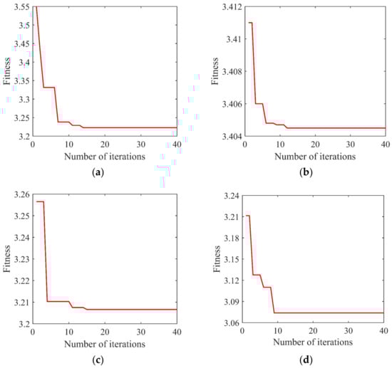
Figure 5.
Fitness curve of the WOA-VMD algorithm: (a) the normal signal; (b) the inner race fault signal; (c) the outer race fault signal; (d) the ball fault signal.
Table 2.
Optimal parameter combination.
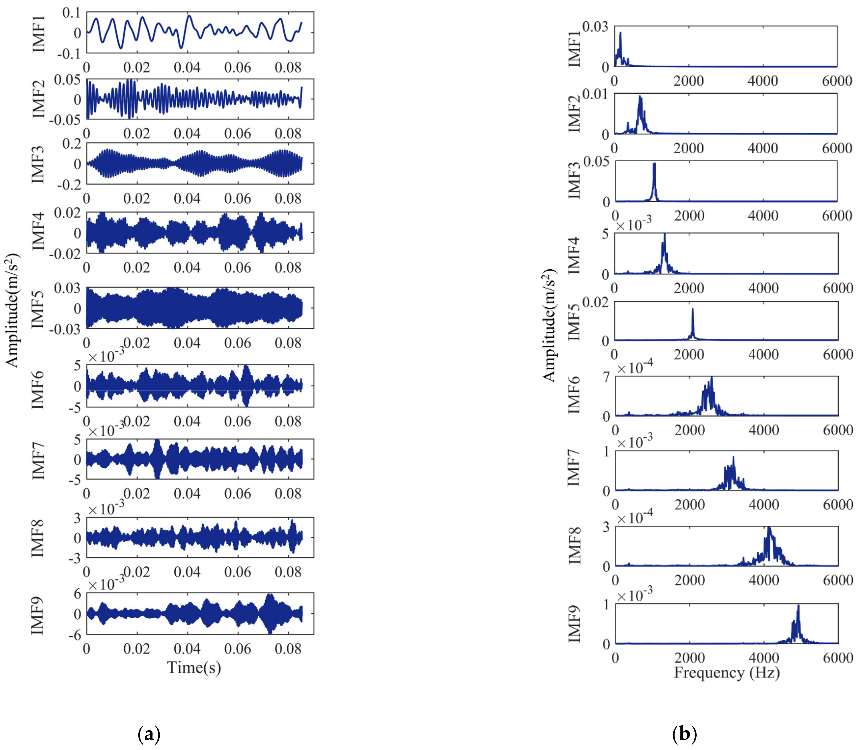
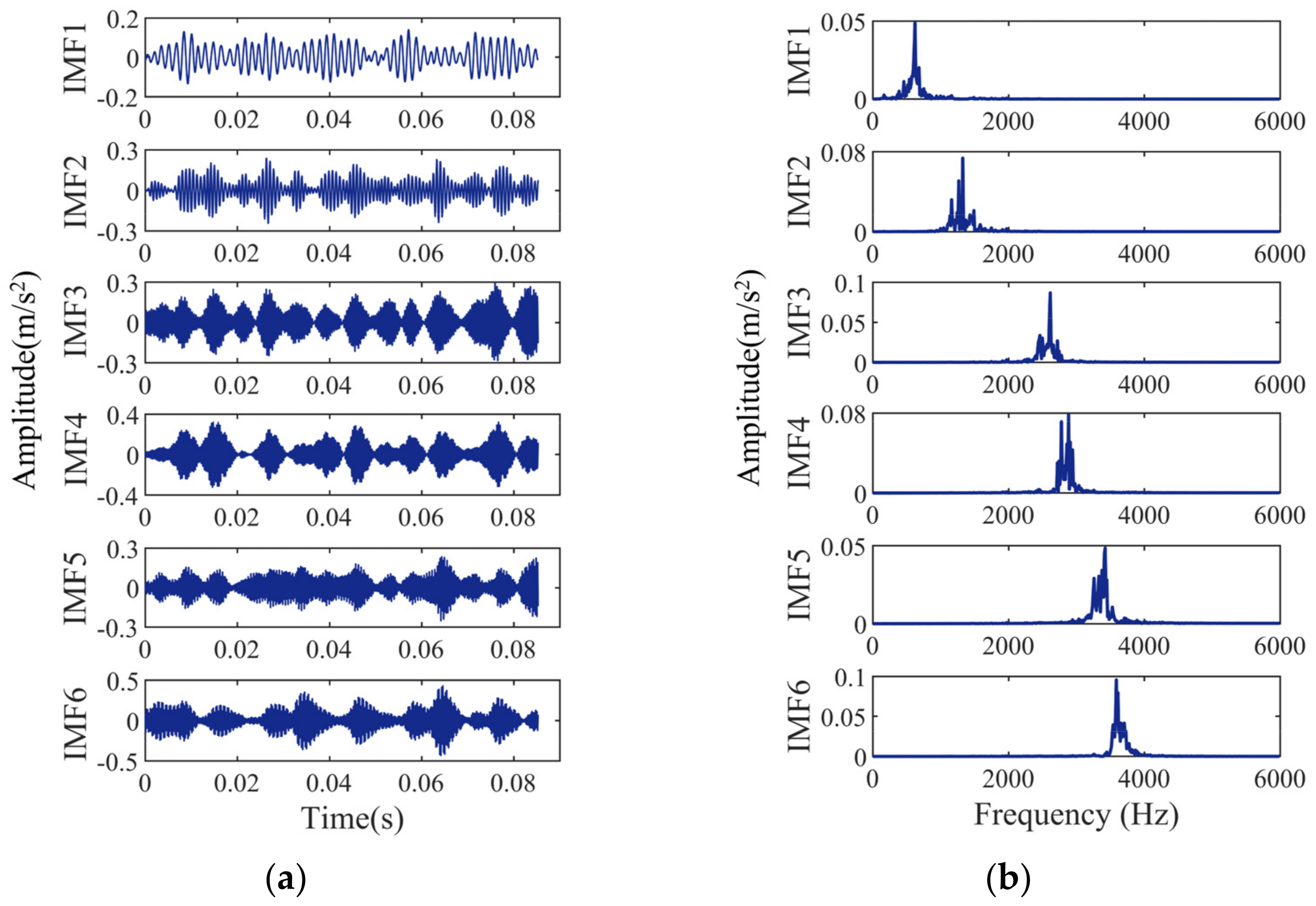
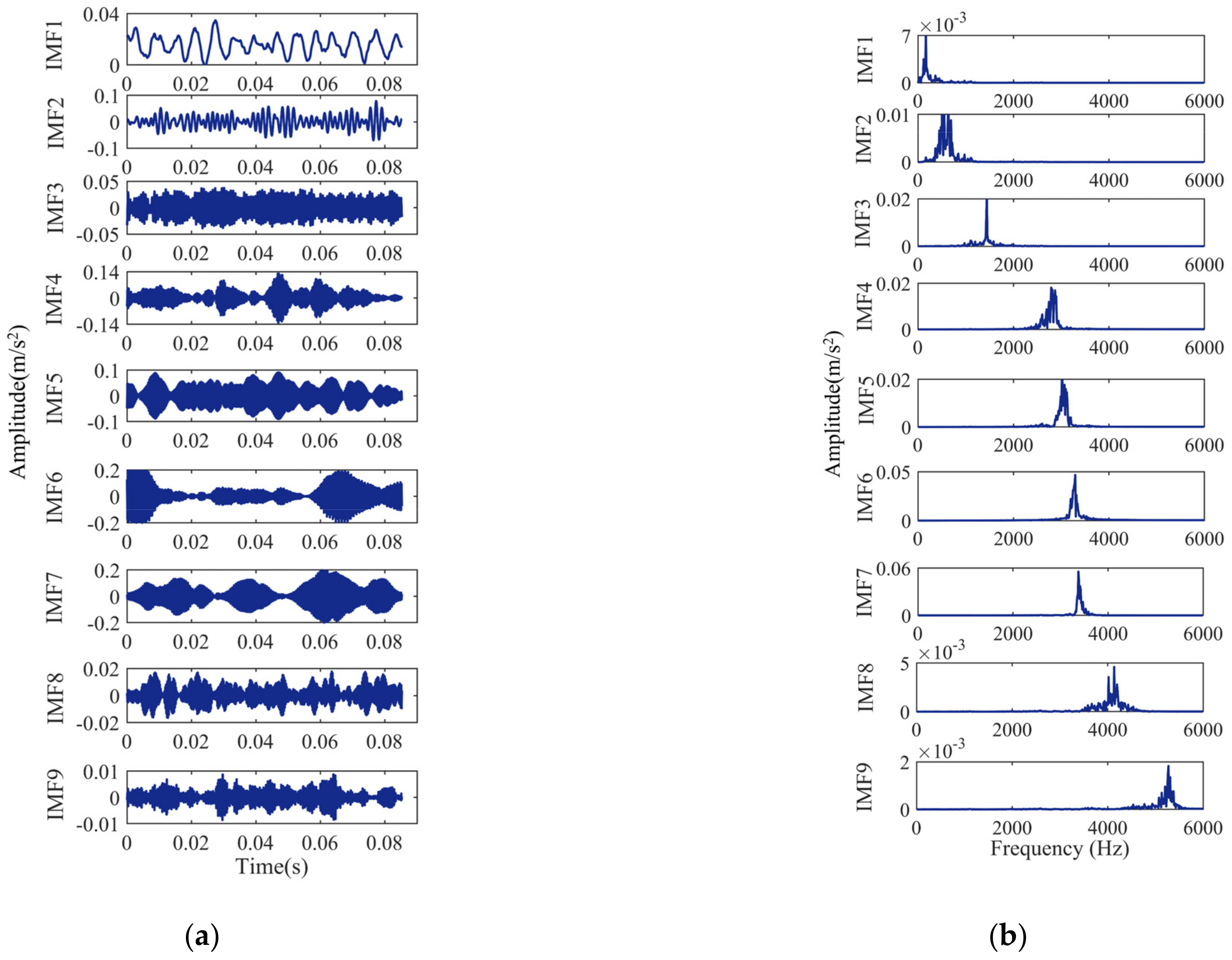
The bearing signals are VMD decomposed, and the decomposition results are shown in Figure 6, Figure 7, Figure 8 and Figure 9. Figure 6a, Figure 7a, Figure 8a and Figure 9a show the time-domain waveform. The frequency-domain analysis is performed on the decomposed IMF, and its frequency spectrum is shown in Figure 6b, Figure 7b, Figure 8b and Figure 9b. It can be seen from Figure 6b, Figure 7b, Figure 8b and Figure 9b that the IMFs have different central frequencies and no defects such as state aliasing and signal distortion, and the original signal can be effectively decomposed.

Figure 6.
Analysis results of the normal signal: (a) the time-domain waveform; (b) frequency spectrum of the IMFs.

Figure 7.
Analysis results of the inner race fault signal: (a) the time-domain waveform; (b) frequency spectrum of the IMFs.
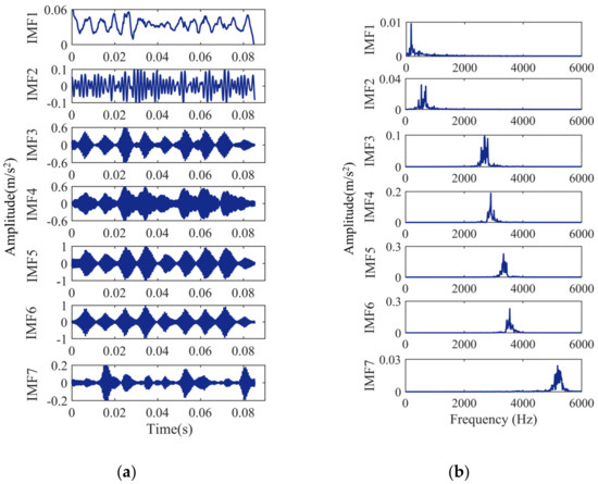
Figure 8.
Analysis results of the outer race fault signal: (a) the time-domain waveform; (b) frequency spectrum of the IMFs.

Figure 9.
Analysis results of the ball fault signal: (a) the time-domain waveform; (b) frequency spectrum of the IMFs.
According to the PCC, the Pearson correlation coefficients between each IMF and the original signal are calculated. The calculated results are shown in Table 3, Table 4, Table 5 and Table 6.
Table 3.
PCC values of the normal (Normal) signal’s various IMF components.
Table 4.
PCC values of the outer race fault (ORF) signal’s various IMF components.
Table 5.
PCC values of the ball fault (BF) signal’s various IMF components.
Table 6.
PCC values of the inner race fault (IRF) signal’s various IMF components.
It can be seen from Table 3 that the components of IMF1, IMF2, IMF3, and IMF5 obtained by VMD decomposition of the normal (Normal) signal meet the PCC condition with a correlation value greater than 0.3. This indicates that IMF1, IMF2, IMF3, and IMF5 components are highly correlated with the original signal, and the signal contains abundant fault information. Therefore, IMF1, IMF2, IMF3, and IMF5 components are selected as the key components. It can be seen from Table 4 that the IMF3, IMF4, IMF5, and IMF6 components obtained by VMD decomposition of the outer race fault (ORF) signal meet the PCC condition with correlation values greater than 0.3. Therefore, IMF3, IMF4, IMF5, and IMF6 components are selected as the key components. It can be seen from Table 5 that the IMF4, IMF5, IMF6, and IMF7 components obtained by VMD decomposition of the ball fault (BF) signal meet the PCC condition with a correlation value greater than 0.3. Therefore, IMF4, IMF5, IMF6, and IMF7 components are selected as the key components. It can be seen from Table 6 that the components of IMF2, IMF3, IMF4, IMF5, and IMF6 obtained by VMD decomposition of the inner race fault (IRF) signal meet the PCC condition with a correlation value greater than 0.3. According to the above analysis, the normal (Normal) signal, the outer race fault (ORF) signal, and the ball fault (BF) signal only have four IMF components that satisfy the PCC condition. Therefore, in order to ensure the same dimension of the eigenvectors obtained below, the IMF3, IMF4, IMF5, and IMF6 components are selected as optimal components. A new array can be formed based on the order of the optimal IMF components obtained above. The result is shown in Table 7.
Table 7.
The array of four optimal IMF components of bearing signals.
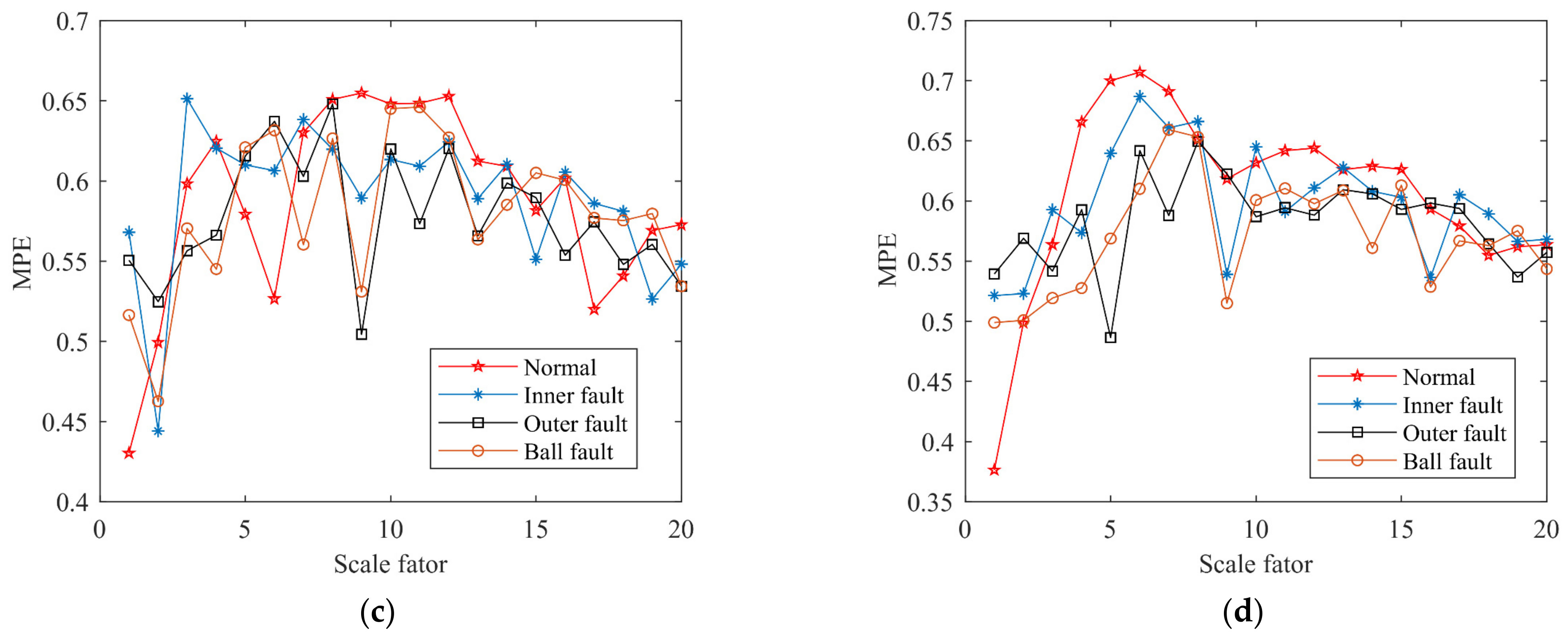
The selection of MPE parameters is extremely important and determines the accuracy of fault diagnosis. The method of determining the optimal MPE parameters is introduced, initially setting the embedding dimension s = 6, the delay time t = 1, and setting the scale factor to τ = 20. Figure 10 shows the relationship between MPE values of the array U and scale factor τ. It can be seen from Figure 10a that when τ = 2, the difference in MPE value is larger, and four states can be clearly distinguished. Therefore, the value of the optimal scale factor for U1 is determined as 2 and uses the same method to determine the optimal scale factor τ = 4, τ = 9, and τ = 5 of U2, U3, and U4. The result is shown in Table 8.
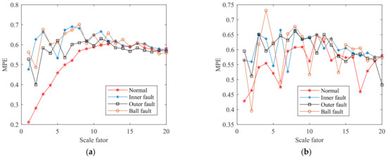
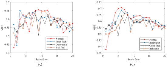
Figure 10.
Relationship curve between MPE values of the array U and scale factor τ: (a) the array U1; (b) the array U2; (c) the array U3; (d) the array U4.
Table 8.
The optimal scale factor τ of each U component.
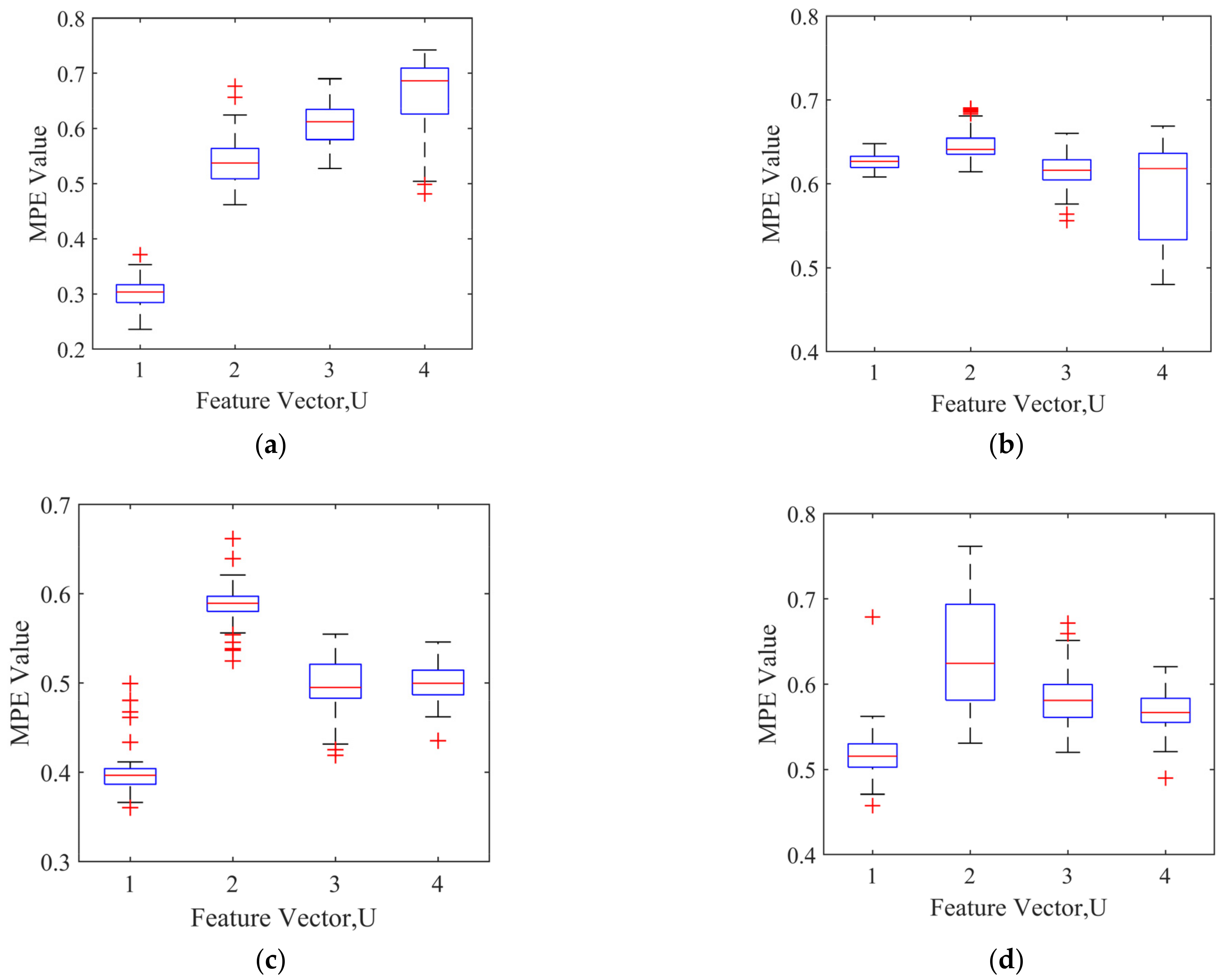
According to the optimal scale factor τ, the optimal MPE is selected to form the feature vectors. The feature vectors in the four states are normalized to the range of (0, 1) to form the feature vector data set, for which Table 9 shows the feature vector data set. Figure 11 is the boxplot of the feature vector U for the four types of bearing signals. It can be seen from Figure 11 that the feature vectors are relatively concentrated.
Table 9.
Feature vector data set.
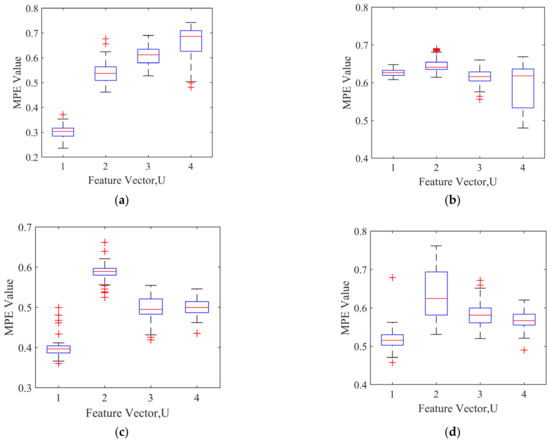
Figure 11.
The boxplot of the feature vector U: (a) the normal feature vector boxplot; (b) the inner race fault feature vector boxplot; (c) the outer race fault feature vector boxplot; (d) the ball fault feature vector boxplot.
5. Analysis of Fault Diagnosis Results
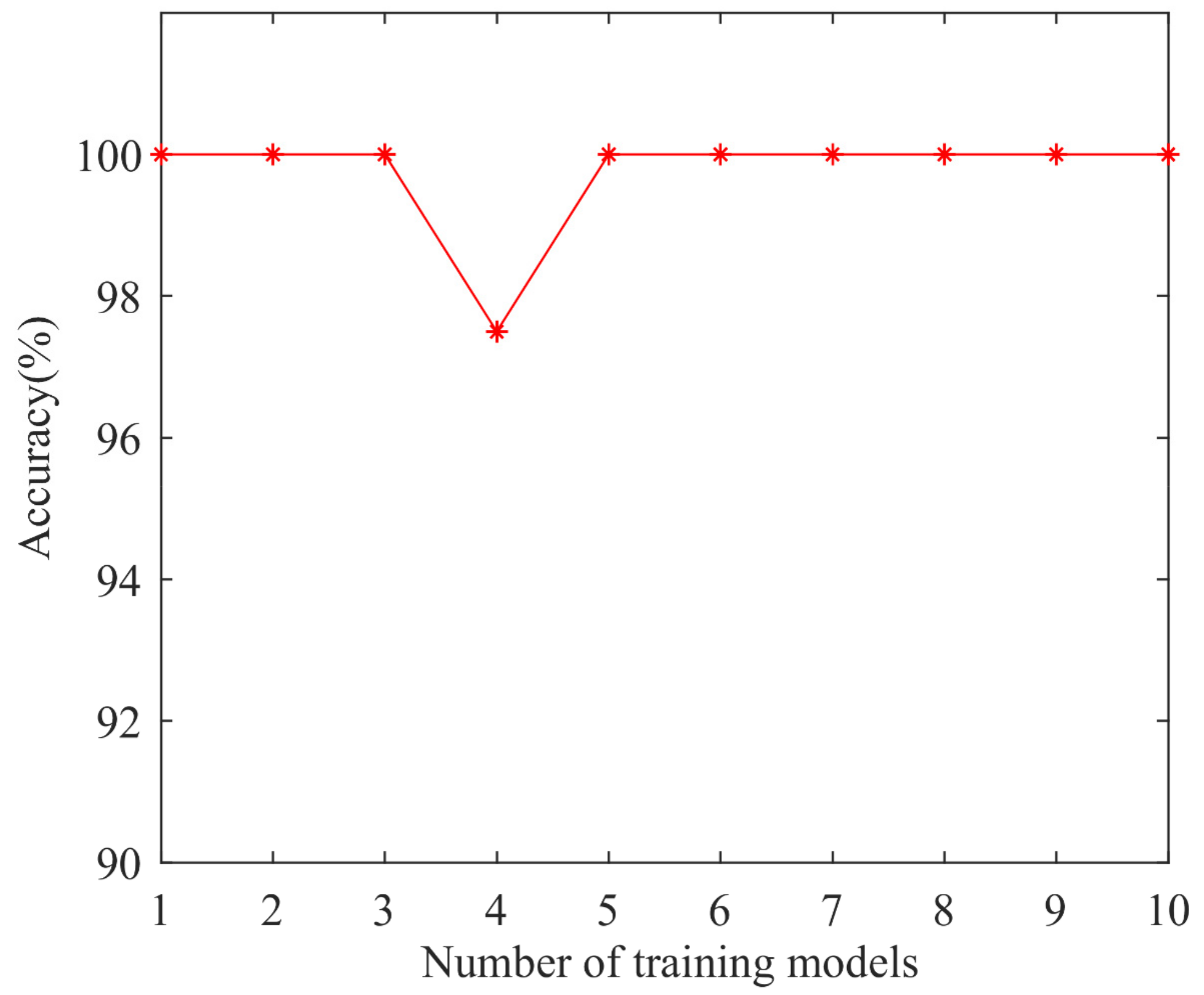
The feature vector data set is input into the LSSVM model for classification, and the MPSO algorithm is used to optimize the model. The parameters of the MPSO-LSSVM algorithm are set as follows: the , , , and values are 2, 1, 1, 2, the is 0.9, the is 0.1, the number of particles is 30, the number of iterations is 200, the penalty factor range is [0.1, 100], and the radial basis kernel parameter range is [0.1, 100]. For the multi-classification problem, the sample data is grouped and trained by the K-fold cross-validation method. K = 10 is selected, each subset of data is used as a validation set, and the remaining nine sets of subset data are combined as a training set, which is brought into the MPSO-LSSVM model for training. The accuracy rate of 10 groups of discriminant models obtained through training is shown in Figure 12, and the average accuracy is 99.75%, which proves that the model can perfectly discriminate the fault types of rolling bearings and effectively avoid the effects of over-fitting.
Figure 12.
The accuracy of the discriminant model.
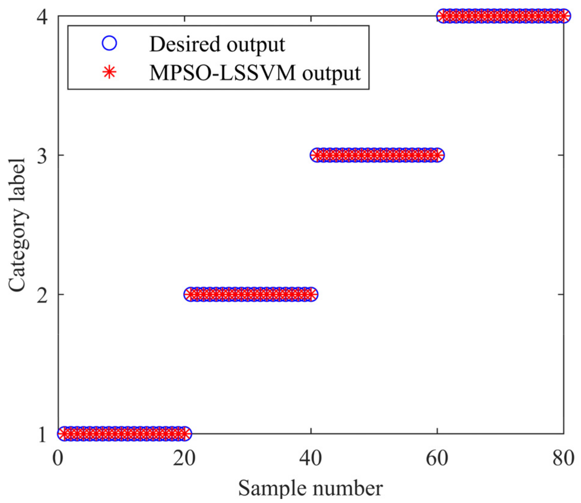
In order to verify whether the model trained by K-fold cross-validation has excellent generalization ability, a total of 80 test samples are classified and identified by taking 20 test samples of the normal, inner race fault, outer race fault, and ball fault. The fitness curve of the algorithm with the number of iterations is shown in Figure 13. The MPSO algorithm optimizes the optimal combination of LSSVM parameters (γ, σ) as (30.65, 7.13), and the accuracy of the model is 99.88%. The classification result is shown in Figure 14. It can be seen from Figure 14 that the classification rate is 100%.
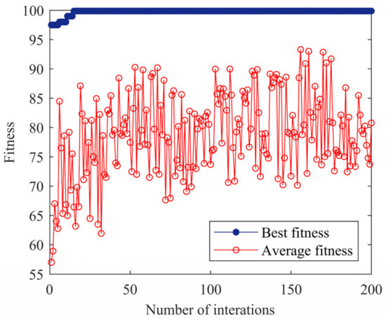
Figure 13.
Fitness curve of the MPSO-LSSVM algorithm.
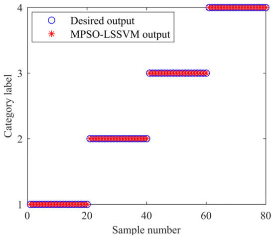
Figure 14.
Classification results of MPSO-LSSVM.
In order to prevent the contingency of experimental results, the test set is tested 20 times and takes an average of 20 results. Table 10 shows the diagnosis results. As can be seen from Table 10, the average accuracy is 100% after optimizing the LSSVM model with the MPSO algorithm, which proves that the MPSO-LSSVM pattern recognition has a strong adaptive capability.
Table 10.
Diagnostic results of the MPSO-LSSVM.
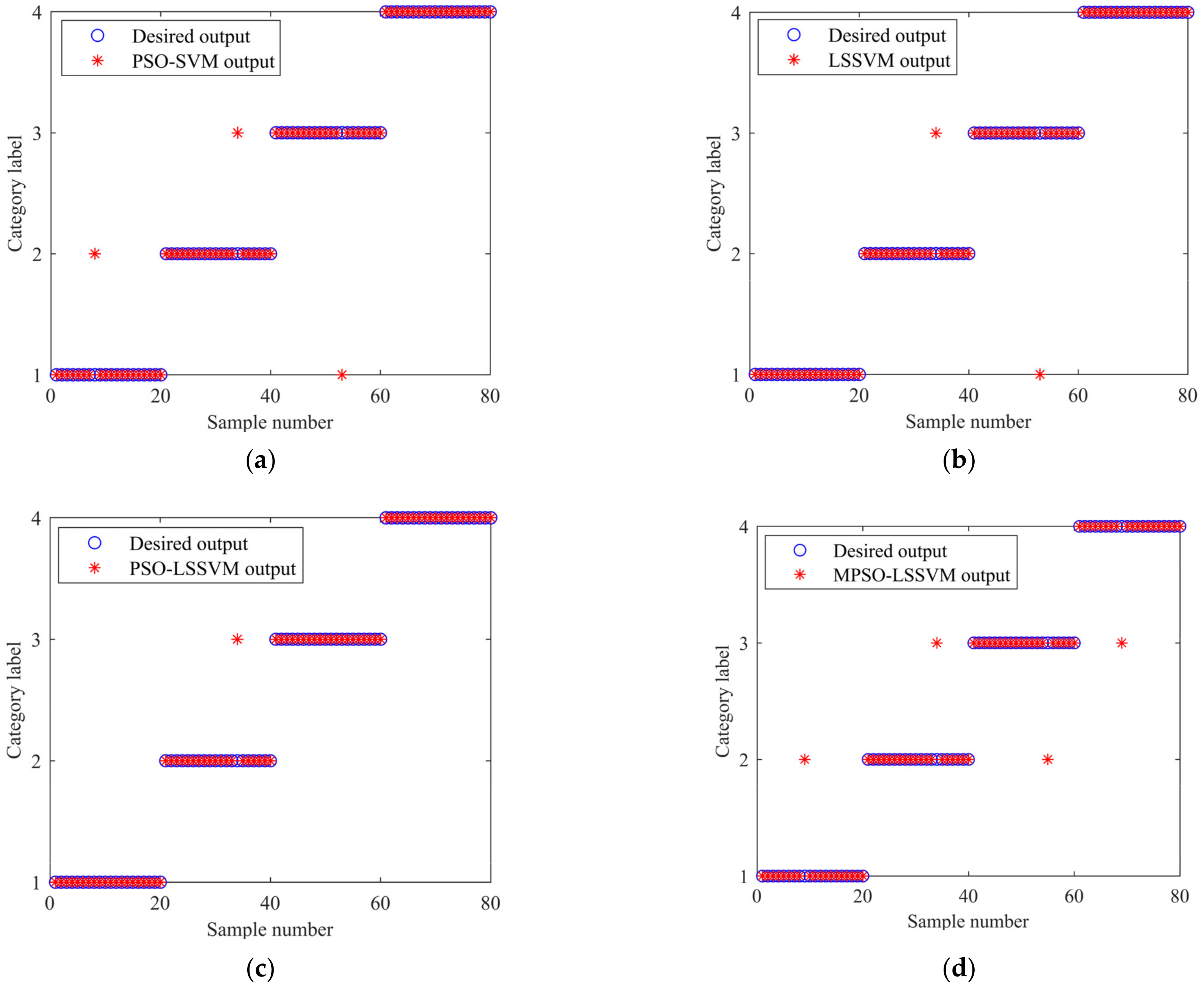
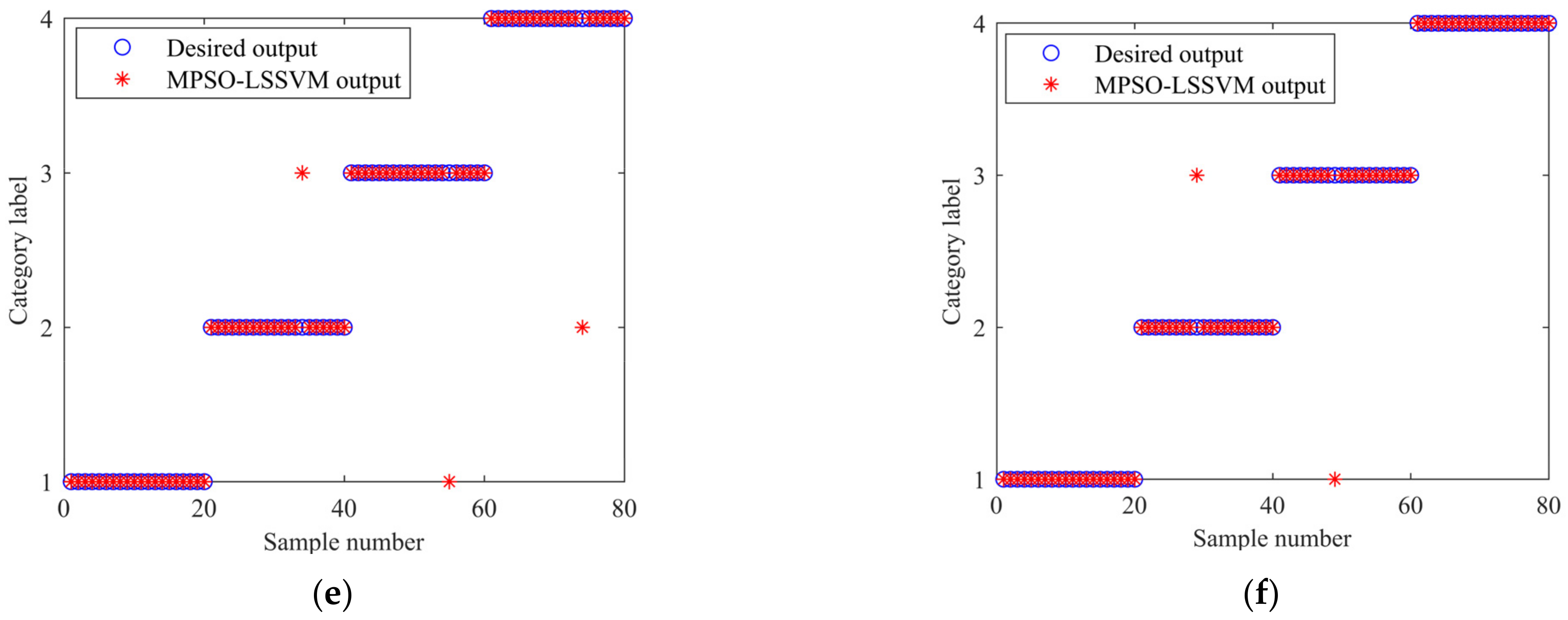
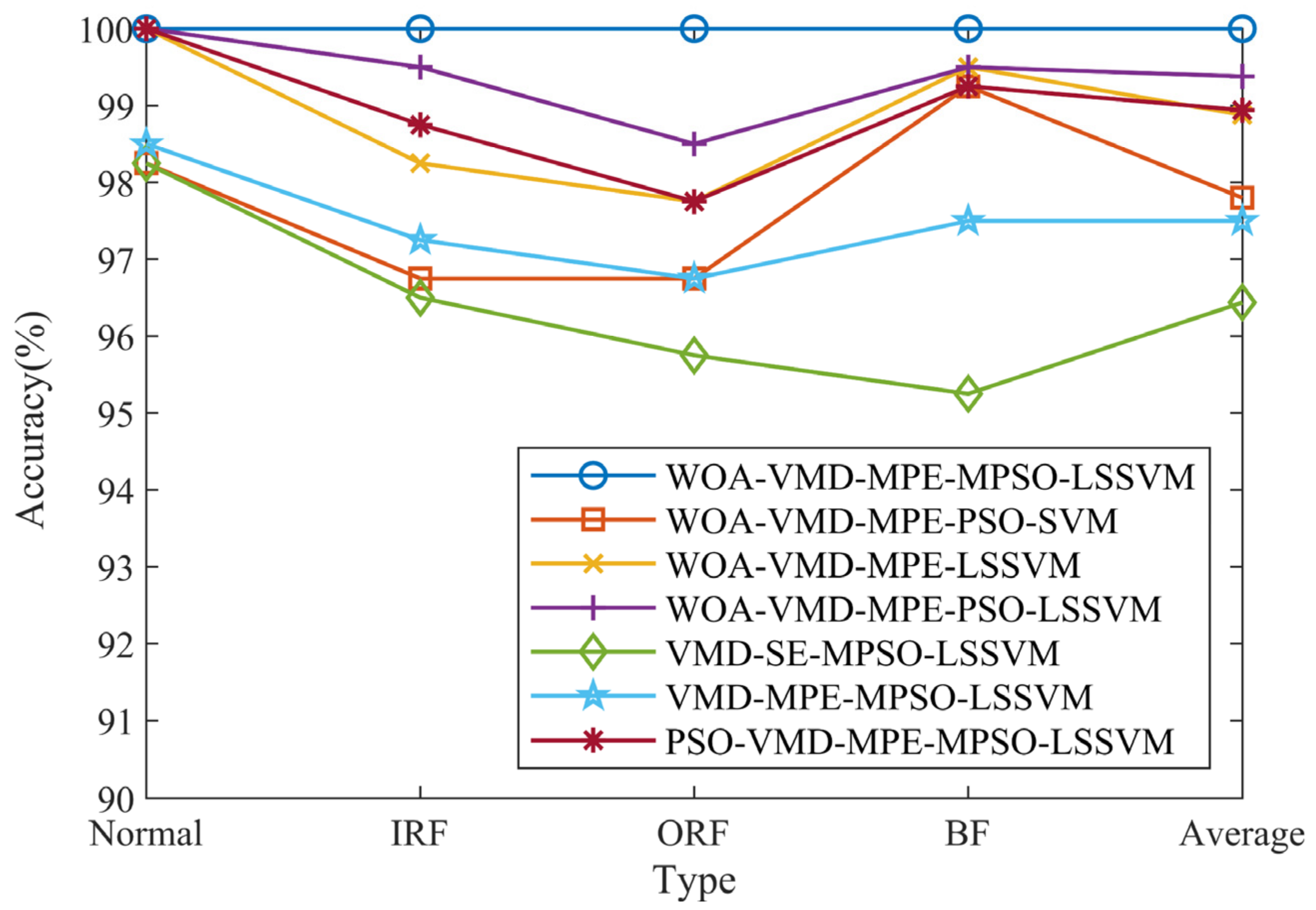
To further verify the superiority of this model, the same bearing faults are diagnosed by combining the feature vectors constructed by WOA-VMD-MPE using PSO-SVM, LSSVM, and PSO-LSSVM, respectively. Meanwhile, the feature vectors constructed by VMD-SE, VMD-MPE, and PSO-VMD-MPE are combined with the MPSO-LSSVM model for fault identification to verify the effectiveness of the features extracted by WOA-VMD-MPE. The classification results are shown in Figure 15. The different methods are tested 20 times to obtain the average value. The specific diagnosis result is shown in Table 11. Figure 16 shows the identification results of different methods. It can be seen from Figure 16 that the method of WOA-VMD-MPE-MPSO-LSSVM presented in this paper has the highest accuracy, while the method of VMD-SE-MPSO-LSSVM has the lowest accuracy.
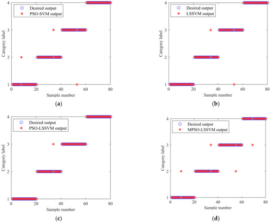
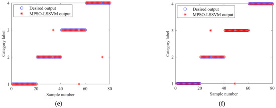
Figure 15.
Classification results: (a) PSO-SVM results with WOA-VMD-MPE; (b) LSSVM results with WOA-VMD-MPE; (c) PSO-LSSVM results with WOA-VMD-MPE; (d) MPSO-LSSVM results with VMD-SE; (e) MPSO-LSSVM results with VMD-MPE; (f) MPSO-LSSVM results with PSO-VMD-MPE.
Table 11.
Diagnostic results of different methods.
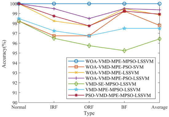
Figure 16.
The identification results of different methods.
From Table 11, it can be seen that the accuracy of PSO-SVM, LSSVM, and PSO-LSSVM models to identify the feature vectors constructed by WOA-VMD-MPE is 97.80%, 98.88%, and 99.38%, respectively, which is lower than the method proposed in this paper. The identification accuracy of the MPSO-LSSVM model to identify the feature vectors constructed by VMD-SE, VMD-MPE, and PSO-VMD-MPE is 96.44%, 97.50%, and 98.94%, respectively, which is lower than that of WOA-VMD-MPE. Through the above analysis, the effectiveness of the MPSO-LSSVM fault diagnosis method based on the combination of WOA-VMD-MPE is verified.
6. Conclusions
A fault diagnosis method based on the modified particle swarm optimization (MPSO) algorithm optimized least square support vector machine (LSSVM) combining parameter optimization variational mode decomposition (VMD) and multi-scale permutation entropy (MPE) is proposed in this paper. The main conclusions are as follows:
- (1)
- The whale optimization algorithm (WOA) is used to optimize the penalty factor α and the number of mode components K in the VMD algorithm so as to solve the problems of insufficient decomposition and mode mixing caused by the improper selection of mode components K and penalty factor α in the VMD algorithm.
- (2)
- In order to extract fault features more accurately, the Pearson correlation coefficient (PCC) criterion is introduced to screen out the optimal IMF, and the multi-scale permutation entropy of the optimal IMF is calculated to form a feature vector. Experimental results show that the WOA-VMD-MPE extracts more accurate features compared to VMD-SE, VMD-MPE, and PSO-VMD-MPE methods.
- (3)
- In order to improve the generalization ability of the MPSO-LSSVM model, K-fold cross-validation is performed on the model, and the average accuracy of the model can reach 99.75%. The test samples are input into the model for classification to verify whether the model has good generalization ability. The results show that the accuracy of fault identification of rolling bearings is 100%. Meanwhile, compared with PSO-SVM, LSSVM, and PSO-LSSVM methods, the MPSO-LSSVM fault diagnosis model has higher identification accuracy.
The improvement needed in this scheme is that the uncertainty in data acquisition is not considered, and there may be some parts of the vibration data that are not collected and can be improved by the acoustic emission technique.
Author Contributions
Conceptualization, methodology, software, writing—original draft, writing—review and editing, G.C.; Funding acquisition, software, proofreading, supervision, Z.J. and Z.Y.; Project administration, resources, Z.J. and Z.Y. All authors have read and agreed to the published version of the manuscript.
Funding
This research was supported by the National Natural Science Foundation of China (No. 11702178), National Natural Science Foundation of China-Liaoning Provincial People’s Government Joint Fund (No. U1708254), Liaoning Doctoral Start-up Fund Grant (No. 20180540013), and Liaoning Education Department Grant (No. LQ2019008).
Institutional Review Board Statement
Not applicable.
Informed Consent Statement
Not applicable.
Data Availability Statement
Data sharing not applicable.
Acknowledgments
The authors would like to thank the anonymous reviewers and the editor for their valuable and insightful suggestions.
Conflicts of Interest
The authors declare no conflict of interest.
References
- Fathiah Waziralilah, N.; Abu, A.; Lim, M.H.; Quen, L.K.; Elfakharany, A. Bearing Fault Diagnosis Employing Gabor and Augmented Architecture of Convolutional Neural Network. J. Mech. Eng. Sci. 2019, 13, 5689–5702. [Google Scholar] [CrossRef]
- Ibarra-Zarate, D.; Tamayo-Pazos, O.; Vallejo-Guevara, A. Bearing Fault Diagnosis in Rotating Machinery Based on Cepstrum Pre-Whitening of Vibration and Acoustic Emission. Int. J. Adv. Manuf. Technol. 2019, 104, 4155–4168. [Google Scholar] [CrossRef]
- Attoui, I.; Oudjani, B.; Boutasseta, N.; Fergani, N.; Bouakkaz, M.S.; Bouraiou, A. Novel Predictive Features Using a Wrapper Model for Rolling Bearing Fault Diagnosis Based on Vibration Signal Analysis. Int. J. Adv. Manuf. Technol. 2020, 106, 3409–3435. [Google Scholar] [CrossRef]
- Zhang, K.; Ma, C.; Xu, Y.; Chen, P.; Du, J. Feature Extraction Method Based on Adaptive and Concise Empirical Wavelet Transform and Its Applications in Bearing Fault Diagnosis. Meas. J. Int. Meas. Confed. 2021, 172, 108976. [Google Scholar] [CrossRef]
- Dragomiretskiy, K.; Zosso, D. Variational Mode Decomposition. IEEE Trans. Signal Process. 2014, 62, 531–544. [Google Scholar] [CrossRef]
- Ram, R.; Mohanty, M.N. Comparative Analysis of EMD and VMD Algorithm in Speech Enhancement. Int. J. Nat. Comput. Res. 2017, 6, 17–35. [Google Scholar] [CrossRef]
- Zhou, Y.; Zhang, Y.; Yang, D.; Lu, J.; Dong, H.; Li, G. Pipeline Signal Feature Extraction with Improved VMD and Multi-Feature Fusion. Syst. Sci. Control Eng. 2020, 8, 318–327. [Google Scholar] [CrossRef]
- Zhang, Y.; Wang, A. Research on the Fault Diagnosis Method for Rolling Bearings Based on Improved VMD and Automatic IMF Acquisition. Shock Vib. 2020, 2020, 6216903. [Google Scholar] [CrossRef]
- Wang, J.; Zhan, C.; Li, S.; Zhao, Q.; Liu, J.; Xie, Z. Adaptive Variational Mode Decomposition Based on Archimedes Optimization Algorithm and Its Application to Bearing Fault Diagnosis. Measurement 2022, 191, 110798. [Google Scholar] [CrossRef]
- Jiao, J.; Yue, J.; Pei, D. Feature Enhancement Method of Rolling Bearing Based on K-Adaptive VMD and RBF-Fuzzy Entropy. Entropy 2022, 24, 197. [Google Scholar] [CrossRef]
- Duan, J.; Wang, P.; Ma, W.; Tian, X.; Fang, S.; Cheng, Y.; Chang, Y.; Liu, H. Short-Term Wind Power Forecasting Using the Hybrid Model of Improved Variational Mode Decomposition and Correntropy Long Short-Term Memory Neural Network. Energy 2021, 214, 118980. [Google Scholar] [CrossRef]
- Li, Y.; Tang, B.; Jiang, X.; Yi, Y. Bearing Fault Feature Extraction Method Based on GA-VMD and Center Frequency. Math. Probl. Eng. 2022, 2022, 2058258. [Google Scholar] [CrossRef]
- He, D.; Liu, C.; Jin, Z.; Ma, R.; Chen, Y.; Shan, S. Fault Diagnosis of Flywheel Bearing Based on Parameter Optimization Variational Mode Decomposition Energy Entropy and Deep Learning. Energy 2022, 239, 122108. [Google Scholar] [CrossRef]
- Xue, Q.; Xu, B.; He, C.; Liu, F.; Ju, B.; Lu, S.; Liu, Y. Feature Extraction Using Hierarchical Dispersion Entropy for Rolling Bearing Fault Diagnosis. IEEE Trans. Instrum. Meas. 2021, 70, 3521311. [Google Scholar] [CrossRef]
- Wang, H.; Du, W.; Li, H.; Li, Z.; Hu, J. Weak Fault Feature Extraction of Rolling Element Bearing Based on Variational Mode Extraction and Multi-Objective Information Fusion Band-Pass Filter. J. Vibroeng. 2021, 24, 30–45. [Google Scholar] [CrossRef]
- Yang, J.; Wu, C.; Shan, Z.; Liu, H.; Yang, C. Extraction and Enhancement of Unknown Bearing Fault Feature in the Strong Noise under Variable Speed Condition. Meas. Sci. Technol. 2021, 32, 105021. [Google Scholar] [CrossRef]
- Yan, X.; Xu, Y.; She, D.; Zhang, W. A Bearing Fault Diagnosis Method Based on PAVME and MEDE. Entropy 2021, 23, 1402. [Google Scholar] [CrossRef]
- Zheng, X.; Zhou, G.; Li, D.; Zhou, R.; Ren, H. Application of Variational Mode Decomposition and Permutation Entropy for Rolling Bearing Fault Diagnosis. Int. J. Acoust. Vib. 2019, 24, 303–311. [Google Scholar] [CrossRef]
- Zhang, J.; Zhang, J.; Zhong, M.; Zheng, J.; Yao, L. A GOA-MSVM Based Strategy to Achieve High Fault Identification Accuracy for Rotating Machinery under Different Load Conditions. Measurement 2020, 163, 108067. [Google Scholar] [CrossRef]
- Vapnik, V.N. The Nature of Statistical Learning Theory; Springer: New York, NY, USA, 1995. [Google Scholar] [CrossRef]
- Zhang, Q.; Chen, S.; Fan, Z.P. Bearing Fault Diagnosis Based on Improved Particle Swarm Optimized VMD and SVM Models. Adv. Mech. Eng. 2021, 13, 1–12. [Google Scholar] [CrossRef]
- Wang, Y.; Xu, C.; Wang, Y.; Cheng, X.; Fusco, G.; Zhu, Q.; Na, J.; Zhang, W.; Azar, A.T. A Comprehensive Diagnosis Method of Rolling Bearing Fault Based on CEEMDAN-DFA-Improved Wavelet Threshold Function and QPSO-MPE-SVM. Entropy 2021, 23, 1142. [Google Scholar] [CrossRef] [PubMed]
- Ye, M.; Yan, X.; Jia, M. Rolling Bearing Fault Diagnosis Based on VMD-MPE and PSO-SVM. Entropy 2021, 23, 762. [Google Scholar] [CrossRef] [PubMed]
- Suykens, J.A.K.; Vandewalle, J. Least Squares Support Vector Machine Classifiers. Neural Process. Lett. 1999, 9, 293–300. [Google Scholar] [CrossRef]
- Li, Y.; Huang, D.; Qin, Z. A Classification Algorithm of Fault Modes-Integrated LSSVM and PSO with Parameters’ Optimization of VMD. Math. Probl. Eng. 2021, 2021, 6627367. [Google Scholar] [CrossRef]
- Li, Y.; Yang, P.; Wang, H. Short-Term Wind Speed Forecasting Based on Improved Ant Colony Algorithm for LSSVM. Clust. Comput. 2018, 22, 11575–11581. [Google Scholar] [CrossRef]
- Gao, X.; Wei, H.; Li, T.; Yang, G. A Rolling Bearing Fault Diagnosis Method Based on LSSVM. Adv. Mech. Eng. 2014, 12, 1687814019899561. [Google Scholar] [CrossRef]
- Yousefi, M.; Gholami, M.; Oskoei, V.; Mohammadi, A.A.; Baziar, M.; Esrafili, A. Comparison of LSSVM and RSM in Simulating the Removal of Ciprofloxacin from Aqueous Solutions Using Magnetization of Functionalized Multi-Walled Carbon Nanotubes: Process Optimization Using GA and RSM Techniques. J. Environ. Chem. Eng. 2021, 9, 105677. [Google Scholar] [CrossRef]
- He, D.; Lu, K.; Xiao, Q. Power Electronic Circuits Fault Diagnosis Based on Wavelet Packet Transform and LSSVM. J. Meas. Eng. 2017, 5, 68–76. [Google Scholar] [CrossRef] [Green Version]
- Gao, S.; Li, T.; Zhang, Y. Rolling Bearing Fault Diagnosis of PSO-LSSVM Based on CEEMD Entropy Fusion. Trans. Can. Soc. Mech. Eng. 2020, 44, 405–418. [Google Scholar] [CrossRef]
- Zhao, X.; Qin, Y.; He, C.; Jia, L. Intelligent Fault Identification for Rolling Element Bearings in Impulsive Noise Environments Based on Cyclic Correntropy Spectra and LSSVM. IEEE Access 2020, 8, 40925–40938. [Google Scholar] [CrossRef]
- Zhu, X.; Huang, Z.; Chen, J.; Lu, J. Rolling Bearing Fault Diagnosis Method Based on VMD and LSSVM. J. Phys. Conf. Ser. 2021, 1792, 012035. [Google Scholar] [CrossRef]
- An, G.; Tong, Q.; Zhang, Y.; Liu, R.; Li, W.; Cao, J.; Lin, Y.; Wang, Q.; Zhu, Y.; Pu, X. A Parameter-Optimized Variational Mode Decomposition Investigation for Fault Feature Extraction of Rolling Element Bearings. Math. Probl. Eng. 2021, 2021, 6629474. [Google Scholar] [CrossRef]
- Benesty, J.; Chen, J.; Huang, Y.; Cohen, I. Pearson Correlation Coefficient. In Noise Reduction in Speech Processing; Springer Topics in Signal Processing; 2009; Volume 2, pp. 1–4. [Google Scholar] [CrossRef]
- Yang, J.; Zhou, C.; Li, X. Research on Fault Feature Extraction Method Based on Parameter Optimized Variational Mode Decomposition and Robust Independent Component Analysis. Coatings 2022, 12, 419. [Google Scholar] [CrossRef]
- Ying, W.; Zheng, J.; Pan, H.; Liu, Q. Permutation Entropy-Based Improved Uniform Phase Empirical Mode Decomposition for Mechanical Fault Diagnosis. Digit. Signal Process. 2021, 117, 103167. [Google Scholar] [CrossRef]
- He, T.; Zhao, R.; Wu, Y.; Yang, C. Fault Identification of Rolling Bearing Using Variational Mode Decomposition Multiscale Permutation Entropy and Adaptive GG Clustering. Shock Vib. 2021, 2021, 9212759. [Google Scholar] [CrossRef]
- Mirjalili, S.; Lewis, A. The Whale Optimization Algorithm. Adv. Eng. Softw. 2016, 95, 51–67. [Google Scholar] [CrossRef]
- Wu, Y.; Sun, X.; Yang, P.; Wang, Z. Transformer Fault Diagnosis Based on Improved Particle Swarm Optimization to Support Vector Machine. J. Phys. Conf. Ser. 2021, 1750, 012074. [Google Scholar] [CrossRef]
- Smith, W.A.; Randall, R.B. Rolling Element Bearing Diagnostics Using the Case Western Reserve University Data: A Benchmark Study. Mech. Syst. Signal Process. 2015, 64–65, 100–131. [Google Scholar] [CrossRef]


Publisher’s Note: MDPI stays neutral with regard to jurisdictional claims in published maps and institutional affiliations. |
© 2022 by the authors. Licensee MDPI, Basel, Switzerland. This article is an open access article distributed under the terms and conditions of the Creative Commons Attribution (CC BY) license (https://creativecommons.org/licenses/by/4.0/).