Privacy-Preserving Design of Scalar LQG Control

Abstract

This paper studies the agent identity privacy problem in the scalar linear quadratic Gaussian (LQG) control system. The agent identity is a binary hypothesis: Agent A or Agent B. An eavesdropper is assumed to make a hypothesis testing the agent identity based on the intercepted environment state sequence. The privacy risk is measured by the Kullback–Leibler divergence between the probability distributions of state sequences under two hypotheses. By taking into account both the accumulative control reward and privacy risk, an optimization problem of the policy of Agent B is formulated. This paper shows that the optimal deterministic privacy-preserving LQG policy of Agent B is a linear mapping. A sufficient condition is given to guarantee that the optimal deterministic privacy-preserving policy is time-invariant in the asymptotic regime. It is also shown that adding an independent Gaussian random process noise to the linear mapping of the optimal deterministic privacy-preserving policy cannot improve the performance of Agent B. The numerical experiments justify the theoretic results and illustrate the reward–privacy trade-off.

1. Related Work

During the last decades, control technologies have been widely employed and significantly improved the industry productivity, management efficiency, and life convenience. The breakthrough of the deep reinforcement learning (DRL) technology [1] enables the control systems to be intelligent and applicable for more complicated tasks. Along with the increasing concerns about information security and privacy, adversarial problems in control systems have also attracted increasing attentions recently.

The related works and literature are introduced and discussed in the following. There are two types of adversarial problems considered in these works: active attacks and privacy problems.

1.1. Research on Active Adversarial Attacks

Most previous works focus on studying the active adversarial attacks on the control systems, which aim to degenerate the control efficiency, or even worse, to lead the system to an undesired state, and developing the corresponding defense mechanisms. Depending on their methodologies, these works can be divided into two classes. One class aims to develop the adversarial reinforcement learning algorithm under attack. The other class makes a theoretic study on the adversarial problem in the standard control model.

DRL takes advantage of the deep network to represent a complex non-linear value function or policy function. Similar to the deep network, DRL is also vulnerable to the adversarial example attack, i.e., the DRL-trained policy can be misled to take a wrong action by adding a minor distortion to the observation of the agent [2]. In [2,3,4,5], the optimal generation of adversarial examples has been studied for given DRL algorithms. As a countermeasure, the mechanism of adversarial training uses adversarial examples in the training phase to enhance the robustness of control policy under attack [6,7,8]. In [9,10], attack/robustness-related regularization terms are added in the optimization objective to improve the robustness of the policy.

In most theoretic studies, adversarial attack problems are modeled from the game theoretic perspective. Stochastic game (SG) [11] and partially observable SG (POSG) can model the indirect (In SG or POSG, players indirectly interact with each other by feeding their actions back to the dynamic environment.) interactions between multiple players in the dynamic control system and have been employed in the robust or adversarial control studies [12,13,14]. Cheap talk game [15] models direct (In the cheap talk game, the sender with private information sends a message to the receiver and the receiver takes an action based on the received message and a belief on the inaccessible private information.) interactions between a sender and a receiver. In [16,17,18,19], the single-step cheap talk game has been extended to dynamic cheap talk games to model the adversarial example attacks in the multi-step control systems. With uncertainty about the environment dynamics in a partially observable Markov decision process (POMDP), the robust POMDP is formulated as a Stackelberg game in [20], where the agent (leader) optimizes the control policy under the worst-case assumption of the environment dynamics (follower). Another kind of adversarial attack maliciously falsifies the agent actions and feeds the falsified actions back to the dynamic environment to degrade the control performance. The falsified action attack can be modeled by Stackelberg games [21,22], where the dynamic environment is the leader and the adversarial agent is the follower. In our previous work [23], the falsified action attack on the linear quadratic regulator control is modeled by a dynamic cheap talk game and the adversarial attack is evaluated by the Fisher information between the random agent action and the falsified action.

Optimal stealthy attacks have also been studied. In [24,25], Kullback–Leibler divergence is used to measure the stealthiness of the attacks on the control signal and the sensing data, respectively; then the optimal attacks against LQG control system are developed with the objective of maximizing the quadratic cost while maintaining a degree of attack stealthiness.

1.2. Research on Privacy Problems

Besides the active attacks, passive eavesdropping in control systems leads to privacy problems. Most works focus on preserving the privacy-sensitive environment states. The design of agent actions in the Markov decision process has been investigated when the equivocation of states given system inputs and outputs is imposed as the privacy-preserving objective [26]. In [27,28,29,30], the notion of differential privacy [31] is introduced in the multi-agent control, where each agent adds privacy noise to his states before sharing them with other agents while guaranteeing the whole control system network to operate well. The reward function is a succinct description of the control task and is strongly relevant with the agent actions. The DRL-learned value function can reveal the privacy-sensitive reward function. Regarding this privacy problem, functional noise is added to the value function in the Q-learning such that the neighborhood reward functions are indistinguishable [32]. As a promising computational secrecy technology, labeled homomorphic encryption has been employed to encrypt the private states, gain matrices, control inputs, and intermediary steps in the cloud-outsourced LQG [33].

2. Introduction

2.1. Motivation

In this paper, we consider the agent identity privacy problem in the LQG control, which is motivated by the inverse reinforcement learning (IRL). IRL algorithms [34] can reconstruct the reward functions of agents and therefore can also be maliciously exploited to identify the agents. Similar to many other privacy problems in the big data era, such as the smart meter privacy problem, the agent identity of a control system is privacy-sensitive. When the agent identity is leaked, an adversary can further employ the corresponding optimal attacks on the control system.

2.2. Content and Contribution

We model the agent identity privacy problem as an adversarial binary hypothesis testing and employ the Kullback–Leibler divergence between the probability distributions of environment state sequences under different hypotheses as the privacy risk measure. We formulate a novel optimization problem and study the optimal privacy-preserving LQG policy. This work is compared with the previous research on privacy problems in

Table 1. Comparison of research on privacy problems.

	Private Information	Privacy Model/Measure	Privacy Mechanism
[26]	State	Equivocation	Privacy-preserving policy design
[27,28,29,30]	State	Differential privacy	Adding privacy noise to state
[32]	Reward function	Differential privacy	Adding privacy noise to value function
[33]	The whole LQG system	Computational secrecy	Labeled homomorphic encryption
This work	Agent identity	Kullback–Leibler divergence	Privacy-preserving policy design

.

The rest of this paper is organized as follows. In Section 3, we formulate the agent identity privacy problem in the LQG control system. In Section 4, we optimize the deterministic privacy-preserving LQG policy and give a sufficient condition for time-invariant optimal deterministic policy in the asymptotic regime. In Section 5, we discuss the random privacy-preserving LQG policy and show that the optimal linear Gaussian random policy reduces to the optimal deterministic privacy-preserving LQG policy. In Section 6, we present and analyze the numerical experiment results. Section 7 concludes this paper.

2.3. Notation

Unless otherwise specified, we denote a random scalar by a capital letter, e.g., X, its realization by the corresponding lower case letter, e.g., x, the Gaussian distribution with mean $\mu$ and variance ${\sigma }^2$ by $\mathcal{N}(\mu ,{\sigma }^2)$, the expectation operation by $\mathbb{E}(·)$, the Kullback–Leibler divergence between two probability distributions by $\mathbb{D}(·||·)$, and the natural logarithm by $log(·)$.

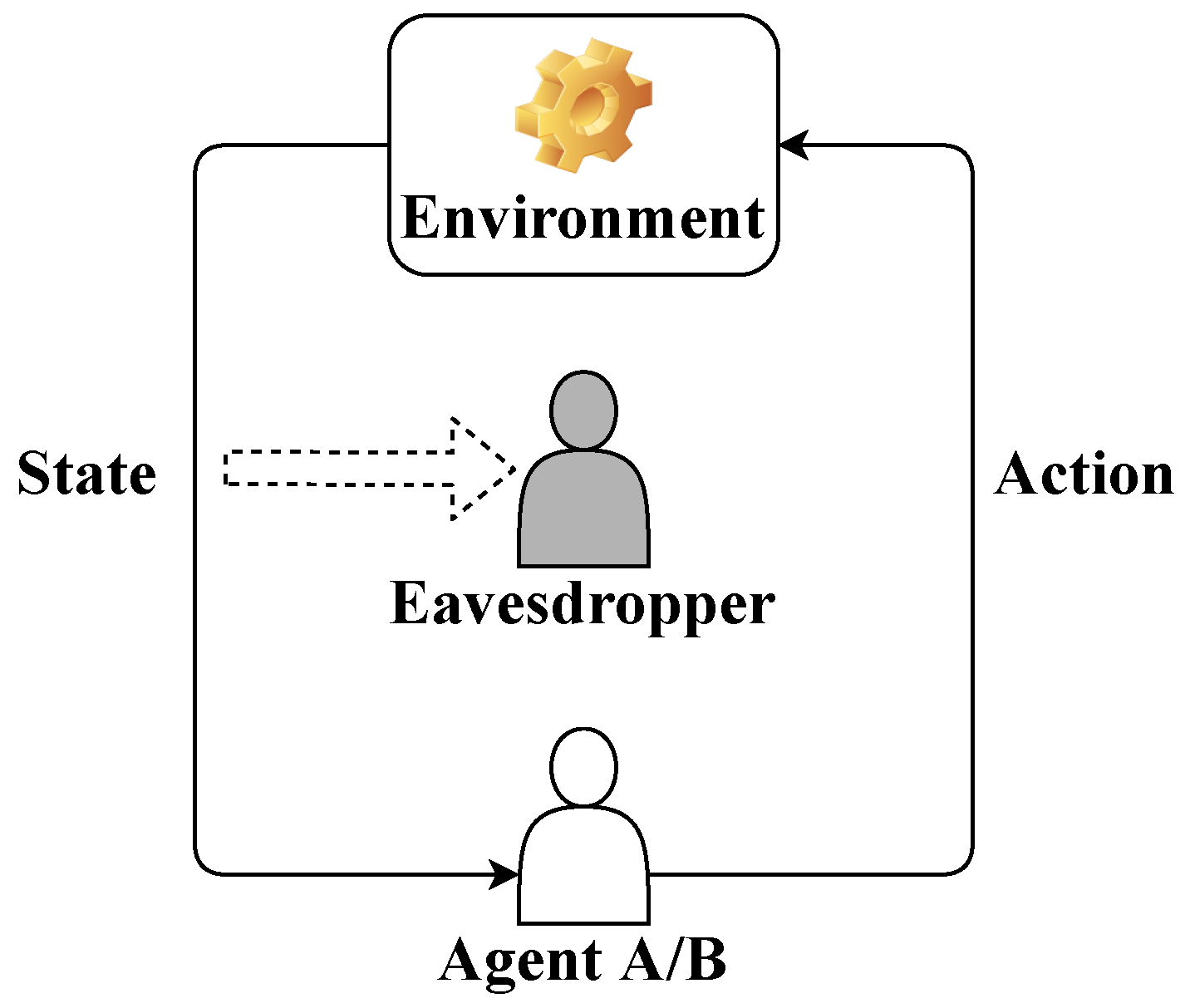
3. Agent Identity Privacy Problem in LQG Control

We consider an N-step LQG control in the presence of an eavesdropper as shown in Figure 1. There are two possible agents, Agent A and Agent B, which are with respect to a hypothesis $H=0$ and an alternative hypothesis $H=1$. We assume that the agents and the eavesdropper have perfect observations of the environment states. Based on the intercepted state sequence, the eavesdropper makes a binary hypothesis testing (A binary hypothesis is considered in this paper for simplification and can be extended to a multi-hypothesis.) to identify the current agent, which results in an agent identity privacy problem. To have a better understanding of the privacy problem, we give an example in the emerging application of autonomous vehicle. An autonomous vehicle can be controlled by a human driver (Agent A) or an autonomous driving system (Agent B). An adversary, who can be a compromised manager of the vehicle to everything (V2X) network, has access to the sensing data (environment state) of the autonomous vehicle and aims to attack the autonomous vehicle, e.g., to mislead the autonomous vehicle off the lane. To this end, the adversary needs to first identify if the current driver is the autonomous driving system by the intercepted sensing data sequence. The agent identity privacy problem commonly exists in intelligent autonomous systems, e.g., unmanned aerial vehicles and robots, where the autonomous control agents depending strongly on the sensing data are vulnerable to injection attacks and therefore the agent identities are privacy-sensitive.

The LQG control model for each agent is given as follows: For $H=0$ or $H=1$, $1\le i\le N$,

$$\begin{array}{c}{s}_{i+1}^{\left(H\right)}=\alpha s_i^{\left(H\right)}+\beta a_i^{\left(H\right)}+z_i,\end{array}$$

(1)

$$\begin{array}{c}{a}_i^{\left(H\right)}=F_i^{\left(H\right)}\left(s_i^{\left(H\right)}\right),\end{array}$$

(2)

$$\begin{array}{c}{r}_i^{\left(H\right)}=R^{\left(H\right)}\left(s_i^{\left(H\right)},a_i^{\left(H\right)}\right)=-{\theta }^{\left(H\right)}{\left(s_i^{\left(H\right)}\right)}^2-{\varphi }^{\left(H\right)}{\left(a_i^{\left(H\right)}\right)}^2,\end{array}$$

(3)

$$\begin{array}{c}{S}_1^{\left(H\right)}\sim b_1^{\left(H\right)}\triangleq \mathcal{N}({\mu }_1,{\sigma }_1^2),\end{array}$$

(4)

$$\begin{array}{c}{Z}_i\sim \mathcal{N}(0,{\omega }^2),\end{array}$$

(5)

where the parameters $\alpha \ne 0$, $\beta \ne 0$, ${\theta }^{\left(H\right)}>0$, ${\varphi }^{\left(H\right)}>0$, ${\mu }_1$, ${\sigma }_1^2>0$, and ${\omega }^2>0$ are given. The initial environment state $s_1^{\left(H\right)}$ is randomly generated following an independent Gaussian distribution. In the i-th time step, on observing the environment state $s_i^{\left(H\right)}$, the agent with respect to the hypothesis H employs the control policy $F_i^{\left(H\right)}$ to (randomly) determine an action $a_i^{\left(H\right)}$ as (2); the instantaneous control reward $r_i^{\left(H\right)}$ is jointly determined by the current state $s_i^{\left(H\right)}$ and action $a_i^{\left(H\right)}$ as (3); the next state $s_{i+1}^{\left(H\right)}$ is jointly determined by the current state $s_i^{\left(H\right)}$, the current action $a_i^{\left(H\right)}$, and $z_i$ randomly generated following an independent zero-mean Gaussian distribution as (1). In the standard LQG problem, the agent with respect to the hypothesis H only aims to maximize the expected accumulative reward by optimizing the control policies $F_{1:N}^{\left(H\right)}$:

$$\begin{array}{c}\hfill F_{1:N}^{\left(H\right)\ast }=arg\underset{F_{1:N}^{\left(H\right)}}{max}\mathbb{E}\left(\sum _{i=1}^N{R}^{\left(H\right)}\left(S_i^{\left(H\right)},A_i^{\left(H\right)}\right)\right).\end{array}$$

(6)

The optimal LQG control policy has been well established [35] and can be described as follows. For $H=0$ or $H=1$, $1\le i\le N$,

$$\begin{array}{c}{\tilde{\theta }}_{N+1}^{\left(H\right)}=0,\end{array}$$

(7)

$$\begin{array}{c}{\tilde{\theta }}_i^{\left(H\right)}=L^{\left(H\right)}\left({\tilde{\theta }}_{i+1}^{\left(H\right)}\right)={\theta }^{\left(H\right)}+{\tilde{\theta }}_{i+1}^{\left(H\right)}{\alpha }^2-\frac{{\left({\tilde{\theta }}_{i+1}^{\left(H\right)}\right)}^2{\alpha }^2{\beta }^2}{{\varphi }^{\left(H\right)}+{\tilde{\theta }}_{i+1}^{\left(H\right)}{\beta }^2}>0,\end{array}$$

(8)

$$\begin{array}{c}{\kappa }_i^{\left(H\right)\ast }=-\frac{{\tilde{\theta }}_{i+1}^{\left(H\right)}\alpha \beta }{{\varphi }^{\left(H\right)}+{\tilde{\theta }}_{i+1}^{\left(H\right)}{\beta }^2},\end{array}$$

(9)

$$\begin{array}{c}{F}_i^{\left(H\right)\ast }\left(s_i^{\left(H\right)}\right)={\kappa }_i^{\left(H\right)\ast }{s}_i^{\left(H\right)}.\end{array}$$

(10)

For $H=0$ or 1, it can be easily verified that the mapping $L^{\left(H\right)}$ is order-preserving, i.e., $L^{\left(H\right)}\left(x\right)\le L^H\left(x^{\prime }\right)$ if $0\le x\le x^{\prime }$. From the Kleene’s fixed point theorem [36], it follows that

$$\begin{array}{cc}\hfill {\tilde{\theta }}^{\left(H\right)}=& \underset{N\to \infty }{lim}\underset{N \mathrm{i}\mathrm{t}\mathrm{e}\mathrm{r}\mathrm{a}\mathrm{t}\mathrm{i}\mathrm{o}\mathrm{n}\mathrm{s}}{\underbrace{L^{\left(H\right)}(L^{\left(H\right)}(\cdots (L^{\left(H\right)}(L^{\left(H\right)}}}\left({\tilde{\theta }}_{N+1}^{\left(H\right)}\right)\left)\right)\cdots \left)\right)\hfill \\ \hfill =& {\theta }^{\left(H\right)}+{\tilde{\theta }}^{\left(H\right)}{\alpha }^2-\frac{{\left({\tilde{\theta }}^{\left(H\right)}\right)}^2{\alpha }^2{\beta }^2}{{\varphi }^{\left(H\right)}+{\tilde{\theta }}^{\left(H\right)}{\beta }^2}\hfill \\ \hfill =& \frac{\sqrt{{({\varphi }^{\left(H\right)}-{\theta }^{\left(H\right)}{\beta }^2-{\varphi }^{\left(H\right)}{\alpha }^2)}^2+4{\theta }^{\left(H\right)}{\varphi }^{\left(H\right)}{\beta }^2}-({\varphi }^{\left(H\right)}-{\theta }^{\left(H\right)}{\beta }^2-{\varphi }^{\left(H\right)}{\alpha }^2)}{2{\beta }^2}.\hfill \end{array}$$

(11)

Therefore, if we consider the asymptotic regime as $N\to \infty$, the optimal control polices are time-invariant: For $H=0$ or $H=1$, $i\ge 1$,

$$\begin{array}{c}{\kappa }^{\left(H\right)\ast }=-\frac{{\tilde{\theta }}^{\left(H\right)}\alpha \beta }{{\varphi }^{\left(H\right)}+{\tilde{\theta }}^{\left(H\right)}{\beta }^2},\end{array}$$

(12)

$$\begin{array}{c}{F}_i^{\left(H\right)\ast }\left(s_i^{\left(H\right)}\right)={\kappa }^{\left(H\right)\ast }{s}_i^{\left(H\right)}.\end{array}$$

(13)

For the agent identity privacy problem, we assume that the eavesdropper collects a sequence of environment states and carries out a binary hypothesis testing on the agent identity. Thus, the privacy risk can be measured by the hypothesis testing performance. In information theory, Kullback–Leibler divergence measures the “distance” between two probability distributions. When the value of the Kullback–Leibler divergence $\mathbb{D}\left(p_{S_{1:N}^{\left(1\right)}}||p_{S_{1:N}^{\left(0\right)}}\right)$ is smaller, the random environment state sequences $S_{1:N}^{\left(0\right)}$ and $S_{1:N}^{\left(1\right)}$ are statistically “closer” to each other and it is more difficult for the eavesdropper to identify the current agent, i.e., a poorer hypothesis testing performance and a lower privacy risk. In this paper, we employ the Kullback–Leibler divergence $\mathbb{D}\left(p_{S_{1:N}^{\left(1\right)}}||p_{S_{1:N}^{\left(0\right)}}\right)$ as the privacy risk measure.

Furthermore, we assume that both agents aim to improve their own expected accumulative rewards while only Agent B considers to reduce the privacy risk. This assumption makes sense in a lot of scenarios. In the aforementioned autonomous vehicle example, Agent A denotes the human driver and does not need to change the optimal driving style; Agent B denotes the autonomous driving system and can be reconfigured with respect to the human’s optimal driving style to improve the driving efficiency and to reduce the privacy risk. Under the assumption, Agent A takes the optimal LQG control policy as described by (7)–(10) with $H=0$. In the following, we focus on the privacy-preserving LQG control policy of Agent B. Taking into account the two design objectives of Agent B, we formulate the following optimization problem:

$$\begin{array}{c}\hfill F_{1:N}^{\left(1\right)★}=arg\underset{F_{1:N}^{\left(1\right)}}{max}\mathbb{E}\left(\sum _{i=1}^N{R}^{\left(1\right)}\left(S_i^{\left(1\right)},A_i^{\left(1\right)}\right)\right)-\lambda \mathbb{D}\left(p_{S_{1:N}^{\left(1\right)}}||p_{S_{1:N}^{\left(0\right)\ast }}\right),\end{array}$$

(14)

where $\lambda \ge 0$ denotes the privacy-preserving design weight; the random environment state sequence $S_{1:N}^{\left(0\right)\ast }$ is induced by the optimal LQG policy $F_{1:N}^{\left(0\right)\ast }$ of Agent A. It follows from the chain rule of Kullback–Leibler divergence and the Markovian property of the state sequences that the privacy risk measure can be further decomposed as

$$\begin{array}{cc}\hfill \mathbb{D}\left(p_{S_{1:N}^{\left(1\right)}}||p_{S_{1:N}^{\left(0\right)\ast }}\right)=& \mathbb{D}\left(p_{S_1^{\left(1\right)}}||p_{S_1^{\left(0\right)}}\right)+\sum _{i=2}^N\mathbb{D}\left(p_{S_i^{\left(1\right)}|S_{i-1}^{\left(1\right)}}||p_{S_i^{\left(0\right)\ast }|S_{i-1}^{\left(0\right)\ast }}\right)\hfill \\ \hfill =& \sum _{i=2}^N\mathbb{D}\left(p_{S_i^{\left(1\right)}|S_{i-1}^{\left(1\right)}}||p_{S_i^{\left(0\right)\ast }|S_{i-1}^{\left(0\right)\ast }}\right).\hfill \end{array}$$

(15)

It is obvious that the optimal privacy-preserving LQG control policy of Agent B depends on the value of $\lambda$. In the following two remarks, the optimal privacy-preserving LQG control policies are characterized for two special cases, $\lambda =0$ and $\lambda \to \infty$, respectively.

Remark 1.

When $\lambda =0$, Agent B only aims to maximize the expected accumulative reward $\mathbb{E}\left({\sum }_{i=1}^N{R}^{\left(1\right)}\left(S_i^{\left(1\right)},A_i^{\left(1\right)}\right)\right)$. In this case, the optimal privacy-preserving LQG policy of Agent B reduces to the optimal LQG policy of Agent B, i.e., $F_i^{\left(1\right)★}\left(s_i^{\left(1\right)}\right)=F_i^{\left(1\right)\ast }\left(s_i^{\left(1\right)}\right)={\kappa }_i^{\left(1\right)\ast }{s}_i^{\left(1\right)}$ for all $1\le i\le N$.

Remark 2.

When $\lambda \to \infty$, Agent B only aims to minimize the privacy risk, which is measured by the Kullback–Leibler divergence $\mathbb{D}\left(p_{S_{1:N}^{\left(1\right)}}||p_{S_{1:N}^{\left(0\right)\ast }}\right)$. In this case, the optimal privacy-preserving LQG policy of Agent B reduces to the optimal LQG policy of Agent A, i.e., $F_i^{\left(1\right)★}\left(s_i^{\left(1\right)}\right)=F_i^{\left(0\right)\ast }\left(s_i^{\left(1\right)}\right)={\kappa }_i^{\left(0\right)\ast }{s}_i^{\left(1\right)}$ for all $1\le i\le N$, and the minimum privacy risk is achieved, i.e., $\mathbb{D}\left(p_{S_{1:N}^{\left(1\right)★}}||p_{S_{1:N}^{\left(0\right)\ast }}\right)=0$.

When $0<\lambda <\infty$, we characterize the optimal privacy-preserving LQG control policies of Agent B in different forms in the following sections. For ease of reading, we list the parameters and their meanings in

Table 2. Parameters.

Parameter	Meaning	Parameter	Meaning
N	Number of steps	H	Agent identity binary hypothesis
$\alpha$, $\beta$	Time-invariant linear coefficients in the linear Gaussian dynamic model	$z_i$, ${\omega }^2$	Independent zero-mean Gaussian-distributed disturbance noise in the i-th step and its variance
$s_i^{\left(H\right)}$	State of the agent $\left(H\right)$ in the i-th step	$a_i^{\left(H\right)}$	Action of the agent $\left(H\right)$ in the i-th step
$F_i^{\left(H\right)}$	Policy of the agent $\left(H\right)$ in the i-th step	${\kappa }_i^{\left(H\right)}$	State feedback gain of a linear policy of the agent $\left(H\right)$ in the i-th step
$r_i^{\left(H\right)}$	Instantaneous control reward of the agent $\left(H\right)$ in the i-th step	$R^{\left(H\right)}$, ${\theta }^{\left(H\right)}$, ${\varphi }^{\left(H\right)}$	Time-invariant instantaneous quadratic control reward function of the agent $\left(H\right)$ and its coefficients
${\mu }_1$, ${\sigma }_1^2$	Mean and variance of the Gaussian-distributed initial state	$\lambda$	Privacy-preserving design weight

.

4. Deterministic Privacy-Preserving LQG Policy

When the privacy risk is not considered, as shown in (10), the optimal LQG control policy of Agent B is a deterministic linear mapping. In this section, we study the optimal deterministic privacy-preserving LQG policy of Agent B. Therefore, the policy of Agent B can be specified as: For $1\le i\le N$,

$$\begin{array}{c}\hfill F_i^{\left(1\right)}:\mathbb{R}\to \mathbb{R}.\end{array}$$

(16)

In the following theorem, we characterize the optimal deterministic privacy-preserving LQG policy of Agent B.

Theorem 1.

At each step, the optimal deterministic privacy-preserving LQG policy of Agent B with respect to the optimization problem (14) is a linear mapping as: For $1\le i\le N$,

$${\widehat{\theta }}_{N+1}^{\left(1\right)}=0,$$

(17)

$${\widehat{\theta }}_i^{\left(1\right)}=J_{N+1-i}\left({\widehat{\theta }}_{i+1}^{\left(1\right)}\right)={\theta }^{\left(1\right)}+{\widehat{\theta }}_{i+1}^{\left(1\right)}{\alpha }^2+\frac{\lambda }{2{\omega }^2}{\beta }^2{\left({\kappa }_i^{\left(0\right)\ast }\right)}^2-\frac{{\left(\frac{\lambda }{2{\omega }^2}{\beta }^2{\kappa }_i^{\left(0\right)\ast }-{\widehat{\theta }}_{i+1}^{\left(1\right)}\alpha \beta \right)}^2}{{\varphi }^{\left(1\right)}+{\widehat{\theta }}_{i+1}^{\left(1\right)}{\beta }^2+\frac{\lambda }{2{\omega }^2}{\beta }^2}>0,$$

(18)

$${\kappa }_i^{\left(1\right)★}=\frac{\frac{\lambda }{2{\omega }^2}{\beta }^2{\kappa }_i^{\left(0\right)\ast }-{\widehat{\theta }}_{i+1}^{\left(1\right)}\alpha \beta }{{\varphi }^{\left(1\right)}+{\widehat{\theta }}_{i+1}^{\left(1\right)}{\beta }^2+\frac{\lambda }{2{\omega }^2}{\beta }^2},$$

(19)

$$F_i^{\left(1\right)★}\left(s_i^{\left(1\right)}\right)={\kappa }_i^{\left(1\right)★}{s}_i^{\left(1\right)}.$$

(20)

Then, the maximum achievable weighted design objective of Agent B is

$$\begin{array}{c}\hfill \underset{F_{1:N}^{\left(1\right)}}{max}\mathbb{E}\left(\sum _{i=1}^N{R}^{\left(1\right)}\left(S_i^{\left(1\right)},A_i^{\left(1\right)}\right)\right)-\lambda \mathbb{D}\left(p_{S_{1:N}^{\left(1\right)}}||p_{S_{1:N}^{\left(0\right)\ast }}\right)=-{\widehat{\theta }}_1^{\left(1\right)}({\mu }_1^2+{\sigma }_1^2)-{\omega }^2\sum _{i=1}^{N-1}{\widehat{\theta }}_{i+1}^{\left(1\right)}.\end{array}$$

(21)

The proof of Theorem 1 is presented in Appendix A.

Remark 3.

When $\lambda =0$, it is easy to show that ${\kappa }_i^{\left(1\right)★}={\kappa }_i^{\left(1\right)\ast }$ for all $1\le i\le N$, i.e., the optimal deterministic privacy-preserving LQG policy is consistent with the optimal privacy-preserving LQG policy shown in Remark 1.

Remark 4.

It is easy to show that ${lim}_{\lambda \to \infty }{\kappa }_i^{\left(1\right)★}={\kappa }_i^{\left(0\right)\ast }$ for all $1\le i\le N$, i.e., the optimal deterministic privacy-preserving LQG policy is consistent with the optimal privacy-preserving LQG policy shown in Remark 2.

Remark 5.

Although the objective in (14) is a linear combination of the expected accumulative reward and the privacy risk measured by the Kullback–Leibler divergence, the optimal linear coefficient ${\kappa }_i^{\left(1\right)★}$ is a non-linear function of ${\kappa }_i^{\left(1\right)\ast }$ (the optimal linear coefficient with respect to only maximize the expected accumulative reward) and ${\kappa }_i^{\left(0\right)\ast }$ (the optimal linear coefficient with respect to only minimize the privacy risk) when we consider the deterministic privacy-preserving LQG control policy of Agent B.

Remark 6.

When Agent B employs the optimal deterministic privacy-preserving LQG policy at each step, the random state-action sequence is jointly Gaussian distributed.

In the asymptotic regime as $N\to \infty$, the optimal LQG control policy is time-invariant. In this case, the design of the optimal policy becomes an easier task. Theorem 2 gives a sufficient condition such that the optimal deterministic privacy-preserving LQG policy of Agent B is time-invariant in the asymptotic regime.

Theorem 2.

When the model parameters satisfy the following inequality

$$\begin{array}{c}\hfill \frac{\left|\frac{\lambda }{2{\omega }^2}{\beta }^4{\left({\kappa }^{\left(0\right)\ast }\right)}^2{\varphi }^{\left(1\right)}-\left({\varphi }^{\left(1\right)}{\alpha }^2+\frac{\lambda }{2{\omega }^2}{\beta }^2{\left(\alpha +\beta {\kappa }^{\left(0\right)\ast }\right)}^2\right)\left({\varphi }^{\left(1\right)}+\frac{\lambda }{2{\omega }^2}{\beta }^2\right)\right|}{{\left({\varphi }^{\left(1\right)}+\frac{\lambda }{2{\omega }^2}{\beta }^2\right)}^2}<1,\end{array}$$

(22)

the optimal deterministic privacy-preserving LQG policy of Agent B is time-invariant in the asymptotic regime. More specifically, $J_N(J_{N-1}(\cdots (J_2(J_1({\widehat{\theta }}_{N+1}^{(1)})))\cdots ))$ converges to the unique fixed point ${\widehat{\theta }}^{\left(1\right)}$ as

$$\begin{array}{cc}\hfill {\widehat{\theta }}^{(1)}=& \underset{N\to \infty }{lim}{J}_N(J_{N-1}(\cdots (J_2(J_1({\widehat{\theta }}_{N+1}^{(1)})))\cdots ))\hfill \\ \hfill =& {\theta }^{\left(1\right)}+{\alpha }^2{\widehat{\theta }}^{\left(1\right)}+\frac{\lambda }{2{\omega }^2}{\beta }^2{\left({\kappa }^{\left(0\right)\ast }\right)}^2-\frac{{\left(\frac{\lambda }{2{\omega }^2}{\beta }^2{\kappa }^{\left(0\right)\ast }-\alpha \beta {\widehat{\theta }}^{\left(1\right)}\right)}^2}{{\varphi }^{\left(1\right)}+{\beta }^2{\widehat{\theta }}^{\left(1\right)}+\frac{\lambda }{2{\omega }^2}{\beta }^2};\hfill \end{array}$$

(23)

and the time-invariant optimal deterministic privacy-preserving LQG policy of Agent B can be described by

$$\begin{array}{c}{\kappa }^{\left(1\right)★}=\frac{\frac{\lambda }{2{\omega }^2}{\beta }^2{\kappa }^{\left(0\right)\ast }-{\widehat{\theta }}^{\left(1\right)}\alpha \beta }{{\varphi }^{\left(1\right)}+{\widehat{\theta }}^{\left(1\right)}{\beta }^2+\frac{\lambda }{2{\omega }^2}{\beta }^2},\end{array}$$

(24)

$$\begin{array}{c}{F}_i^{\left(1\right)★}\left(s_i^{\left(1\right)}\right)={\kappa }^{\left(1\right)★}{s}_i^{\left(1\right)}.\end{array}$$

(25)

Under this condition, the asymptotic weighted design object rate of Agent B achieved by the time-invariant optimal deterministic privacy-preserving LQG policy is

$$\begin{array}{c}\hfill \underset{N\to \infty }{lim}\frac{1}{N}\underset{F_{1:N}^{\left(1\right)}}{max}\mathbb{E}\left(\sum _{i=1}^N{R}^{\left(1\right)}\left(S_i^{\left(1\right)},A_i^{\left(1\right)}\right)\right)-\lambda \mathbb{D}\left(p_{S_{1:N}^{\left(1\right)}}||p_{S_{1:N}^{\left(0\right)\ast }}\right)=-{\omega }^2{\widehat{\theta }}^{\left(1\right)}.\end{array}$$

(26)

The proof of Theorem 2 is given in Appendix B.

5. Random Privacy-Preserving LQG Policy

As shown in Theorem 1, the optimal deterministic privacy-preserving LQG policy of Agent B is a linear mapping. In this section, we first discuss the optimal random privacy-preserving LQG policy and then consider a particular random policy by extending the deterministic linear mapping to the linear Gaussian random policy for Agent B. Here, the random policy of Agent B can be specified as: For $1\le i\le N$,

$$\begin{array}{c}\hfill F_i^{\left(1\right)}:\mathbb{R}\times \mathbb{R}\to {\mathbb{R}}_{\ge 0}.\end{array}$$

(27)

With slight abuse of notation, we denote the condition probability (density) of taking the action $a_i^{\left(1\right)}\in \mathbb{R}$ given the state $s_i^{\left(1\right)}\in \mathbb{R}$ and the random policy $F_i^{\left(1\right)}$ by $F_i^{\left(1\right)}\left(a_i^{\left(1\right)}\left|s_i^{\left(1\right)}\right.\right)\in {\mathbb{R}}_{\ge 0}$.

It can be easily shown that the optimal random privacy-preserving LQG policy of Agent B in the final step $F_N^{\left(1\right)★}$ reduces to the deterministic linear mapping in (A2). For $1\le i\le N-1$, it follows from the backward dynamic programming that the optimal random privacy-preserving LQG policy of Agent B in the i-th step does not reduce to a deterministic linear mapping in general. That is because the conditional probability distribution $p_{S_{i+1}^{\left(1\right)}|S_i^{\left(1\right)}}$ given a random policy $F_i^{\left(1\right)}$ is a Gaussian mixture model and then the Kullback–Leibler divergence $\mathbb{D}\left(p_{S_{i+1}^{\left(1\right)}|S_i^{\left(1\right)}}||p_{S_{i+1}^{\left(0\right)\ast }|S_i^{\left(0\right)\ast }}\right)$ between a Gaussian mixture model and a Gaussian distribution generally does not reduce to the quadratic mean of $A_i^{\left(1\right)}-{\kappa }_i^{\left(0\right)\ast }{S}_i^{\left(1\right)}$ as (A5). To the best of our knowledge, there is no analytically tractable formula for Kullback–Leibler divergence between Gaussian mixture models and only approximations are available [37,38,39]. Therefore, we do not give the close-form solution of the optimal random privacy-preserving LQG policy in this paper.

In what follows, we focus on the linear Gaussian random policy: For $1\le i\le N$,

$$\begin{array}{c}\hfill F_i^{\left(1\right)}\left(s_i^{\left(1\right)}\right)={\kappa }_i^{\left(1\right)}{s}_i^{\left(1\right)}+w_i^{\left(1\right)},\end{array}$$

(28)

where $w_i^{\left(1\right)}$ is the realization of an independent zero-mean Gaussian random process noise $W_i^{\left(1\right)}\sim \mathcal{N}(0,{\delta }_i^2)$. Thus, a linear Gaussian random policy $F_i^{\left(1\right)}$ can be completely described by the parameters $\left({\kappa }_i^{\left(1\right)},{\delta }_i^2\right)$. Theorem 3 characterizes the optimal linear Gaussian random privacy-preserving LQG policy of Agent B.

Theorem 3.

At each step, the optimal linear Gaussian random privacy-preserving LQG policy of Agent B with respect to the optimization problem (14) is the same deterministic linear mapping as in Theorem 1.

The proof of Theorem 3 is presented in Appendix C.

Remark 7.

Adding an independent zero-mean Gaussian random process noise to the linear mapping of the optimal deterministic privacy-preserving LQG policy cannot improve the performance of Agent B.

6. Numerical Experiments

6.1. Convergence of the Sequence $\left({\widehat{\theta }}_{N+1}^{\left(1\right)},{\widehat{\theta }}_N^{\left(1\right)},{\widehat{\theta }}_{N-1}^{\left(1\right)},\cdots \right)$

When the constraint (22) in Theorem 2 is satisfied, we first illustrate the convergence of the sequence $\left({\widehat{\theta }}_{N+1}^{\left(1\right)},{\widehat{\theta }}_N^{\left(1\right)},{\widehat{\theta }}_{N-1}^{\left(1\right)},\cdots \right)$. In addition to the default model parameters in

Table 3. Default model parameters.

Parameter	${\mathit{\mu }}_1$	${\mathit{\sigma }}_1^2$	$\mathit{\alpha }$	$\mathit{\beta }$	${\mathit{\omega }}^2$	${\mathit{\theta }}^{\left(0\right)}$	${\mathit{\varphi }}^{\left(0\right)}$
Value	1	1	1	$0.5$	$0.5$	1	16

, we set ${\theta }^{\left(1\right)}=8$, ${\varphi }^{\left(1\right)}=1$, and let the privacy-preserving design weight $\lambda =1$, 5 or 10. By using these parameters, it can be easily verified that the constraint (22) is satisfied. Figure 2 shows that ${\widehat{\theta }}_{N+1-k}^{(1)}=J_k(J_{k-1}(\cdots (J_2(J_1({\widehat{\theta }}_{N+1}^{(1)})))\cdots ))$ converges after $k=20$ iterations for different values of $\lambda$. Furthermore, different convergence patterns can be observed for different values of $\lambda$.

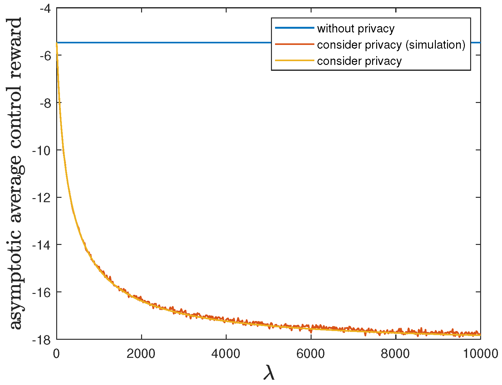
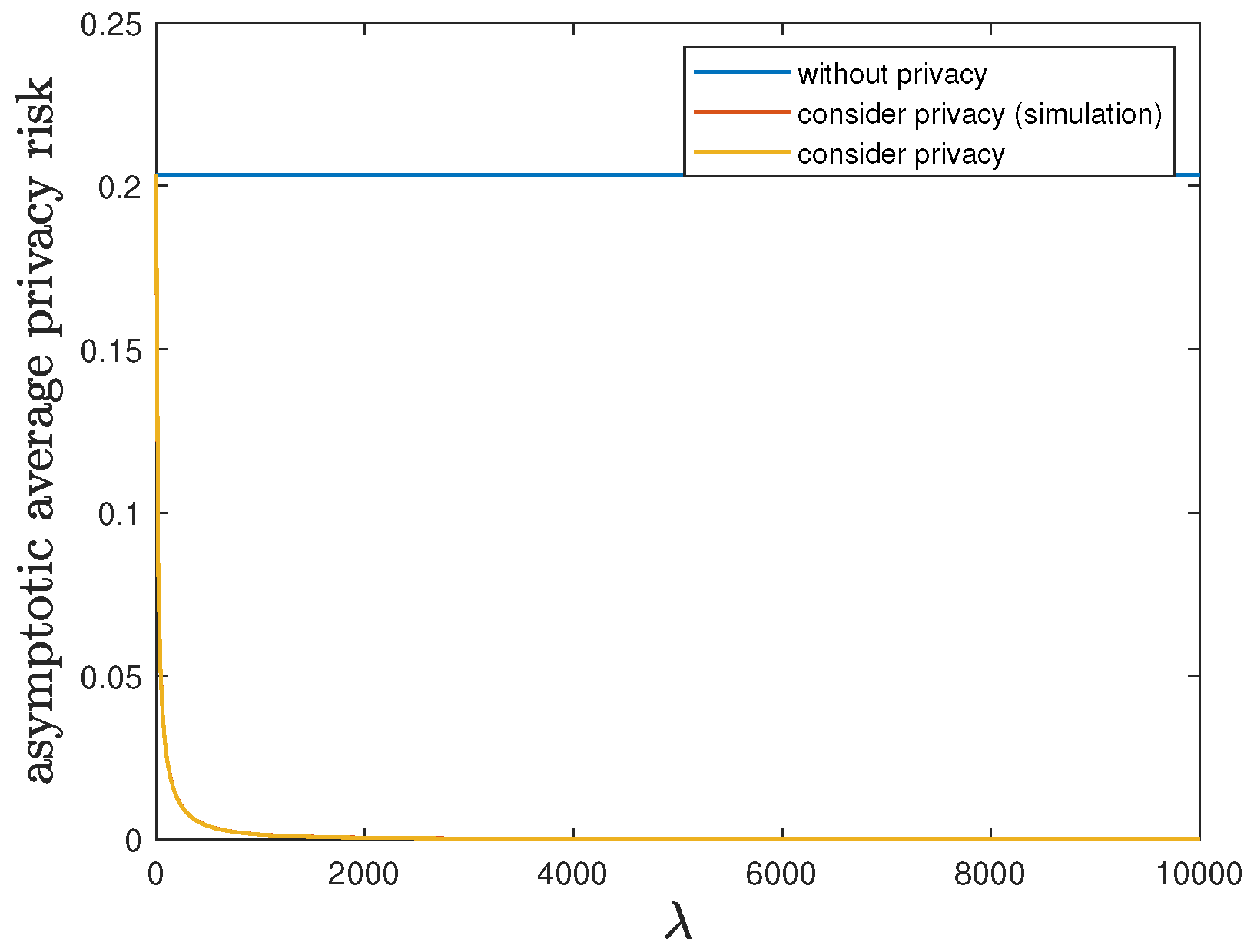
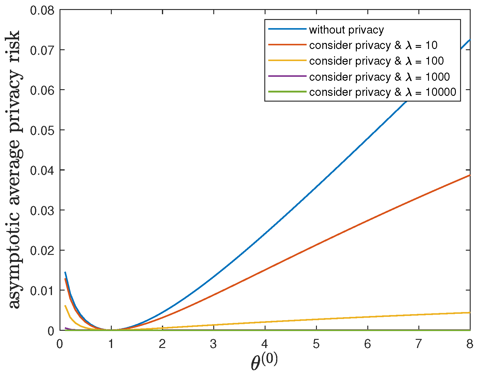
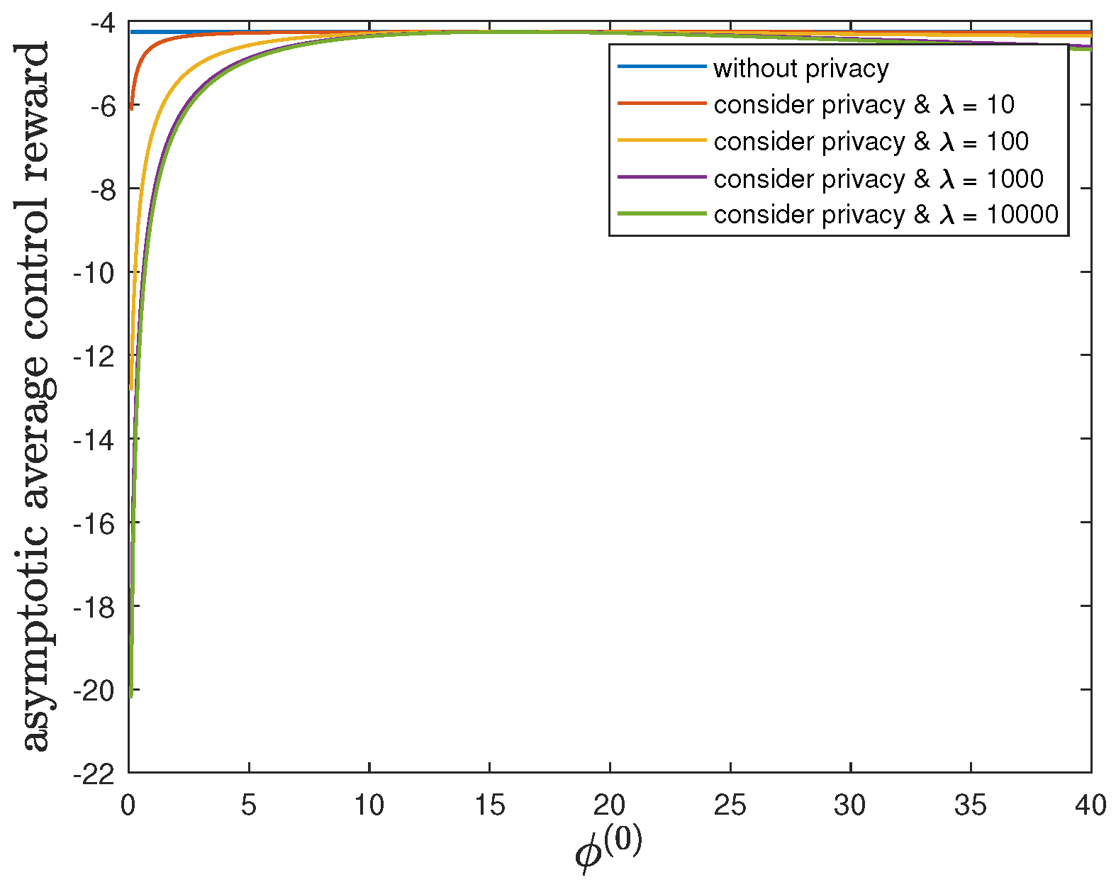
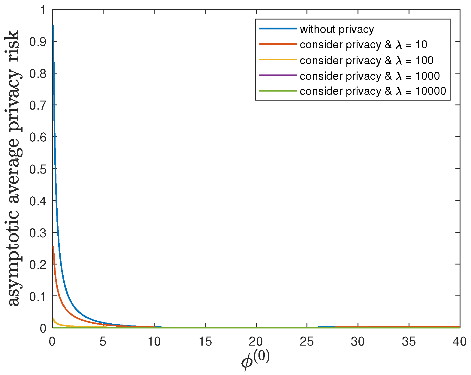
6.2. Impact of the Privacy-Preserving Design Weight $\lambda$

Here, we show the impact of the privacy-preserving design weight $\lambda$ on the trade-off between the control reward of Agent B and the privacy risk. We use the same parameters as in Section 6.1, but allow $0\le \lambda \le$ 10,000. Then, Theorem 2 is applicable and therefore the optimal deterministic privacy-preserving LQG policy of Agent B is time-invariant in the asymptotic regime. Figure 3 and Figure 4 show that both the asymptotic average control reward ${lim}_{N\to \infty }\frac{1}{N}\mathbb{E}\left({\sum }_{i=1}^N{R}^{(1)}\left(S_i^{(1)★},A_i^{(1)★}\right)\right)$ and the asymptotic average privacy risk ${lim}_{N\to \infty }\frac{1}{N}\mathbb{D}\left(p_{S_{1:N}^{\left(1\right)★}}||p_{S_{1:N}^{\left(0\right)\ast }}\right)$ achieved by the time-invariant optimal deterministic privacy-preserving LQG policy of Agent B decrease as $\lambda$ increases, i.e., the control reward of Agent B is degraded while the privacy is enhanced. When the privacy risk is not considered, the best control reward of Agent B is achieved at the cost of the highest privacy risk.

In addition to the analytical results, we also present the simulation results by considering privacy in Figure 3 and Figure 4. Given $0\le \lambda \le$ 10,000, we employ the corresponding time-invariant optimal deterministic privacy-preserving LQG policy of Agent B and run the 10,000-step privacy-preserving LQG control with 100 randomly generated initial states. Then, the average control reward and the average privacy risk are evaluated and compared with the analytical results of asymptotic average control reward and asymptotic average privacy risk, respectively. As shown in Figure 3 and Figure 4, the simulation results match quite well with the analytical results, which validates our analytical results.

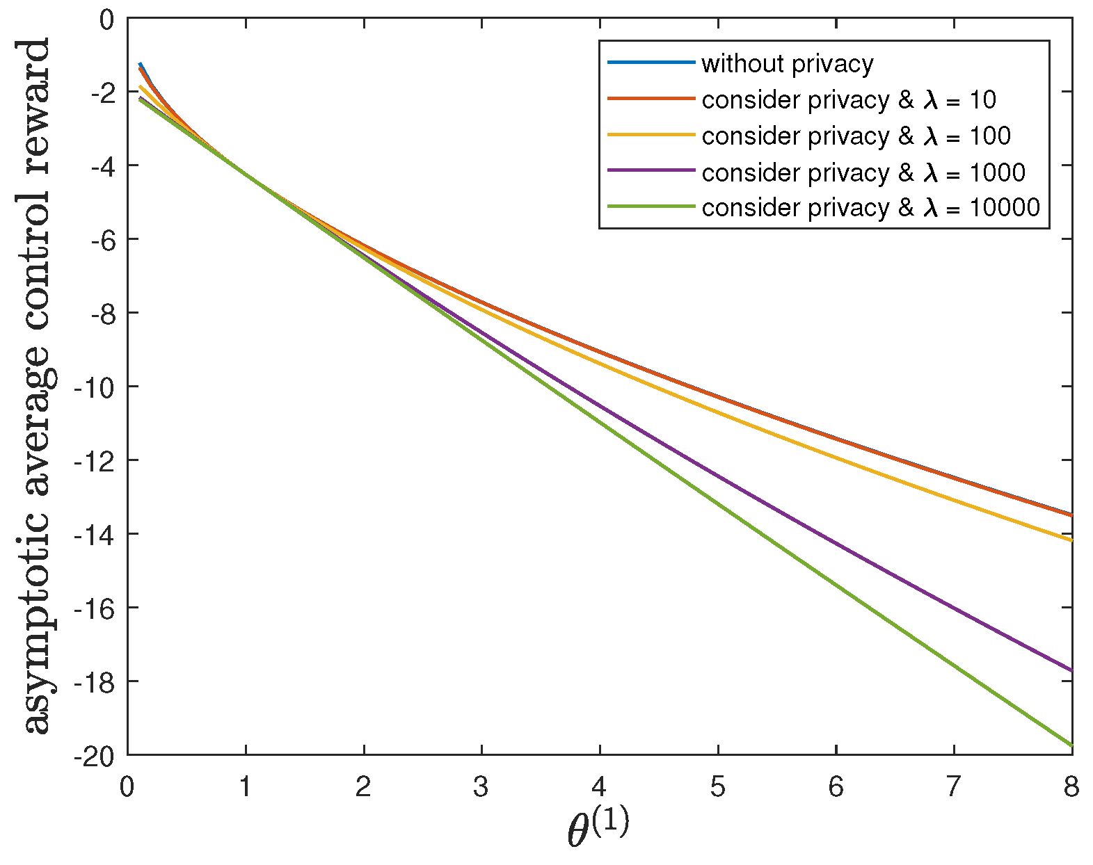
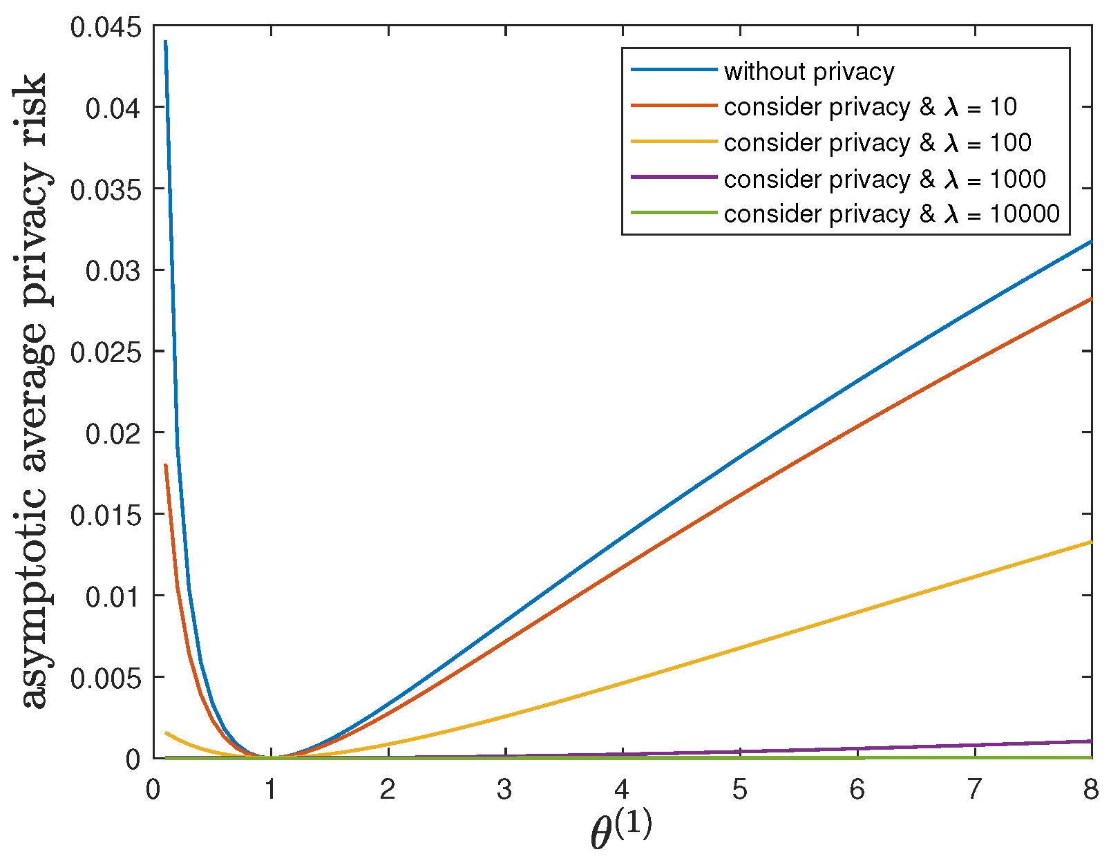
6.3. Impact of Parameter ${\theta }^{\left(1\right)}$

Here, we study the impact of the parameter ${\theta }^{\left(1\right)}$ on the control reward of Agent B and the privacy risk. In addition to the default model parameters in Table 3, we set ${\varphi }^{\left(1\right)}={\varphi }^{\left(0\right)}=16$ and allow $0.01\le {\theta }^{\left(1\right)}\le 8$, $\lambda =0$ (without privacy), 10, 100, 1000 or 10,000. It can be verified that Theorem 2 holds for those model parameters. For all $0.01\le {\theta }^{\left(1\right)}\le 8$ and by increasing the value of $\lambda$, Figure 5 and Figure 6 show a trade-off between the control reward of Agent B and the privacy risk, which is consistent with the previous observations. For $\lambda =0$, 10, 100, 1000 or 10,000, Figure 5 shows that the asymptotic average control reward of Agent B decreases as ${\theta }^{\left(1\right)}$ increases. This is reasonable since $-{\theta }^{\left(1\right)}$ is the quadratic coefficient in the instantaneous reward function $R^{\left(1\right)}$. For $\lambda =0$, 10, 100, 1000 or 10,000, Figure 6 shows that the asymptotic average privacy risk has a pattern to decrease first, then to increase, and to achieve the minimum value 0 when ${\theta }^{\left(1\right)}={\theta }^{\left(0\right)}=1$. When ${\theta }^{\left(1\right)}={\theta }^{\left(0\right)}=1$, both agents have the same instantaneous reward function and employ the same optimal LQG control policy, which leads to the same state sequence distribution under both hypotheses and the minimum value 0 of the Kullback–Leibler divergence. As ${\theta }^{\left(1\right)}$ deviates from the value of ${\theta }^{\left(0\right)}$, the agents have more different instantaneous reward functions, which lead to more different state sequence distributions under both hypotheses and a larger value of the Kullback–Leibler divergence.

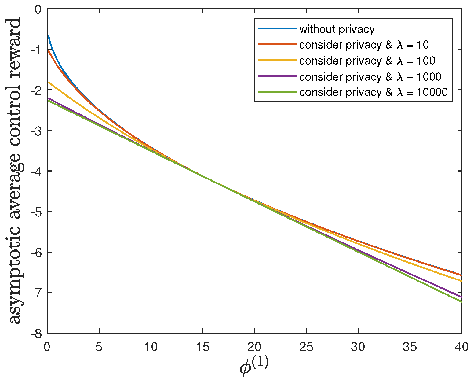
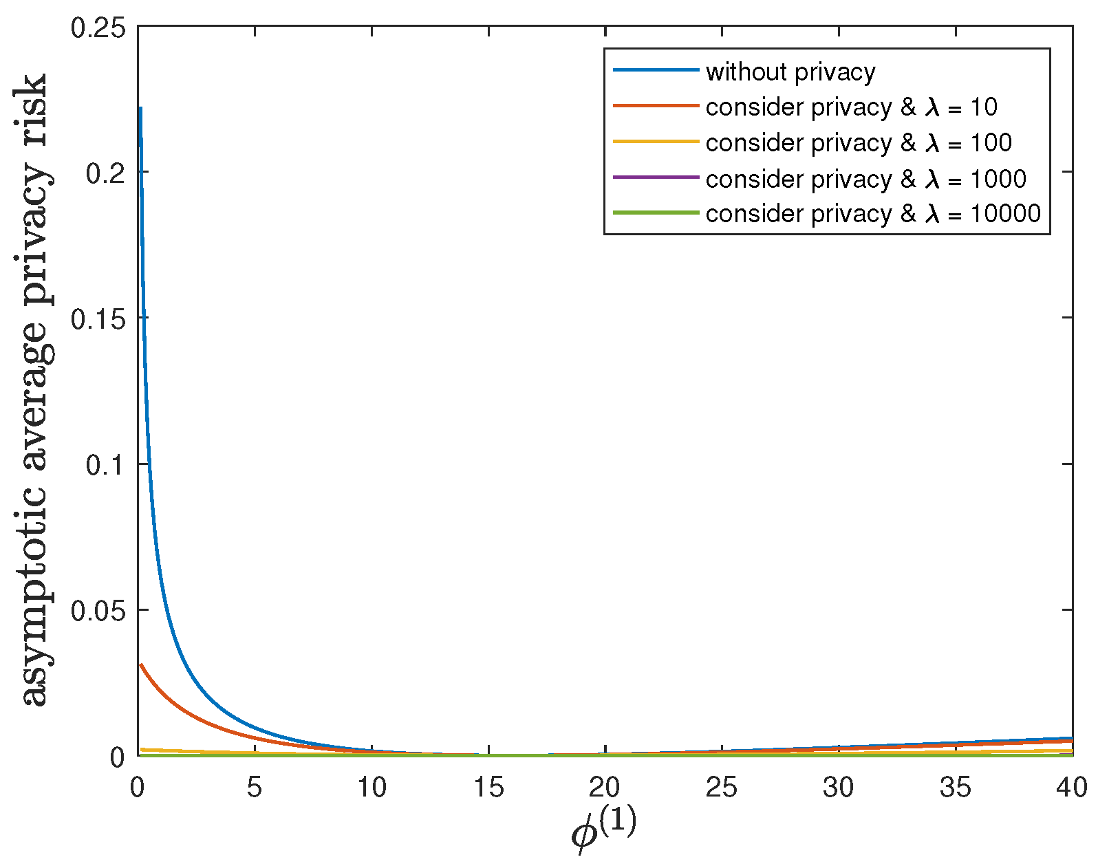
6.4. Impact of Parameter ${\varphi }^{\left(1\right)}$

Here, we show the impact of the parameter ${\varphi }^{\left(1\right)}$ on the control reward of Agent B and the privacy risk. In addition to the default model parameters in Table 3, we set ${\theta }^{\left(1\right)}={\theta }^{\left(0\right)}=1$ and allow $0.01\le {\varphi }^{\left(1\right)}\le 40$, $\lambda =0$ (without privacy), 10, 100, 1000 or 10,000. It can be verified that Theorem 2 holds for those model parameters. For all $0.01\le {\varphi }^{\left(1\right)}\le 40$ and by increasing the value of $\lambda$, Figure 7 and Figure 8 also show a trade-off between the control reward of Agent B and the privacy risk. For $\lambda =0$, 10, 100, 1000 or 10,000, Figure 7 shows that the asymptotic average control reward of Agent B decreases as ${\varphi }^{\left(1\right)}$ increases. This is because $-{\varphi }^{\left(1\right)}$ is the other quadratic coefficient in the instantaneous reward function $R^{\left(1\right)}$. For $\lambda =0$, 10, 100, 1000 or 10,000, Figure 8 shows that the asymptotic average privacy risk has a similar pattern to decrease first, then to increase, and to achieve the minimum value 0 when ${\varphi }^{\left(1\right)}={\varphi }^{\left(0\right)}=16$. This pattern can be similarly explained as Section 6.3.

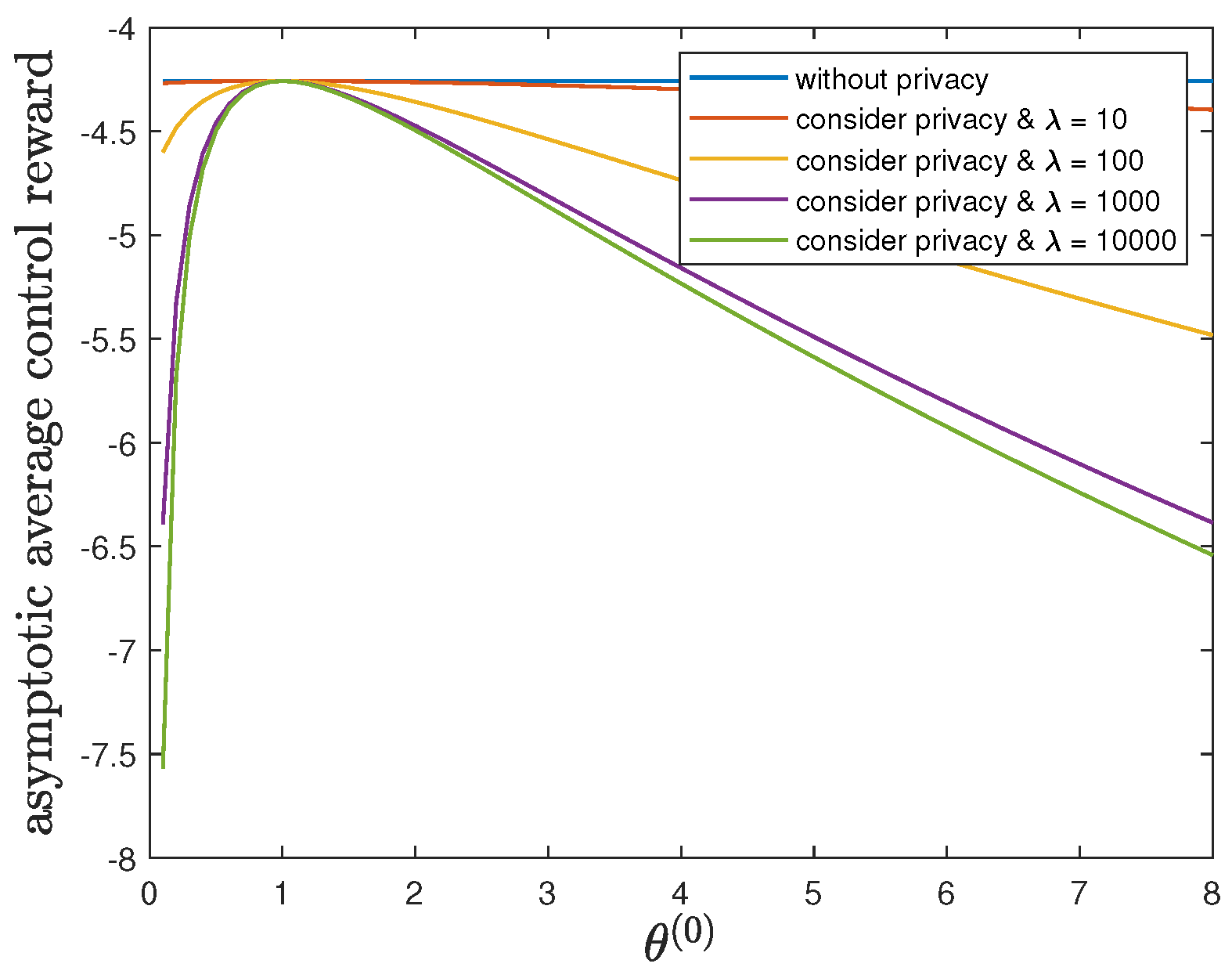
6.5. Impact of Parameter ${\theta }^{\left(0\right)}$

By fixing ${\theta }^{\left(1\right)}=1$ and ${\varphi }^{\left(1\right)}={\varphi }^{\left(0\right)}=16$, we study the impact of the parameter ${\theta }^{\left(0\right)}$ on the control reward of Agent B and the privacy risk. In addition to the default model parameters in Table 3, we allow $0.01\le {\theta }^{\left(0\right)}\le 8$ and $\lambda =0$ (without privacy), 10, 100, 1000 or 10,000. It can be verified that Theorem 2 holds for those model parameters. For all $0.01\le {\theta }^{\left(0\right)}\le 8$ and by increasing the value of $\lambda$, Figure 9 and Figure 10 show a trade-off between the control reward of Agent B and the privacy risk. For $\lambda =0$, 10, 100, 1000 or 10,000, Figure 9 and Figure 10 show that the asymptotic average control reward of Agent B achieves the maximum value while the asymptotic average privacy risk achieves the minimum value 0 when ${\theta }^{\left(1\right)}={\theta }^{\left(0\right)}=1$. In this case, both agents have the same instantaneous reward function and employ the same optimal LQG control policy, which maximizes their control rewards, leads to the same state sequence distribution under both hypotheses, and therefore achieves the minimum value 0 of the Kullback–Leibler divergence.

6.6. Impact of Parameter ${\varphi }^{\left(0\right)}$

By fixing ${\varphi }^{\left(1\right)}=16$ and ${\theta }^{\left(1\right)}={\theta }^{\left(0\right)}=1$, we study the impact of the parameter ${\varphi }^{\left(0\right)}$ on the control reward of Agent B and the privacy risk. In addition to the default model parameters in Table 3, we allow $0.01\le {\varphi }^{\left(0\right)}\le 40$ and $\lambda =0$ (without privacy), 10, 100, 1000 or 10,000. From Figure 11 and Figure 12, we have similar observations of the impact of ${\varphi }^{\left(0\right)}$ as in Section 6.5. These observations here can be similarly explained as well.

7. Conclusions

In this paper, we consider the agent identity privacy problem in the scalar LQG control. Regarding this novel privacy problem, we model it as an adversarial binary hypothesis testing and employ the Kullback–Leibler divergence to measure the privacy risk. We then formulate a novel privacy-preserving LQG control optimization by taking into account both the accumulative control reward of Agent B and the privacy risk. We prove that the optimal deterministic privacy-preserving LQG control policy of Agent B is a linear mapping, which is consistent with the standard LQG. We further show that the random policy formulated by adding an independent Gaussian random process noise to the optimal deterministic privacy-preserving LQG policy cannot improve the performance. We also give a sufficient condition to guarantee the time-invariant optimal deterministic privacy-preserving LQG policy in the asymptotic regime.

This research can be extended in our future works. Studying the general random policy of Agent B is an interesting extension. This theoretic study can be extended to develop privacy-preserving reinforcement learning algorithms. The problem can also be extended and formulated as a non-cooperative game of multiple agents with conflicting objectives, where some agents only aim to optimize their own accumulative control rewards while the other agents consider the agent identity privacy risk in addition to their own accumulative control rewards.

References

1. Mnih, V.; Kavukcuoglu, K.; Silver, D.; Rusu, A.A.; Veness, J.; Bellemare, M.G.; Graves, A.; Riedmiller, M.; Fidjel, A.K.; Ostrovski, G.; et al. Human-level control through deep reinforcement learning. Nature 2015, 518, 529–533. [Google Scholar] [CrossRef] [PubMed]
2. Huang, S.; Papernot, N.; Goodfellow, I.; Duan, Y.; Abbeel, P. Adversarial attacks on neural network policies. arXiv 2016, arXiv:1702.02284. [Google Scholar]
3. Lin, Y.C.; Hong, Z.W.; Liao, Y.H.; Shih, M.L.; Liu, M.Y.; Min, S. Tactics of adversarial attack on deep reinforcement learning agents. In Proceedings of the 2017 International Joint Conference on Artificial Intelligence, Melbourne, Australia, 19–25 August 2017; pp. 3756–3762. [Google Scholar]
4. Behzadan, V.; Munir, A. Vulnerability of deep reinforcement learning to policy induction attacks. In Proceedings of the MLDM 2017, New York, NY, USA, 15–20 July 2017; pp. 262–275. [Google Scholar]
5. Russo, A.; Proutiere, A. Optimal attacks on reinforcement learning policies. arXiv 2019, arXiv:1907.13548. [Google Scholar]
6. Goodfellow, I.; Shlens, J.; Szegedy, C. Explaining and harnessing adversarial examples. In Proceedings of the ICLR 2015, San Diego, CA, USA, 7–9 May 2015. [Google Scholar]
7. Tramer, F.; Kurakin, A.; Papernot, N.; Goodfellow, I.; Boneh, D.; McDaniel, P. Ensemble adversarial training: Attacks and defenses. In Proceedings of the ICLR 2018, Vancouver, BC, Canada, 30 April–3 May 2018. [Google Scholar]
8. Sinha, A.; Namkoong, H.; Duchi, J. Certifying some distributional robustness with principled adversarial training. In Proceedings of the ICLR 2018, Vancouver, BC, Canada, 30 April–3 May 2018. [Google Scholar]
9. Zheng, S.; Song, Y.; Leung, T.; Goodfellow, I. Improving the robustness of deep neural networks via stability training. In Proceedings of the CVPR 2016, Las Vegas, NV, USA, 27–30 June 2016. [Google Scholar]
10. Yan, Z.; Guo, Y.; Zhang, C. Deep defense: Training DNNs with improved adversarial robustness. In Proceedings of the NIPS 2018, Montréal, QC, Canada, 3–8 December 2018. [Google Scholar]
11. Shapley, L. Stochastic games. Proc. Natl. Acad. Sci. USA 1953, 39, 1095–1100. [Google Scholar] [CrossRef] [PubMed] [Green Version]
12. Gleave, A.; Dennis, M.; Wild, C.; Kant, N.; Levine, S.; Russell, S. Adversarial policies: Attacking deep reinforcement learning. In Proceedings of the ICLR 2020, Addis Ababa, Ethiopia, 26–30 April 2020. [Google Scholar]
13. Pinto, L.; Davidson, J.; Sukthankar, R.; Gupta, A. Robust adversarial reinforcement learning. In Proceedings of the ICML 2017, Sydney, NSW, Australia, 6–11 August 2017; pp. 2817–2826. [Google Scholar]
14. Horak, K.; Zhu, Q.; Bosansky, B. Manipulating adversary’s belief: A dynamic game approach to deception by design for proactive network security. In Proceedings of the GameSec 2017, Vienna, Austria, 23–25 October 2017; pp. 273–294. [Google Scholar]
15. Crawford, V.P.; Sobel, J. Strategic information transmission. Econometrica 1982, 50, 1431–1451. [Google Scholar] [CrossRef]
16. Saritas, S.; Yuksel, S.; Gezici, S. Nash and Stackelberg equilibria for dynamic cheap talk and signaling games. In Proceedings of the ACC 2017, Seattle, WA, USA, 24–26 May 2017; pp. 3644–3649. [Google Scholar]
17. Saritas, S.; Shereen, E.; Sandberg, H.; Dán, G. Adversarial attacks on continuous authentication security: A dynamic game approach. In Proceedings of the GameSec 2019, Stockholm, Sweden, 30 October–1 November 2019; pp. 439–458. [Google Scholar]
18. Li, Z.; Dán, G. Dynamic cheap talk for robust adversarial learning. In Proceedings of the GameSec 2019, Stockholm, Sweden, 30 October–1 November 2019; pp. 297–309. [Google Scholar]
19. Li, Z.; Dán, G.; Liu, D. A game theoretic analysis of LQG control under adversarial attack. In Proceedings of the IEEE CDC 2020, Jeju Island, Korea, 14–18 December 2020; pp. 1632–1639. [Google Scholar]
20. Osogami, T. Robust partially observable Markov decision process. In Proceedings of the ICML 2015, Lille, France, 6–11 July 2015. [Google Scholar]
21. Sayin, M.O.; Basar, T. Secure sensor design for cyber-physical systems against advanced persistent threats. In Proceedings of the GameSec 2017, Vienna, Austria, 23–25 October 2017; pp. 91–111. [Google Scholar]
22. Sayin, M.O.; Akyol, E.; Basar, T. Hierarchical multistage Gaussian signaling games in noncooperative communication and control systems. Automatica 2019, 107, 9–20. [Google Scholar] [CrossRef] [Green Version]
23. Sun, C.; Li, Z.; Wang, C. Adversarial linear quadratic regulator under falsified actions. In Proceedings of the ICASSP 2022—2022 IEEE International Conference on Acoustics, Speech and Signal Processing (ICASSP), Singapore, 23–27 May 2022. [Google Scholar]
24. Zhang, R.; Venkitasubramaniam, P. Stealthy control signal attacks in linear quadratic Gaussian control systems: Detectability reward tradeoff. IEEE Trans. Inf. Forensics Secur. 2017, 12, 1555–1570. [Google Scholar] [CrossRef]
25. Ren, X.X.; Yang, G.H. Kullback-Leibler divergence-based optimal stealthy sensor attack against networked linear quadratic Gaussian systems. IEEE Trans. Cybern. 2021, 1–10. [Google Scholar] [CrossRef] [PubMed]
26. Venkitasubramaniam, P. Privacy in stochastic control: A Markov decision process perspective. In Proceedings of the Allerton 2013, Monticello, IL, USA, 2–4 October 2013; pp. 381–388. [Google Scholar]
27. Ny, J.L.; Pappas, G.J. Differentially private filtering. IEEE Trans. Autom. Control. 2013, 59, 341–354. [Google Scholar]
28. Hale, M.T.; Egerstedt, M. Cloud-enabled differentially private multiagent optimization with constraints. IEEE Trans. Control. Netw. Syst. 2017, 5, 1693–1706. [Google Scholar] [CrossRef] [Green Version]
29. Hale, M.; Jones, A.; Leahy, K. Privacy in feedback: The differentially private LQG. In Proceedings of the ACC 2018, Milwaukee, WI, USA, 27–29 June 2018; pp. 3386–3391. [Google Scholar]
30. Hawkins, C.; Hale, M. Differentially private formation control. In Proceedings of the IEEE CDC 2020, Jeju Island, Korea, 14–18 December 2020; pp. 6260–6265. [Google Scholar]
31. Dwork, C. Differential privacy. In Proceedings of the ICALP 2006, Venice, Italy, 10–14 July 2006; pp. 1–12. [Google Scholar]
32. Wang, B.; Hegde, N. Privacy-preserving Q-learning with functional noise in continuous spaces. In Proceedings of the NeurIPS 2019, Vancouver, BC, Canada, 8–14 December 2019. [Google Scholar]
33. Alexandru, A.B.; Pappas, G.J. Encrypted LQG using labeled homomorphic encryption. In Proceedings of the ACM/IEEE ICCPS 2019, Montreal, QC, Canada, 16–18 April 2019. [Google Scholar]
34. Arora, S.; Doshi, P. A survey of inverse reinforcement learning: Challenges, methods and progress. Artif. Intell. 2021, 297, 103500. [Google Scholar] [CrossRef]
35. Soderstrom, T. Discrete-Time Stochastic Systems; Springer: Berlin/Heidelberg, Germany, 2002. [Google Scholar]
36. Baranga, A. The contraction principle as a particular case of Kleene’s fixed point theorem. Discret. Math. 1991, 98, 75–79. [Google Scholar] [CrossRef] [Green Version]
37. Hershey, J.R.; Olsen, P.A. Approximating the Kullback Leibler divergence between Gaussian mixture models. In Proceedings of the IEEE ICASSP 2007, Honolulu, HI, USA, 15–20 April 2007. [Google Scholar]
38. Durrieu, J.; Thiran, J.; Kelly, F. Lower and upper bounds for approximation of the Kullback-Leibler divergence between Gaussian mixture models. In Proceedings of the IEEE ICASSP 2012, Kyoto, Japan, 25–30 March 2012. [Google Scholar]
39. Cui, S.; Datcu, M. Comparison of Kullback-Leibler divergence approximation methods between Gaussian mixture models for satellite image retrieval. In Proceedings of the IEEE IGARSS 2015, Milan, Italy, 26–31 July 2015. [Google Scholar]
Figure 1. LQG control in the presence of an eavesdropper.
Entropy 24 00856 g001
Figure 2. For λ = 1 , 5 or 10, the convergence of θ ^ N + 1 k ( 1 ) = J k ( J k 1 ( ( J 2 ( J 1 ( θ ^ N + 1 ( 1 ) ) ) ) ) ) .
Entropy 24 00856 g002
Figure 3. When 0 λ 10,000, comparison of the asymptotic average control reward lim N 1 N E i = 1 N R ( 1 ) S i ( 1 ) , A i ( 1 ) achieved by the time-invariant optimal LQG policy of Agent B and the asymptotic average control reward lim N 1 N E i = 1 N R ( 1 ) S i ( 1 ) , A i ( 1 ) achieved by the time-invariant optimal deterministic privacy-preserving LQG policy of Agent B.
Entropy 24 00856 g003
Figure 4. When 0 λ 10,000, comparison of the asymptotic average privacy risk lim N 1 N D p S 1 : N ( 1 ) | | p S 1 : N ( 0 ) achieved by the time-invariant optimal LQG policy of Agent B and the asymptotic average privacy risk lim N 1 N D p S 1 : N ( 1 ) | | p S 1 : N ( 0 ) achieved by the time-invariant optimal deterministic privacy-preserving LQG policy of Agent B.
Entropy 24 00856 g004
Figure 5. For 0.01 θ ( 1 ) 8 and λ = 0 (without privacy), 10, 100, 1000 or 10,000, comparison of the asymptotic average control reward lim N 1 N E i = 1 N R ( 1 ) S i ( 1 ) , A i ( 1 ) achieved by the time-invariant optimal LQG policy of Agent B and the asymptotic average control reward lim N 1 N E i = 1 N R ( 1 ) S i ( 1 ) , A i ( 1 ) achieved by the time-invariant optimal deterministic privacy-preserving LQG policy of Agent B.
Entropy 24 00856 g005
Figure 6. For 0.01 θ ( 1 ) 8 and λ = 0 (without privacy), 10, 100, 1000 or 10,000, comparison of the asymptotic average privacy risk lim N 1 N D p S 1 : N ( 1 ) | | p S 1 : N ( 0 ) achieved by the time-invariant optimal LQG policy of Agent B and the asymptotic average privacy risk lim N 1 N D p S 1 : N ( 1 ) | | p S 1 : N ( 0 ) achieved by the time-invariant optimal deterministic privacy-preserving LQG policy of Agent B.
Entropy 24 00856 g006
Figure 7. For 0.01 ϕ ( 1 ) 40 and λ = 0 (without privacy), 10, 100, 1000 or 10,000, comparison of the asymptotic average control reward lim N 1 N E i = 1 N R ( 1 ) S i ( 1 ) , A i ( 1 ) achieved by the time-invariant optimal LQG policy of Agent B and the asymptotic average control reward lim N 1 N E i = 1 N R ( 1 ) S i ( 1 ) , A i ( 1 ) achieved by the time-invariant optimal deterministic privacy-preserving LQG policy of Agent B.
Entropy 24 00856 g007
Figure 8. For 0.01 ϕ ( 1 ) 40 and λ = 0 (without privacy), 10, 100, 1000 or 10,000, comparison of the asymptotic average privacy risk lim N 1 N D p S 1 : N ( 1 ) | | p S 1 : N ( 0 ) achieved by the time-invariant optimal LQG policy of Agent B and the asymptotic average privacy risk lim N 1 N D p S 1 : N ( 1 ) | | p S 1 : N ( 0 ) achieved by the time-invariant optimal deterministic privacy-preserving LQG policy of Agent B.
Entropy 24 00856 g008
Figure 9. For θ ( 1 ) = 1 , ϕ ( 1 ) = ϕ ( 0 ) = 16 , 0.01 θ ( 0 ) 8 , and λ = 0 (without privacy), 10, 100, 1000 or 10,000, comparison of the asymptotic average control reward lim N 1 N E i = 1 N R ( 1 ) S i ( 1 ) , A i ( 1 ) achieved by the time-invariant optimal LQG policy of Agent B and the asymptotic average control reward lim N 1 N E i = 1 N R ( 1 ) S i ( 1 ) , A i ( 1 ) achieved by the time-invariant optimal deterministic privacy-preserving LQG policy of Agent B.
Entropy 24 00856 g009
Figure 10. For θ ( 1 ) = 1 , ϕ ( 1 ) = ϕ ( 0 ) = 16 , 0.01 θ ( 0 ) 8 , and λ = 0 (without privacy), 10, 100, 1000 or 10,000, comparison of the asymptotic average privacy risk lim N 1 N D p S 1 : N ( 1 ) | | p S 1 : N ( 0 ) achieved by the time-invariant optimal LQG policy of Agent B and the asymptotic average privacy risk lim N 1 N D p S 1 : N ( 1 ) | | p S 1 : N ( 0 ) achieved by the time-invariant optimal deterministic privacy-preserving LQG policy of Agent B.
Entropy 24 00856 g010
Figure 11. For θ ( 1 ) = θ ( 0 ) = 1 , ϕ ( 1 ) = 16 , 0.01 ϕ ( 0 ) 40 , and λ = 0 (without privacy), 10, 100, 1000 or 10,000, comparison of the asymptotic average control reward lim N 1 N E i = 1 N R ( 1 ) S i ( 1 ) , A i ( 1 ) achieved by the time-invariant optimal LQG policy of Agent B and the asymptotic average control reward lim N 1 N E i = 1 N R ( 1 ) S i ( 1 ) , A i ( 1 ) achieved by the time-invariant optimal deterministic privacy-preserving LQG policy of Agent B.
Entropy 24 00856 g011
Figure 12. For θ ( 1 ) = θ ( 0 ) = 1 , ϕ ( 1 ) = 16 , 0.01 ϕ ( 0 ) 40 , and λ = 0 (without privacy), 10, 100, 1000 or 10,000, comparison of the asymptotic average privacy risk lim N 1 N D p S 1 : N ( 1 ) | | p S 1 : N ( 0 ) achieved by the time-invariant optimal LQG policy of Agent B and the asymptotic average privacy risk lim N 1 N D p S 1 : N ( 1 ) | | p S 1 : N ( 0 ) achieved by the time-invariant optimal deterministic privacy-preserving LQG policy of Agent B.
Entropy 24 00856 g012