1. Introduction
Cities are gigantic systems in which transport networks of matter, individuals and information attempt to self-organise and cooperate to establish certain spatio-temporal patterns so that their inhabitants optimise—at best—their quality of life. In any case, urban environments can be considered machines that adapt their transport networks to maximise global production based on the working patterns of citizens. Under the top–down pressures of both energy efficiency and low greenhouse gas emission policies, transport networks have had to be modified. In particular, the sharing of cars, bicycles or other means of transport in cities, known as shared mobility (SM) systems, is becoming increasingly common. Vehicles are pulled from and returned to a network spatially distributed over the city. Whereas public transport displaces large masses of users at regular timings and fixed locations, SMs operate at a smaller scale allowing higher flexibility. The payback of this elasticity is the injection of different amounts of uncertainty into the system. Therefore, understanding the dynamics of SMs and their impact on mobility patterns at the city scale is a matter of primary importance. This is the main goal of this work.
In the last decades, the problem of mobility has received a lot of attention [
1], and universal laws have been proposed: despite diversity in travel history, people follow simple reproducible patterns [
2,
3]. In particular, bike sharing mobility has been extensively studied since they are sustainable and zero-carbon emission mobility elements [
4,
5,
6,
7,
8,
9,
10,
11,
12,
13,
14,
15].
For example, Borgnat et al. [
4] performed a descriptive data analysis of the spatio-temporal patterns of bikesharing in Lyon and developed an aggregate probability prediction by forecasting the number of rentals. They also provided data for the imbalance of the stations network. A trimodal activity of morning, rush hour and evening peaks was found by Austwick et al. [
7]. This pattern persists for several cities (London, Boston, Denver, and Washington Minneapolis), which suggests that the trimodal pattern is in fact universal. In their analysis, the authors used the concept of entropy to compare the number of A-B trips with respect to the whole activity—the so-called
trip entropy—and found that there is not too much variation in the entropy over a day. Interestingly, in some cases (e.g., Minneapolis during weekends), the authors found that self-journeys dominate the whole dynamics. Additionally, the benefits of sharing networks using cab data in NYC were analysed [
8]. It was shown that cumulative trip lengths can be reduced at least by 40% when trips are shared. It is worth mentioning that the lack of external action quickly leads to network collapse in terms of depletion/overfull [
10]. As the system tends to unbalance, it necessitates the action of an external agent to the system (regulation system) that can operate in times off (static rebalance) or during times on (dynamic rebalance). There is a large amount of related work about how to model and optimize this regulation system [
9,
10]. Analysing data from 13 stations in London [
11], a bimodal pattern for trips that contrasts with the trimodal one reported in [
7] was found. This is probably due to the fact that in [
11], the authors split the user profiles into registered, unregistered, casual, regular and commuter. We conjecture that the aggregated trip frequencies in [
11] would render an additional peak between the two maxima in the bimodal pattern. However, more insight into this topic is left for future work.
Preisler et al. [
13] reported the presence of self-organisation patterns when bicycles were forced to wander over the network after encountering full stations. However, the authors did not provide any metrics to quantitatively assess the alleged self-organization. The concept of shareability as the fraction of trips that can be shared was introduced by Tachet et al. [
14]. By measuring how shareable an A–B route was in several cities, they found a universal scaling law of shareability. Moreover, the authors provided a simple model to account for such a metric without the need to adjust parameters. Finally, the birth and death model was used to implement dynamic rebalancing for station occupancy in NYC [
16].
In a previous work [
17], Prieto-Castrillo et al. investigated the conditions for collapse mechanisms of shared mobility systems as perturbed walks in a simplex. In that study, the authors introduced the mathematical apparatus that allowed them to find super-diffusive behaviour in the dynamics of the system. In this new contribution, the authors extended the previous work and analysed the complexity of the system by means of multi-scale entropy and the complexity profile. In addition, this work includes an analysis of the expected collapse times of the system by comparing a mathematical deduction with experimental values. The new results are also validated with empirical data as was done in [
17]. In short, this paper introduces novel results by providing analytical limits for system imbalance, comparisons with data and by highlighting the effect of self-journeys (loops) into the dynamics by inspecting the multi-scale entropy and the complexity profile.
The paper is organized as follows: First in
Section 2, we formulate the set of all allowable station’s occupancies (state space) in terms of a mathematical simplex. Such a metaphor opens the way to understanding system collapse in terms of imbalance and energy. In
Section 3, we use the energy defined before to show how the empirical data follow a typical pattern of super diffusion. We also monitor the effect that loops play on the dynamics of the system. In
Section 4, we investigate the complexity of the system under different conditions, using both the multi-scale entropy and the complexity profile metrics. With our model and a stochastic birth–death process, we find in
Section 5 the analytical bounds for the collapse of the system. We also check the situation of a real system with respect to the random walk for different levels of randomness. Finally, we conclude the work in
Section 6.
2. The Whole Picture: Simplex and Microstates
A shared mobility system is efficient, as long as users can access transport units without waiting. To this end, each station must have at least one unit available to start a new journey and an empty place to deposit an incoming vehicle. Our model starts from a fleet of
N transport units that transit in a network of
D stations with capacity
C. The number of vehicles at each station is denoted by the quantities
. For example, if we have three stations, the quantities
,
and
represent the number of vehicles in each of them, respectively, and the state of the system will be
. In this first approach, we consider the size of the fleet fixed. This way, we define the state space
as the simplex:
with
being the D-dimensional occupancy (state) vectors of the system. This simplex is a hyperplane of dimension
. Given
D stations with capacity
C, the number of possible arrangements for
N units—see
Supplementary Material—is given by Equation (
2):
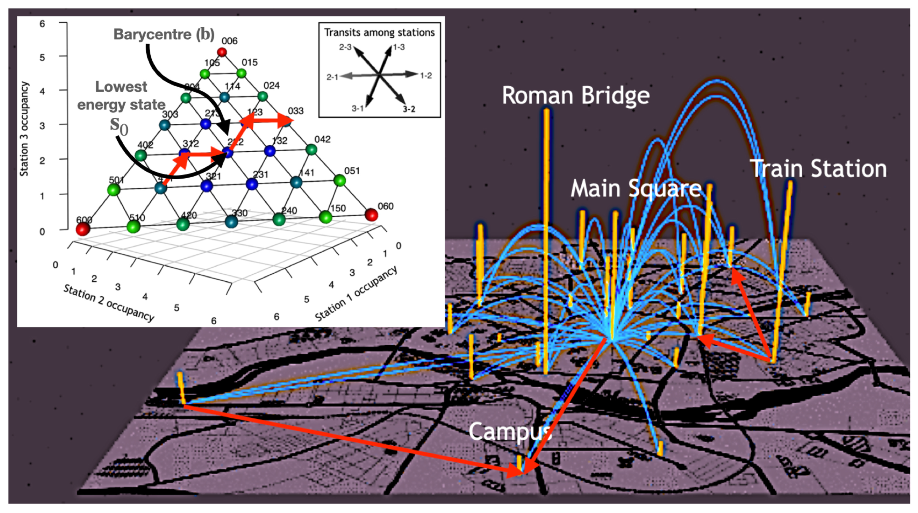
For example, for the toy model consisting of 6 units and 3 stations with capacity
, there are 28 possible arrangements (
Figure 1 inset). Since this number grows exponentially with
D and
N, the state space must be explored by heuristic methods.
Trips originated at station
i with occupancy
to station
j with occupancy
are then modelled as directed links
in the simplex (
Figure 1 inset). This way, a trip increases the number of units at destination
j by one unit while it decreases the available vehicles at the origin
i by one unit. The corresponding change of system state in the simplex can be described as
where
are the components of the D-dimensional flow vector
. The transition is defined as valid (possible) when the two following conditions hold:
Note that a valid transition corresponds to a mapping between one state
and another state
in its neighbourhood in the simplex
. This neighbourhood is defined as the points that are at a distance less or equal to
:
For example, starting from the state
, there are two valid transitions. One is
(going from station 2 to station 1), which corresponds to
, and the other one is
(going from station 2 to station 3), which corresponds to
. Our model also captures non-possible trips since a transition like
would pretend to bring a unit from station 1 (that is empty) to station 2 (which is also full). This non-possible transition would lead to a state outside the simplex as can be seen in the
Figure 1 inset. Therefore, the simplex has the property of being a set of valid states in which the motions are continuous. It should be remarked that only a certain subset of
transitions are allowed due to the boundary limit states.
Notice also that states located far from the simplex centre will tend to fall into imbalance more easily. This is because the vehicle system is balanced when station occupancy is close to 50%. This maximizes the likelihood that units will be available and that there will be space to leave a unit. This model allows us to quantify the imbalance of the state
as its distance to the barycentre of the simplex. We can further exploit the analogy with a physical system by defining the energy of a state as
, where
is the simplex barycentre. Note that
need not be a state of the simplex (see
Figure 1 inset). The idea is that points near the barycentre are more balanced and therefore have lower energy. Note that for a valid transition
we have an energy change:
In this setting, the equi-energetic surfaces correspond to states lying at equal distance from the simplex barycentre. This way, self-journeys or loops have zero energy change.
Moreover, through the equivalence relation
, it is possible to partition the simplex into macro-states. These macrostates are thus the equal-balanced surfaces in the quotient set
as defined in [
18]. A schematic of the system dynamics is shown in
Figure 1: flows among stations (arcs) are mapped to a walk in the simplex (inset). Since these flows are not symmetrical, the system tends to destabilize. This figure also shows the loops that have no energy change in the simplex depicted as vertical bars.
The lowest energy state
is the one closest to the simplex barycentre:
. Hence the lowest energy of the system is
Since is the closest state to , this configuration corresponds to balancing the load of all stations in the network with a number of units close to .
In the opposite case, the imbalance occurs when stations are filled to their limit and others remain empty. By performing the integer division
for
and
, a typical unbalanced state will be of the form given in Equation (
7).
This corresponds to
Q stations with their maximum occupancy,
C,
stations being completely empty and one station with occupancy
r, being the energy of this state:
Note that permutations among the s components produce the same energy. The maximum is obtained for states in which : . Note that by construction, the states closest to collapse are on the simplex boundary. These states are only one transition away from producing the collapse of the system.
Notice also that the simplex model only gives sufficient conditions for the system to “collapse”, where collapse is understood to be a lack of service due to a station being either empty when one intends to purchase a vehicle or full when one intends to deposit their vehicle. It is clear that the system can collapse for many other reasons not considered in our model (e.g., closing of stations or other enforced external actions).
3. Asymmetry and Super Diffusion: The Effect of Self-Journeys (Loops)
Based on the model defined above, we inquire how spatio-temporal asymmetries in the distribution of stations and users’ schedules create different mobility patterns and how these latter contribute to the overall system collapse. To do so, we start from a set of 17,000 trips stored as time-stamped origin–destination records. The data were collected in the period 2014–2017 in the city of Salamanca (Spain). There are 29 stations and as found in [
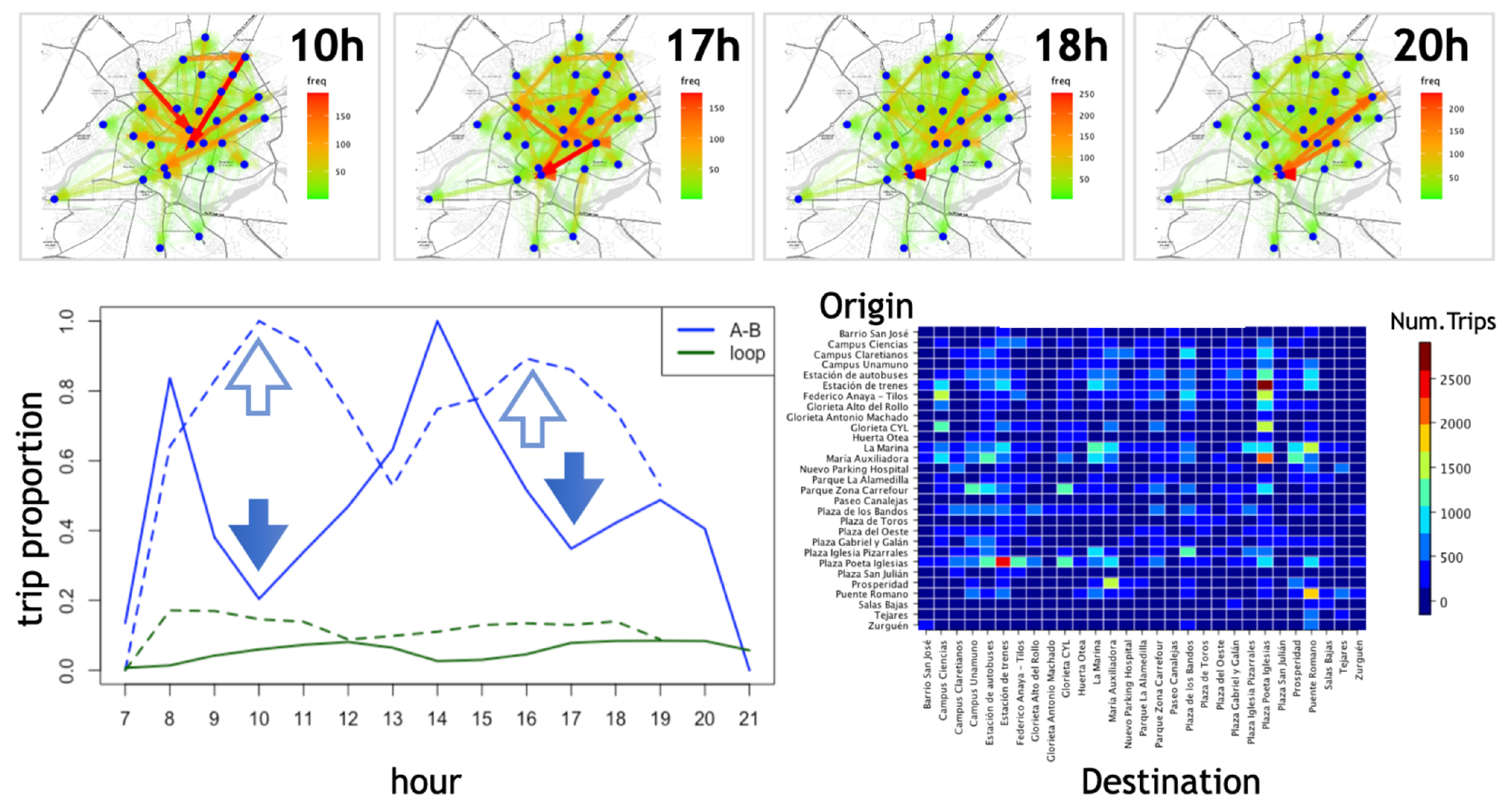
7], we observe in
Figure 2 a trimodal pattern of mobility correlated to the daily working activity.
Notice however that the trimodal pattern of A–B trips during workdays shifts to a a bimodal pattern on the weekend. Additionally, self-journeys of the form A–A (in this paper referred to simply as 1-trip loops or loops) have a bimodal pattern for both workdays and weekends. The reason is that loops have a different dynamic than A–B workday trips but are not so different than A–B journeys during weekends. This is likely caused by different user profiles who have different priorities (e.g., on weekends, people do not need to commute at lunchtime and so the central peak disappears).
A global portrait of the movements at different times can be obtained by monitoring the flows at different timestamps (
Figure 2 Top). To do this, at a given time, we extract the trips and sort them by frequency. Then, we generate a uniform distribution between 1 and the maximum number of trips for each hour. Then, we choose the paths with a frequency greater than 50% of the paths in that hour (in
Figure 2, we only present the hours with the highest incidence as the others have less striking patterns). Loops represent only 6.47% of the trips, but as we will see below, they play an important role. Notice the organized activity at 20 h compared to the more chaotic-like pattern at 17 h.
In
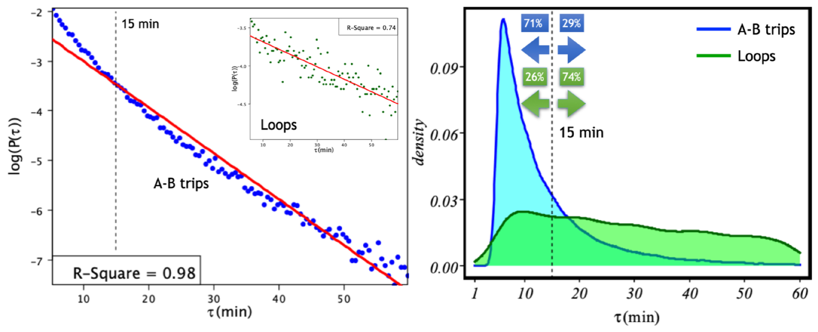
Figure 3, we show the inter-arrival time (IAT) distribution for both A–B trips and loops for the fleet of 29 bike-sharing stations in the city of Salamanca. Firstly, we notice that for the case of A–B trips (
Figure 3 left), a fit to a Poisson distribution
seems to reveal the existence of two time scales: one corresponding to trips shorter than 15 min and another scale corresponding to trips of larger times. This effect is not observed for self-journeys (
Figure 3 left inset), although in this case, the fitting is weaker (
). To further clarify whether loops are responsible for the two-scales effect not captured by the Poisson model in
Figure 3 right, we analyse the distributions of both types of trips. There, we notice that loops have a much longer tail than A–B trips and that most self-journeys (
) correspond to longer times. This rules out the possibility that loops are responsible for the two observed time scales. Although it is very interesting to delve into the reasons for this division of scales, this would take us too far in this first work, and we leave its analysis for future work. The fitted rates for A–B trips and loops are
min ≈ 1 event per 10 min (A-B trips) and
min ≈ 1 events per hour (loops).
On the other hand, loops produce no net change in the balance of units in the stations. Thus, loops must play an important role in the dynamics of the system. Clearly, the complexity of the dynamics arises from the spatial distribution of the stations, the temporal patterns of the users and the correlation of these two factors with the number of loops. In this respect, we ask three questions: (1) how to compare the movements in the simplex with respect to random walks, (2) how to characterise the complexity of the system, and (3) how to quantify the expected collapse time. Let us first look at what a diffusion process in the simplex looks like.
The
walk in the simplex is constructed by iterating Equation (
3) for
n steps:
with
being simple random variables taking values
. By assuming
, energies can be calculated as follows (If the first state is not exactly the barycentre, there is only one correction as an additive constant):
However, noticing that
—this holds from the definition of
—the mean value of the energy is as follows:
The super-diffusive term will be 0 for purely random motions. In this case, we obtain
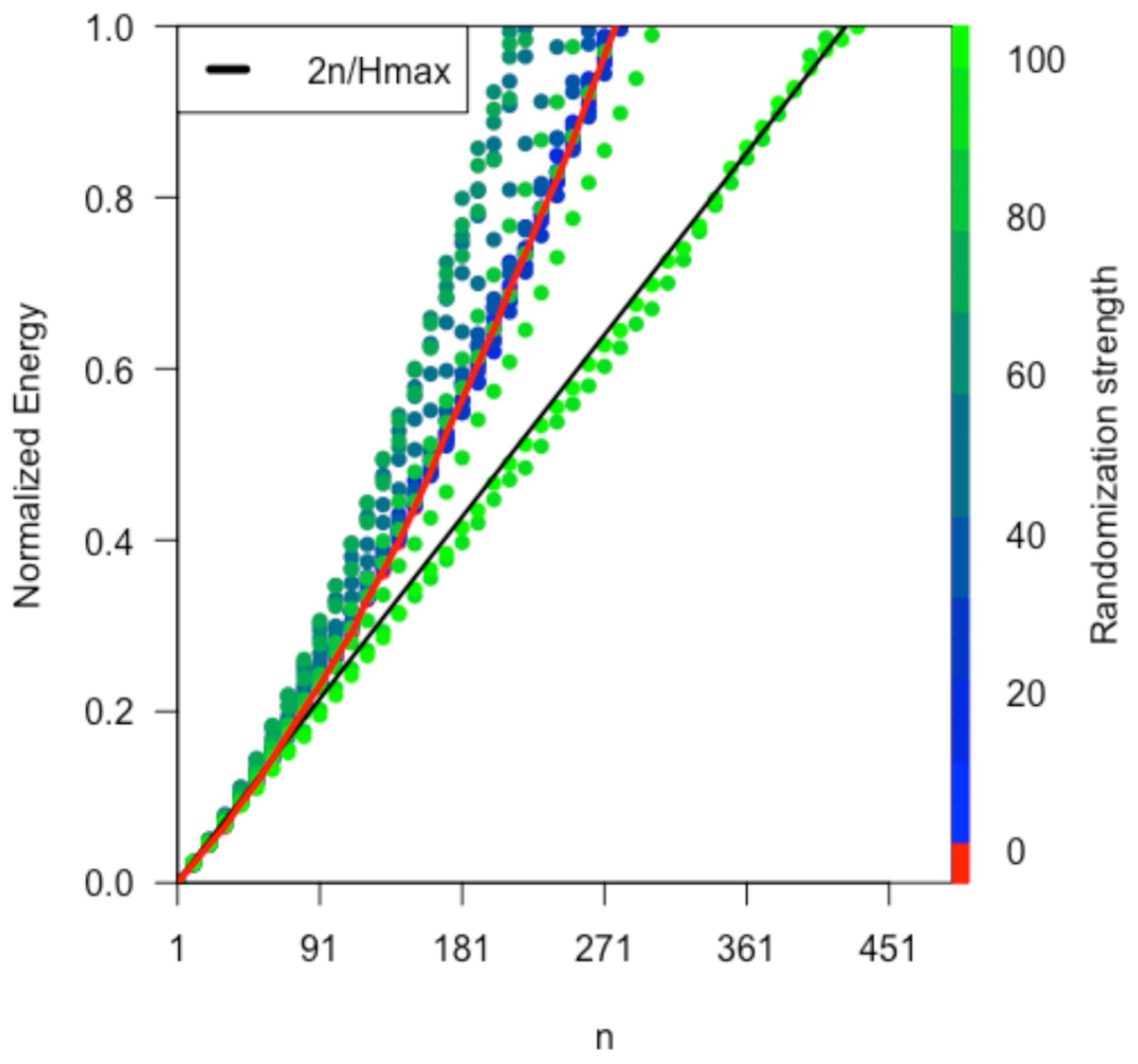
. However, the presence of non-symmetric flows renders higher diffusive behaviour. To check this, we compare the diffusion in the observed trips with random walks by simulating walks starting from a state near
and driven by the empirical probabilities
corresponding to a
trip. Furthermore, we increasingly randomize the
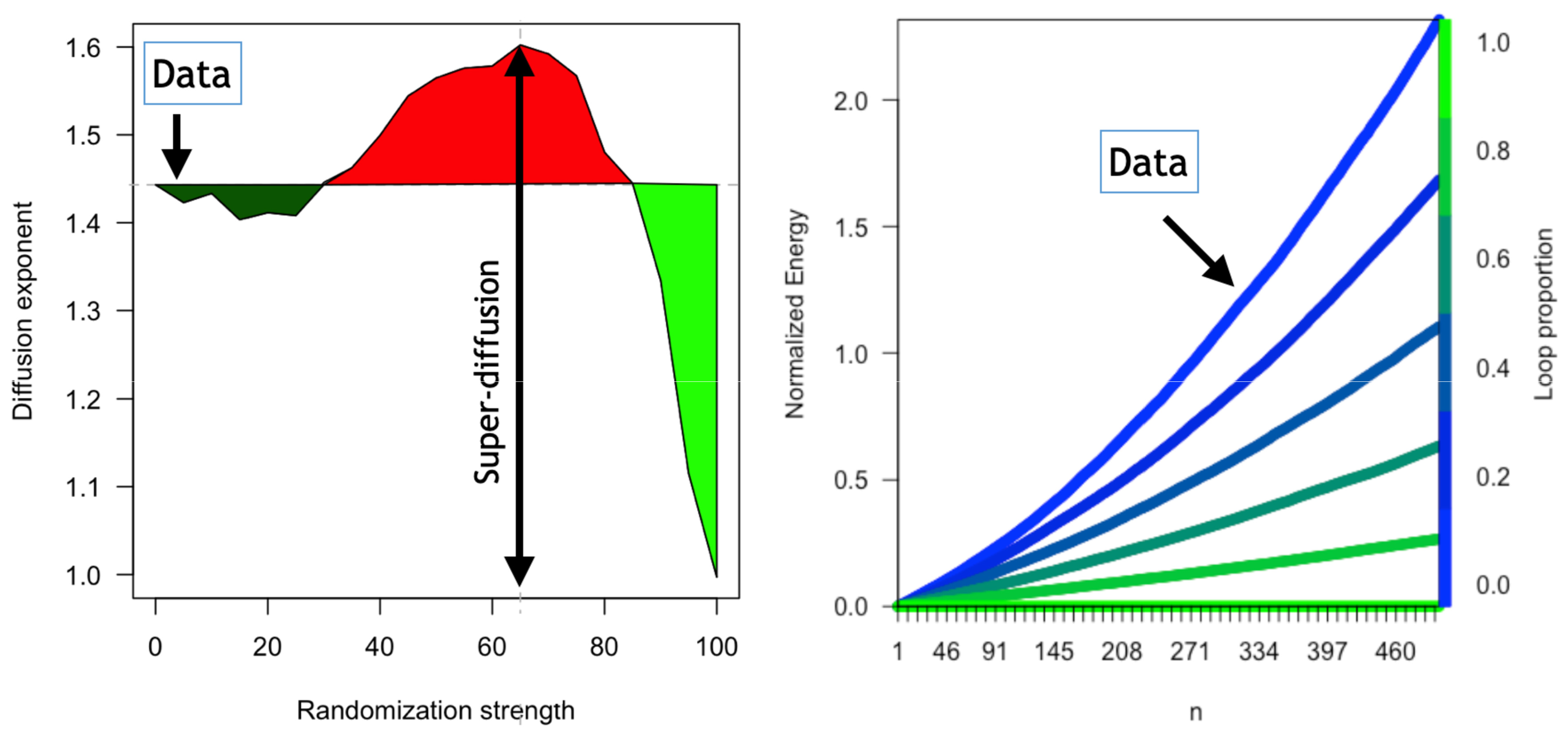
weights and monitor the effect. We then plot the normalized energy in the simplex for each iteration as shown in
Figure 4. We describe this process in detail in the
Supplementary Material.
By fitting the curves for each power law of the form,
where
n is the number of steps, we have also calculated the diffusion exponents (
Figure 5 left) for each randomization level. Note that, as we increase the percentage of random trips, three phases appear:
<30% random trips: diffusion is less rapid than that found in the data ().
30–90% random trips: the super-diffusive regime spreads faster than that observed in the data and peaks at for .
>90% random trips (near total random): the super-diffusion drops abruptly, and the system starts to diffuse as a random walk in which the normalized energy (unbalance) grows linearly with n and .
On the other hand, in
Figure 5 right, we monitor the normalized energy as the proportion of loops in the data grows. As noticed, loops slow down the diffusion and when all trips become loops, there is no diffusion at all.
Figure 5 also shows how the system naturally overdiffuses for real data and that in general external mechanisms are necessary to rebalance the system, as it is common in shared mobility.
The asymmetric drift present in the empirical
(
Figure 2 bottom right) causes the observed super-diffusion, and we conjecture that the macroscopic effect of this mechanism must also have an origin in the long correlations caused by interactions within the system.
4. Measuring System’s Complexity: Multi-Scale Entropy and Complexity Profile
To gain more insight into the cause of the observed anomalous diffusion, we quantitatively characterise the complexity of the system. The long-range correlations create a persistence of structures on a temporal scale. Firstly, Refs. [
19,
20] propose the approximate entropy (
ApEn) as a measure of changes in the complexity of a system. This metric offers greater robustness than others previously used, and requires a much smaller number of observations.
ApEn measures the (logarithmic) likelihood that runs of patterns that are close remain close upon next incremental comparisons. For ordered series, a value of
ApEn close to 0 means that patterns persist on an immediately larger scale, which is typical of a deterministic system.
Later on, [
21] extended the
ApEn metric to sample entropy (
SampEn) from shortcomings observed in heart rate dynamics. This new measure avoids self-matching in the patterns, resulting in a more reliable estimation, especially when the number of samples is small.
Following the notation of [
19], let us consider
N temporally ordered observations with points
. The idea now is to form vectors with
m consecutive points, starting from a position
i in the series:
, with
. Then, for each
i, given a threshold
r, the following quantities are computed:
: number of vectors such that the distance lies below threshold r.
: same as but using -sized vectors instead of vectors of length m.
Then, according to [
21], we define the sample entropy,
, as
Notice that sampEn is just the negative logarithm of an estimate of the conditional probability of a match between vectors given a match of the m-sized vectors. Thus, the sampEn searches for the probability of a larger pattern, given a pattern of order m. Usually, the values and are used.
It is worth mentioning that the concept of
has been extended to other fields, such as, for example, to the study of physiological time series [
22,
23] (a systematic review of the multiscale entropy algorithm and its variants is given in [
24]). The authors identified the need to introduce a complexity metric more appropriate to biological systems in which a loss of complexity may be a generic feature of pathologic dynamics. This new measure would take into account the fact that complex systems might process information differently depending on the scale. The idea is to quantify the information conveyed over multiple scales. To this end, multi-scale entropy (MSE) [
22] can be defined as the computation of
SampEn for different coarse-grained versions of the series. That is, if we have scales
, we create the vectors
As it is well known, chaotic signals [
25,
26] usually have a memoryless white noise pattern. However, complex systems often present series with
-type noise that manifests correlations between spatio-temporal scales. The authors of [
22] use the MSE and find that the multi-scale entropy of arterial fibrillated patients (as in the case of white noise signals) drops rapidly with increasing scale, but the entropy of healthy individuals (such as
noise) remains almost constant across different scales. This behaviour makes the MSE a more reliable metric for identifying complexity than the simple computation of
SampEn at one particular scale.
In our case, instead of a numerical time series, we have a chain of source–destination pairs of the form
. Hence, we must modify the sums of Equation (
14). A convenient way to perform this aggregation is to choose the most frequent (i.e., the mode) trip
in the corresponding portion of the coarse-grained time series. Thus, we implement MSE as follows:
In addition, to calculate the inter-path distances required to compute the
SampEn, we use the Jaccard distance given by
where
and
. Notice that with this definition, trips (i.e., loops) of the form
have distance 0, while the distance between trips
and
is 1. In the
Supplementary Material, we show the pseudocode for the explicit construction of the
SampEn and MSE metrics, respectively.
In
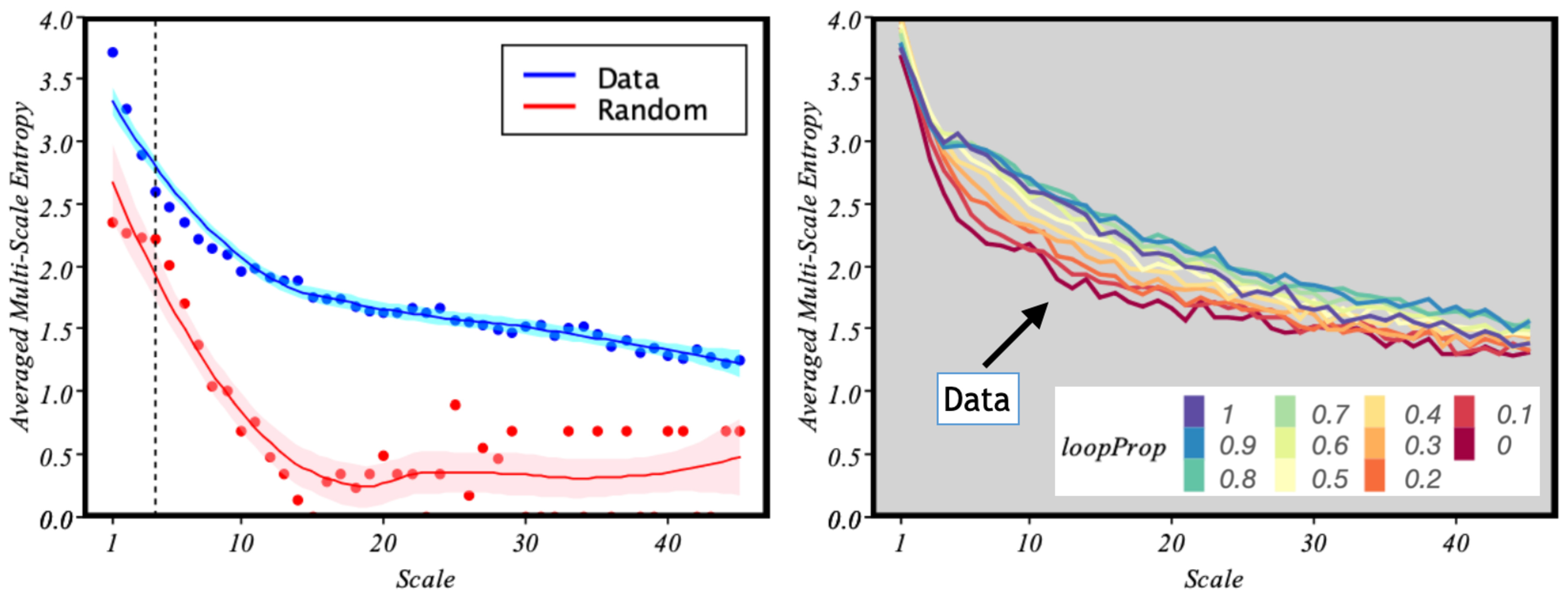
Figure 6, we present the MSE of the data against a randomized situation in which
trips are chosen randomly for parameters
and
. Note that the MSE soon drops rapidly for the random case, but it decreases smoothly in the case of the empirical data series. This effect was observed by Costa et al. [
22] when they compared the MSE for white noise and
noise.
In particular, notice also (
Figure 6 left) how for a scale around 4, which, according to the event rate
one event every 10 min (found in
Section 3), the MSE of the data is close to that of the random case. Such a scale roughly corresponds to 40 min. From that threshold, a random system would quickly lose information between time scales. However, in the case of urban mobility, the information transmitted between scales is maintained, which is a proxy for self-organisation and complexity.
Furthermore, in
Figure 5 (right), we saw that the loops have a stabilising effect by decreasing the energy of the system. Based on
Figure 6 right, we see that this result is consistent. Indeed, if we gradually introduce artificial loops into the data, we see that in general, increasing the number of loops makes the behaviour of the system more correlated. Interestingly, the maximum number of loops—
—does not make the system more organised, as there seems to be a threshold at
.
Finally, we will use a concept that has proven to be useful for characterising complex systems: the complexity profile [
27]. Given a metric of complexity—in our case, we postulate the MSE as a good candidate—the complexity profile simply plots the value of the metric as a function of scale. A complex system is expected to maintain high values of the metric for large scales. Here, we define our complexity profile as the area under the curve (AUC) of the MSE. Consequently, the complexity profile of the data drops much more smoothly than the randomized samples as shown in
Figure 7.
In
Figure 7, we present the complexity profile. First of all, we can see how this metric is able to separate more clearly the complex behaviour from that of an equivalent random system, as it is more robust under noise
Figure 7 left. On the other hand, the complexity profile is also consistent with the role that loops play in the system (right). Self-journeys contribute to increasing the long-range correlations. However, they do so in a way that decreases diffusion and therefore contributes to stabilising the system.
6. Conclusions
The first goal of the paper was to unveil the collapse conditions of a network of shared mobility vehicles. To do so, we built and explored a network of stations with limited capacity through which users commute in shared vehicles. We showed how the dynamics of the system is determined by non-random walks in a certain state space (simplex). In this space, by using statistical physics techniques, it is possible to understand the imbalance of the system in terms of energy, which provides a valuable insight into the diffusion mechanisms. We found that the system tends to collapse naturally over time (which was reported in the highlighted results). In particular, the diffusion is anomalous because the asymmetry of travel trends creates diffusions that are not balanced in different areas of the city. This result explains why an additional external rebalancing mechanism is necessary to keep the system in equilibrium. Furthermore, we gave analytical expressions for the collapse probability and for the super-diffusion exponents.
In light of our model, self-journeys (i.e., loops), although being a small proportion of the total trips, play an important role in the stabilization of the system. The reason is that loops produce no net energy shift in the simplex. Both multiscale entropy and complexity profile techniques have been applied to real data from a bicycle sharing fleet in the city of Salamanca (Spain). The results have shown that the system presents a complexity behaviour that shows self-organisation, which is far from random white noise. This fact is relevant since complex systems are known to have other properties, such as robustness and adaptability. These results can be directly extrapolated to other car-sharing systems.
Furthermore, we believe that our work can be extended in the future to find the seasons and times at which loops have the greatest impact on system stability. These results would help to design mobility policies that promote self-journeys at specific times and in specific areas to maintain system saturation with minimal external intervention. In particular, we characterise the dynamic system and the associated stochastic processes in a way that is independent of the type of vehicles, stations, etc.
It should be noted that our model is limited by the fact that we have neglected many other effects that could lead to system collapse (traffic congestion, loss of vehicles, etc.). However, our analysis, by not taking into account all of these additional factors, provides a conservative limit when investigating a possible real collapse.
To conclude, in future work, we will investigate networks of stations of different capacities as well as the effect of traffic in the system dynamics.
