
Variational Bayesian Inference for Nonlinear Hawkes Process with Gaussian Process Self-Effects


Abstract
:1. Introduction
Outline
2. Proposed Model
2.1. Classical Hawkes Process
2.2. Nonlinear Hawkes Process with Gaussian Process Self-Effects
Multivariate Model
3. Inference
3.1. Model Augmentation
3.2. Variational Inference
3.3. Optimal
3.4. Optimal
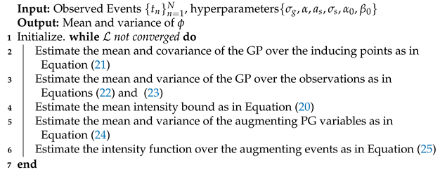
| Algorithm 1: NH–GPS Variational Inference. |
 |
Hyperparameters Tuning
3.5. Identifying the Background Rate and the Self-Effects Function
4. Related Work
5. Experiments
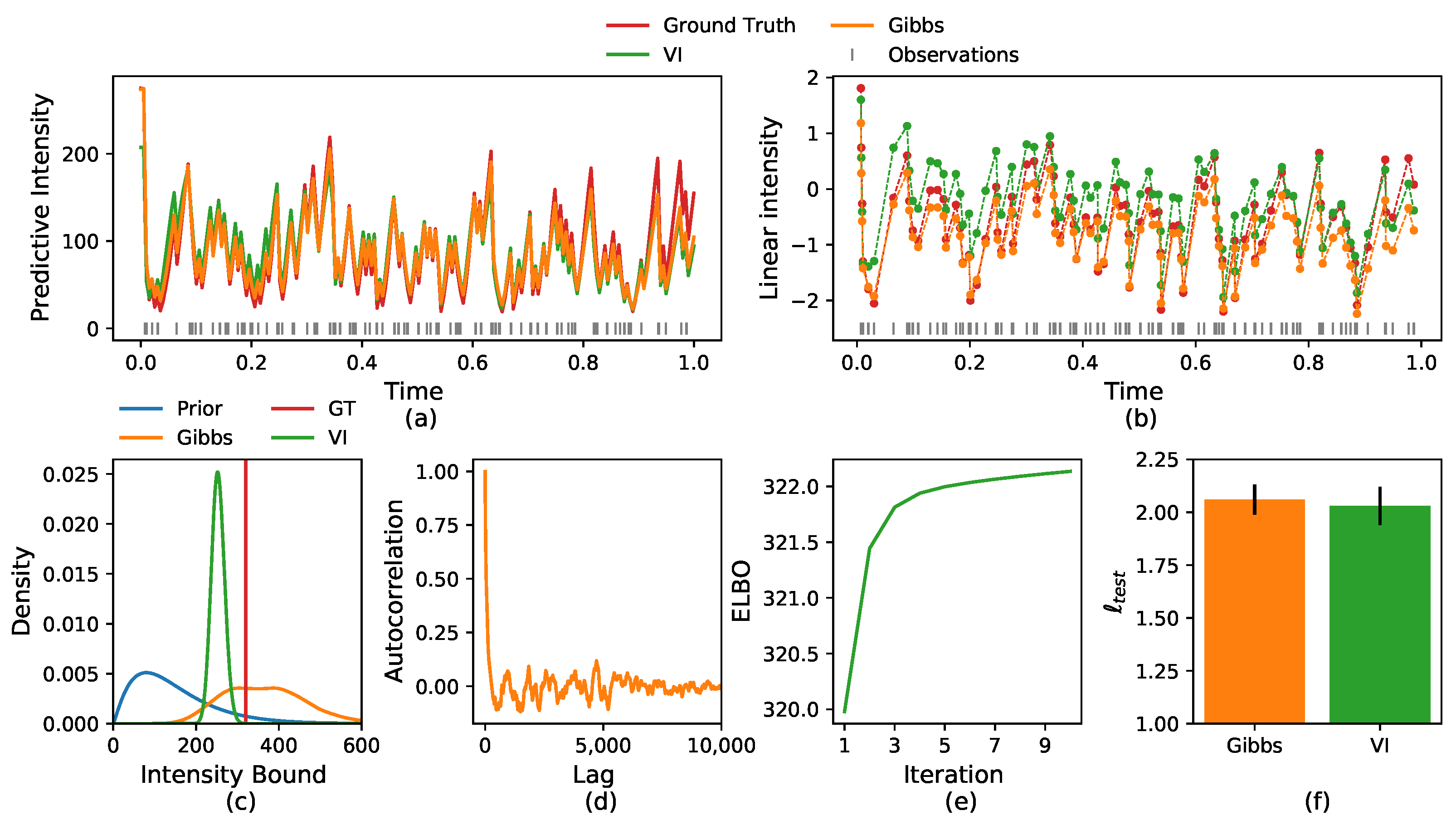
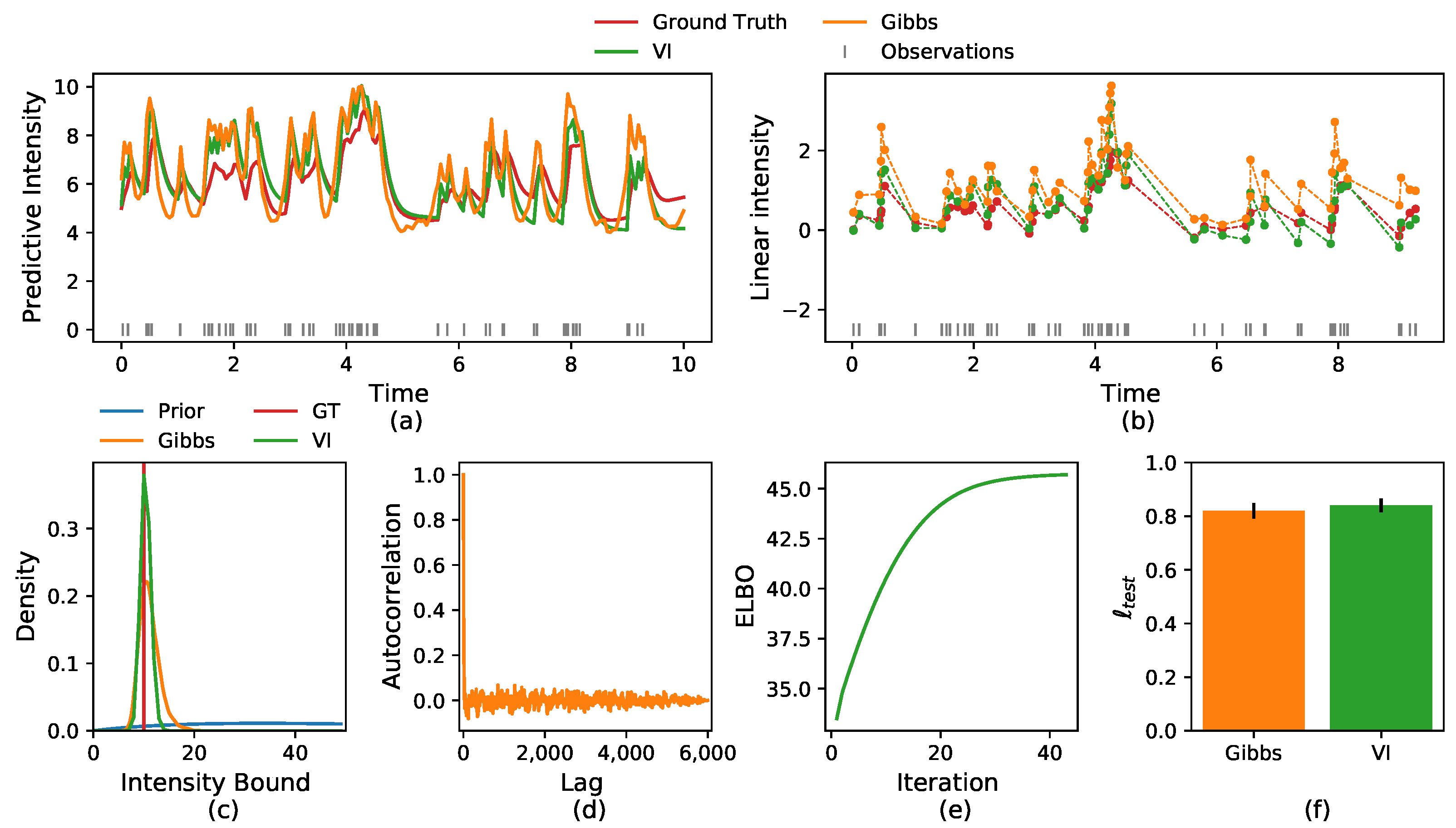
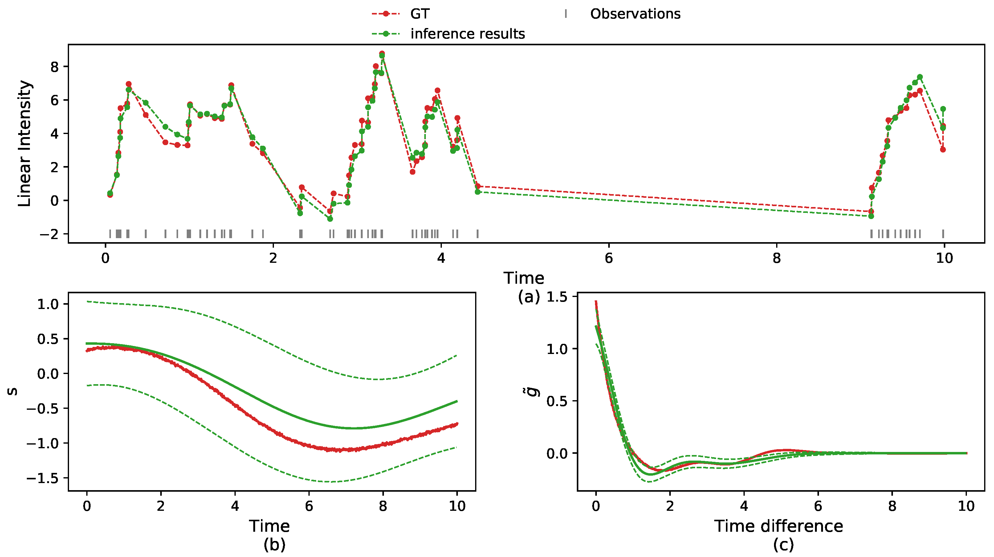
5.1. Synthetic Data
5.2. Real Data
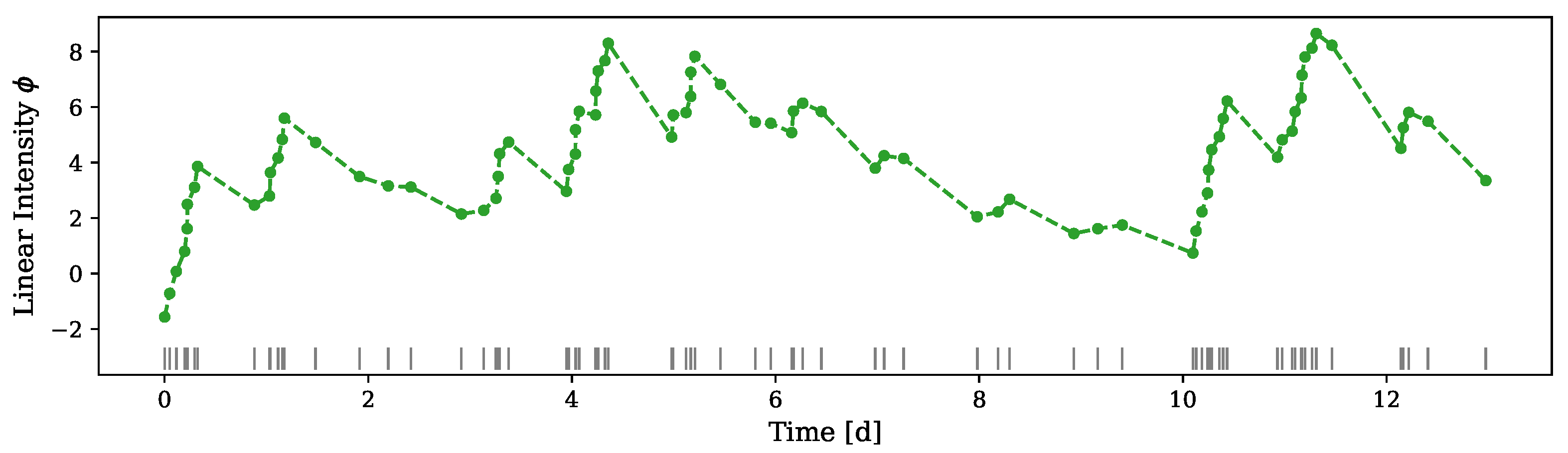
5.2.1. Crime Report Data
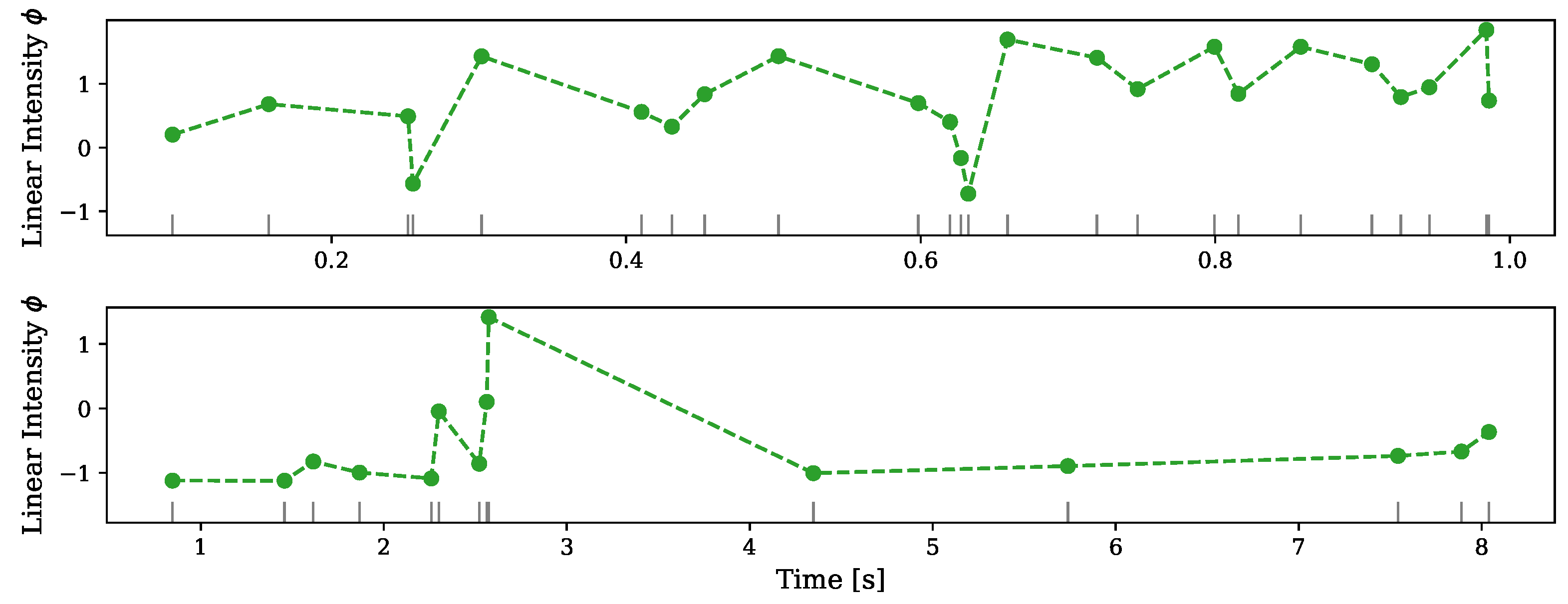
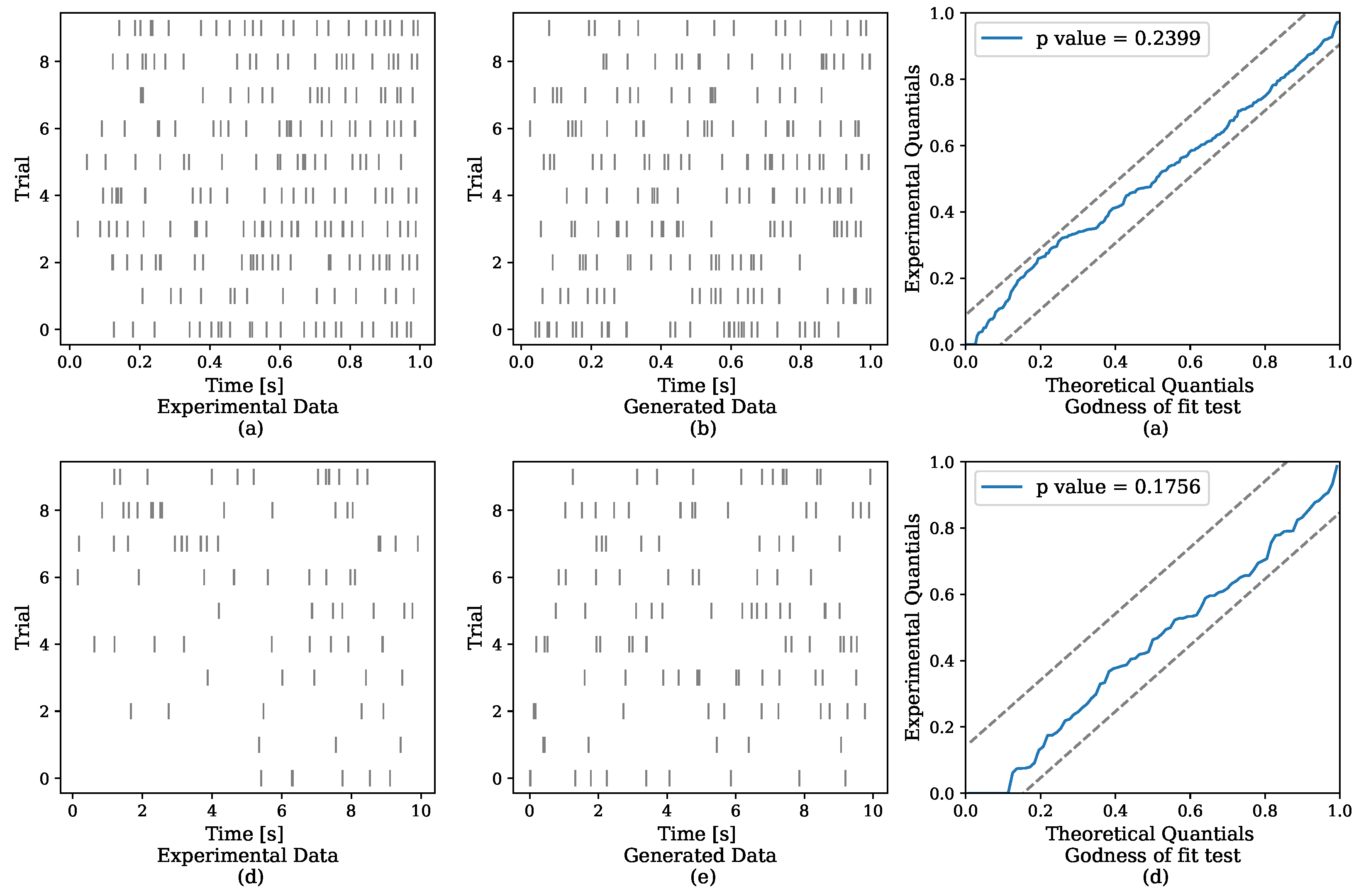
5.2.2. Neuronal Activity Data
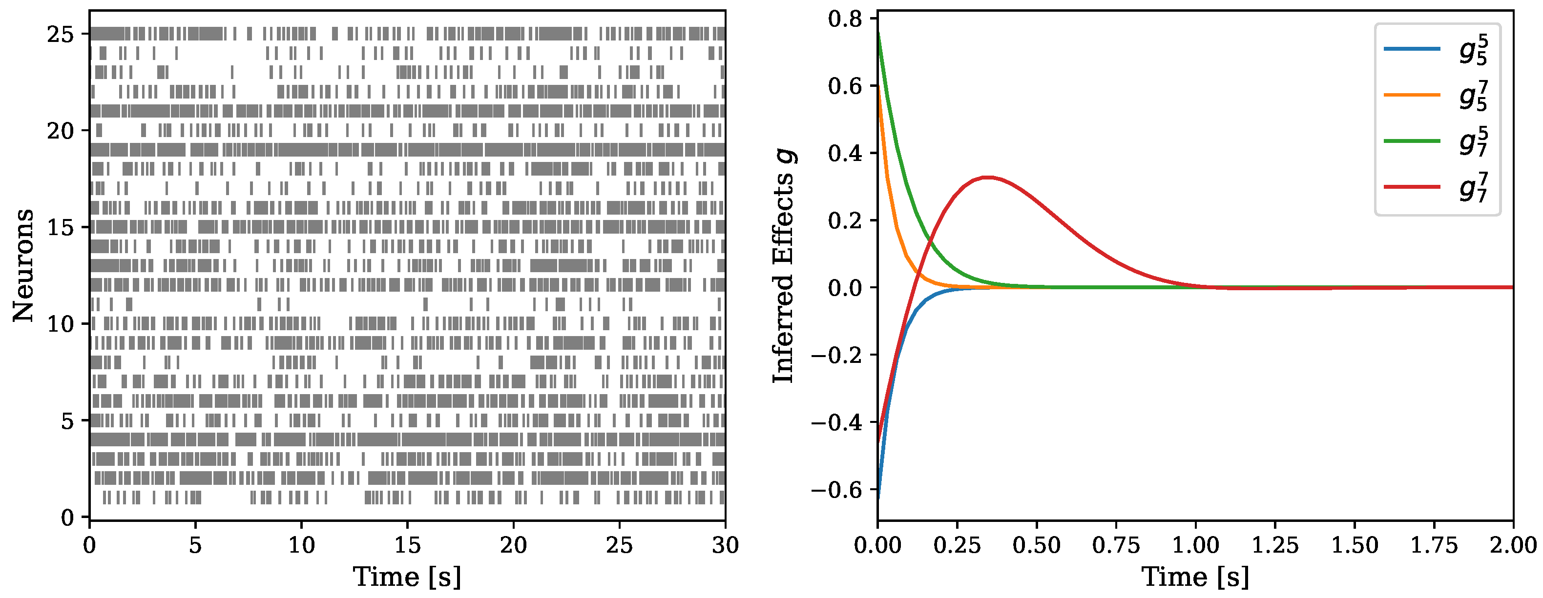
5.2.3. Multi-Neurons Data
6. Discussion
Author Contributions
Funding
Data Availability Statement
Acknowledgments
Conflicts of Interest
Appendix A. Gibbs Sampler
Appendix A.1. Conditional Distribution of the Upper Intensity Bound
Appendix A.2. Conditional Distribution of the Linear Intensity Function
Appendix A.3. Conditional Distribution of the PG Variables
Appendix A.4. Conditional Distribution of the Augmenting Events
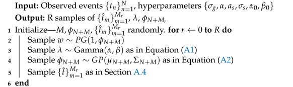
| Algorithm 2: NH–GPS Gibbs Sampler |
 |
Appendix B. Hyperparameters Learning for the Gibbs Sampler
References
- Ogata, Y. Statistical models for earthquake occurrences and residual analysis for point processes. J. Am. Stat. Assoc. 1988, 83, 9–27. [Google Scholar] [CrossRef]
- Zhao, Q.; Erdogdu, M.A.; He, H.Y.; Rajaraman, A.; Leskovec, J. SEISMIC: A Self-Exciting Point Process Model for Predicting Tweet Popularity. In Proceedings of the 21st ACM SIGKDD International Conference on Knowledge Discovery and Data Mining; Association for Computing Machinery (KDD ‘15), New York, NY, USA, 10–13 August 2015; pp. 1513–1522. [Google Scholar]
- Dayan, P.; Abbott, L.F. Theoretical Neuroscience: Computational and Mathematical Modeling of Neural Systems; MIT Press: Cambridge, MA, USA, 2001; Chapter 7.5; pp. 265–273. [Google Scholar]
- Cox, D.R. Some statistical methods connected with series of events. J. R. Stat. Soc. Ser. B 1955, 17, 129–157. [Google Scholar] [CrossRef]
- Hawkes, A.G.; Oakes, D. A cluster process representation of a self-exciting process. J. Appl. Probab. 1974, 11, 493–503. [Google Scholar] [CrossRef]
- Maffei, A.; Nelson, S.B.; Turrigiano, G.G. Selective reconfiguration of layer 4 visual cortical circuitry by visual deprivation. Nat. Neurosci. 2004, 7, 1353–1359. [Google Scholar] [CrossRef]
- Smith, T.C.; Jahr, C.E. Self-inhibition of olfactory bulb neurons. Nat. Neurosci. 2002, 5, 760–766. [Google Scholar] [CrossRef]
- Brémaud, P.; Massoulié, L. Stability of nonlinear Hawkes processes. Ann. Probab. 1996, 1563–1588. [Google Scholar] [CrossRef]
- Zhu, L. Central limit theorem for nonlinear Hawkes processes. J. Appl. Probab. 2013, 50, 760–771. [Google Scholar] [CrossRef]
- Truccolo, W. From point process observations to collective neural dynamics: Nonlinear Hawkes process GLMs, low-dimensional dynamics and coarse graining. J. Physiol. 2016, 110, 336–347. [Google Scholar] [CrossRef]
- Sulem, D.; Rivoirard, V.; Rousseau, J. Bayesian estimation of nonlinear Hawkes process. arXiv 2021, arXiv:2103.17164. [Google Scholar]
- Jia, J.; Benson, A.R. Neural jump stochastic differential equations. arXiv 2019, arXiv:1905.10403. [Google Scholar]
- Xiao, S.; Farajtabar, M.; Ye, X.; Yan, J.; Song, L.; Zha, H. Wasserstein Learning of Deep Generative Point Process Models. In Advances in Neural Information Processing Systems; Guyon, I., Luxburg, U.V., Bengio, S., Wallach, H., Fergus, R., Vishwanathan, S., Garnett, R., Eds.; Curran Associates, Inc.: Long Beach, CA, USA, 2017; Volume 30. [Google Scholar]
- Kingman, J.F.C. Poisson Processes; Oxford Studies in Probability Volume 3; The Clarendon Press Oxford University Press: New York, NY, USA, 1993. [Google Scholar]
- Daley, D.J.; Vere-Jones, D. An Introduction to the Theory of Point Processes: Volume II: General Theory and Structure; Springer Science & Business Media: Berlin/Heidelberg, Germany, 2007. [Google Scholar]
- Rasmussen, J.G. Bayesian inference for Hawkes processes. Methodol. Comput. Appl. Probab. 2013, 15, 623–642. [Google Scholar] [CrossRef] [Green Version]
- Zhou, F.; Li, Z.; Fan, X.; Wang, Y.; Sowmya, A.; Chen, F. Efficient Inference for Nonparametric Hawkes Processes Using Auxiliary Latent Variables. J. Mach. Learn. Res. 2020, 21, 1–31. [Google Scholar]
- Daley, D.J.; Vere-Jones, D. An Introduction to the Theory of Point Processes: Volume I, 2nd ed.; Probability and Its Applications; Springer: New York, NY, USA, 2003. [Google Scholar]
- Donner, C.; Opper, M. Efficient Bayesian inference of sigmoidal Gaussian Cox processes. J. Mach. Learn. Res. 2018, 19, 2710–2743. [Google Scholar]
- Apostolopoulou, I.; Linderman, S.; Miller, K.; Dubrawski, A. Mutually Regressive Point Processes. In Advances in Neural Information Processing Systems; Wallach, H., Larochelle, H., Beygelzimer, A., d’Alché-Buc, F., Fox, E., Garnett, R., Eds.; Curran Associates, Inc.: Vancouver, BC, Canada, 2019; Volume 32. [Google Scholar]
- Polson, N.G.; Scott, J.G.; Windle, J. Bayesian inference for logistic models using Pólya–Gamma latent variables. J. Am. Stat. Assoc. 2013, 108, 1339–1349. [Google Scholar] [CrossRef] [Green Version]
- Donner, C.; Opper, M. Efficient Bayesian Inference for a Gaussian Process Density Model. In Proceedings of the Conference on Uncertainty in Artificial Intelligence, Monterey, CA, USA, 6–10 August 2018; Globerson, A., Silva, R., Eds.; PMLR; AUAI Press: Monterey, CA, USA, 2018. [Google Scholar]
- Jordan, M.I.; Ghahramani, Z.; Jaakkola, T.S.; Saul, L.K. An introduction to variational methods for graphical models. Mach. Learn. 1999, 37, 183–233. [Google Scholar] [CrossRef]
- Bishop, C.M. Pattern Recognition and Machine Learning; Springer: New York, NY, USA, 2006. [Google Scholar]
- Csató, L.; Opper, M.; Winther, O. TAP Gibbs Free Energy, Belief Propagation and Sparsity. In Proceedings of the Neural Information Processing Systems: Natural and Synthetic (NIPS), Vancouver, BC, Canada, 3–8 December 2001; pp. 657–663. [Google Scholar]
- Titsias, M.K. Variational Learning of Inducing Variables in Sparse Gaussian Processes. In JMLR Proceedings, Proceedings of the International Conference on Artificial Intelligence and Statistics, Clearwater Beach, CA, USA, 16–18 April 2009; Dyk, D.A.V., Welling, M., Eds.; PMLR: Birmingham, UK, 2009; Volume 5, pp. 567–574. [Google Scholar]
- Hensman, J.; Matthews, A.G.d.G.; Filippone, M.; Ghahramani, Z. MCMC for variationally sparse Gaussian processes. arXiv 2015, arXiv:1506.04000. [Google Scholar]
- Lloyd, C.M.; Gunter, T.; Osborne, M.A.; Roberts, S.J. Variational Inference for Gaussian Process Modulated Poisson Processes. In JMLR Workshop and Conference Proceedings, Proceedings of the International Conference on Machine Learning, Lille, France, 6–11 July 2015; Bach, F.R., Blei, D.M., Eds.; PMLR: Birmingham, UK, 2015; Volume 37, pp. 1814–1822. [Google Scholar]
- Møller, J.; Syversveen, A.R.; Waagepetersen, R.P. Log gaussian cox processes. Scand. J. Stat. 1998, 25, 451–482. [Google Scholar] [CrossRef]
- Brix, A.; Diggle, P.J. Spatiotemporal prediction for log-Gaussian Cox processes. J. R. Stat. Soc. Ser. B 2001, 63, 823–841. [Google Scholar] [CrossRef]
- Adams, R.P.; Murray, I.; MacKay, D.J.C. Tractable nonparametric Bayesian inference in Poisson processes with Gaussian process intensities. In ACM International Conference Proceeding Series, Proceedings of the 26th Annual International Conference on Machine Learning, Montreal, QC, Canada, 14–18 June 2009; Danyluk, A.P., Bottou, L., Littman, M.L., Eds.; ACM: New York, NY, USA, 2009; Volume 382, pp. 9–16. [Google Scholar]
- Ishwaran, H.; James, L.F. Computational methods for multiplicative intensity models using weighted gamma processes: Proportional hazards, marked point processes, and panel count data. J. Am. Stat. Assoc. 2004, 99, 175–190. [Google Scholar] [CrossRef]
- Wolpert, R.L.; Ickstadt, K. Poisson/gamma random field models for spatial statistics. Biometrika 1998, 85, 251–267. [Google Scholar] [CrossRef] [Green Version]
- Taddy, M.A.; Kottas, A. Mixture modeling for marked Poisson processes. Bayesian Anal. 2012, 7, 335–362. [Google Scholar] [CrossRef]
- Zhang, R.; Walder, C.; Rizoiu, M.A.; Xie, L. Efficient non-parametric Bayesian Hawkes processes. arXiv 2018, arXiv:1810.03730. [Google Scholar]
- Zhou, F.; Li, Z.; Fan, X.; Wang, Y.; Sowmya, A.; Chen, F. Efficient EM-Variational Inference for Hawkes Process. arXiv 2019, arXiv:1905.12251. [Google Scholar] [CrossRef]
- Zhang, R.; Walder, C.J.; Rizoiu, M.A. Variational Inference for Sparse Gaussian Process Modulated Hawkes Process. In Proceedings of the AAAI Conference on Artificial Intelligence, New York, NY, USA, 7–12 February 2020; AAAI Press: Palo Alto, CA, USA, 2020; pp. 6803–6810. [Google Scholar]
- Zhou, F.; Zhang, Y.; Zhu, J. Efficient Inference of Flexible Interaction in Spiking-neuron Networks. In Proceedings of the 9th International Conference on Learning Representations (ICLR 2021), Vienna, Austria, 3–7 May 2021. [Google Scholar]
- Bradbury, J.; Frostig, R.; Hawkins, P.; Johnson, M.J.; Leary, C.; Maclaurin, D.; Necula, G.; Paszke, A.; VanderPlas, J.; Wanderman-Milne, S.; et al. JAX: Composable Transformations of Python+NumPy Programs. 2018. Available online: https://github.com/google/jax (accessed on 28 January 2022).
- Linderman, S. PyPólyaGamma. GitHub. 2017. Available online: https://github.com/slinderman/pypolyagamma (accessed on 28 January 2022).
- Lewis, P.W.; Shedler, G.S. Simulation of nonhomogeneous Poisson processes by thinning. Nav. Res. Logist. Q. 1979, 26, 403–413. [Google Scholar] [CrossRef]
- Mohler, G.O.; Short, M.B.; Brantingham, P.J.; Schoenberg, F.P.; Tita, G.E. Self-exciting point process modeling of crime. J. Am. Stat. Assoc. 2011, 106, 100–108. [Google Scholar] [CrossRef]
- Gerhard, F.; Deger, M.; Truccolo, W. On the stability and dynamics of stochastic spiking neuron models: Nonlinear Hawkes process and point process GLMs. PLoS Comput. Biol. 2017, 13, 1–31. [Google Scholar] [CrossRef] [Green Version]
- Brown, E.N.; Barbieri, R.; Ventura, V.; Kass, R.E.; Frank, L.M. The time-rescaling theorem and its application to neural spike train data analysis. Neural Comput. 2002, 14, 325–346. [Google Scholar] [CrossRef]
- Ogata, Y. On Lewis’ simulation method for point processes. IEEE Trans. Inf. Theory 1981, 27, 23–31. [Google Scholar] [CrossRef] [Green Version]
- Rasmussen, C.E.; Williams, C.K.I. Adaptive computation and machine learning. In Gaussian Processes for Machine Learning; MIT Press: Cambridge, MA, USA, 2006. [Google Scholar]
- Gilks, W.R.; Wild, P. Adaptive Rejection Sampling for Gibbs Sampling. J. R. Stat. Soc. Ser. C 1992, 41, 337–348. [Google Scholar] [CrossRef]
- Martino, L.; Yang, H.; Luengo, D.; Kanniainen, J.; Corander, J. A fast universal self-tuned sampler within Gibbs sampling. Digit. Signal Process. 2015, 47, 68–83. [Google Scholar] [CrossRef]
- Hastings, W.K. Monte Carlo sampling methods using Markov chains and their applications. Biometrika 1970, 57, 97–109. [Google Scholar] [CrossRef]
- Duane, S.; Kennedy, A.D.; Pendleton, B.J.; Roweth, D. Hybrid Monte Carlo. Phys. Lett. B 1987, 195, 216–222. [Google Scholar] [CrossRef]

| Dataset | Zhou et al. (2020) [17] | NH–GPS |
|---|---|---|
| Vancouver | ||
| NYPD |
| Dataset | MR–PP | NH–GPS |
|---|---|---|
| Monkey Cortex | ||
| Human Cortex |
| SNMHP | MR–PP | NH–GPS |
|---|---|---|
Publisher’s Note: MDPI stays neutral with regard to jurisdictional claims in published maps and institutional affiliations. |
© 2022 by the authors. Licensee MDPI, Basel, Switzerland. This article is an open access article distributed under the terms and conditions of the Creative Commons Attribution (CC BY) license (https://creativecommons.org/licenses/by/4.0/).
Share and Cite
Malem-Shinitski, N.; Ojeda, C.; Opper, M. Variational Bayesian Inference for Nonlinear Hawkes Process with Gaussian Process Self-Effects. Entropy 2022, 24, 356. https://doi.org/10.3390/e24030356
Malem-Shinitski N, Ojeda C, Opper M. Variational Bayesian Inference for Nonlinear Hawkes Process with Gaussian Process Self-Effects. Entropy. 2022; 24(3):356. https://doi.org/10.3390/e24030356
Chicago/Turabian StyleMalem-Shinitski, Noa, César Ojeda, and Manfred Opper. 2022. "Variational Bayesian Inference for Nonlinear Hawkes Process with Gaussian Process Self-Effects" Entropy 24, no. 3: 356. https://doi.org/10.3390/e24030356
APA StyleMalem-Shinitski, N., Ojeda, C., & Opper, M. (2022). Variational Bayesian Inference for Nonlinear Hawkes Process with Gaussian Process Self-Effects. Entropy, 24(3), 356. https://doi.org/10.3390/e24030356