
Multiscale Weighted Permutation Entropy Analysis of Schizophrenia Magnetoencephalograms


Abstract
:1. Introduction
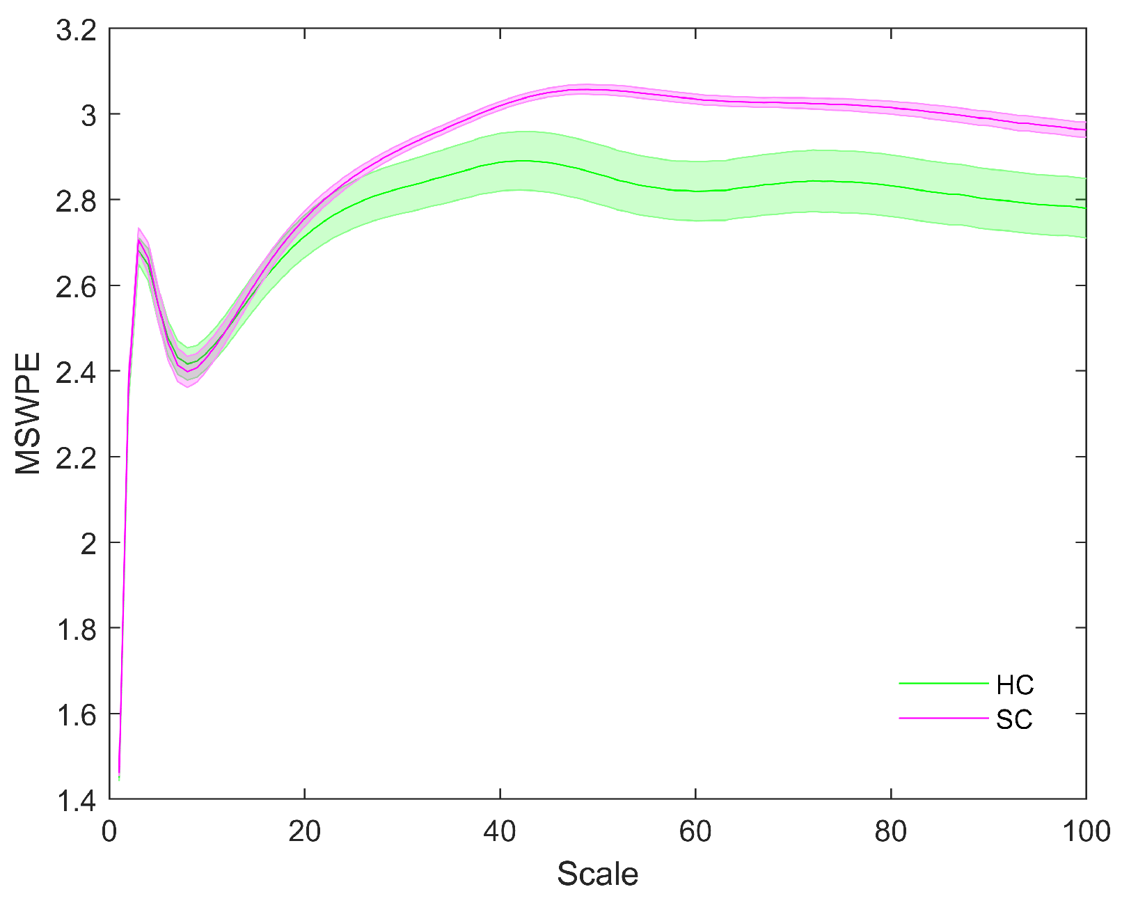
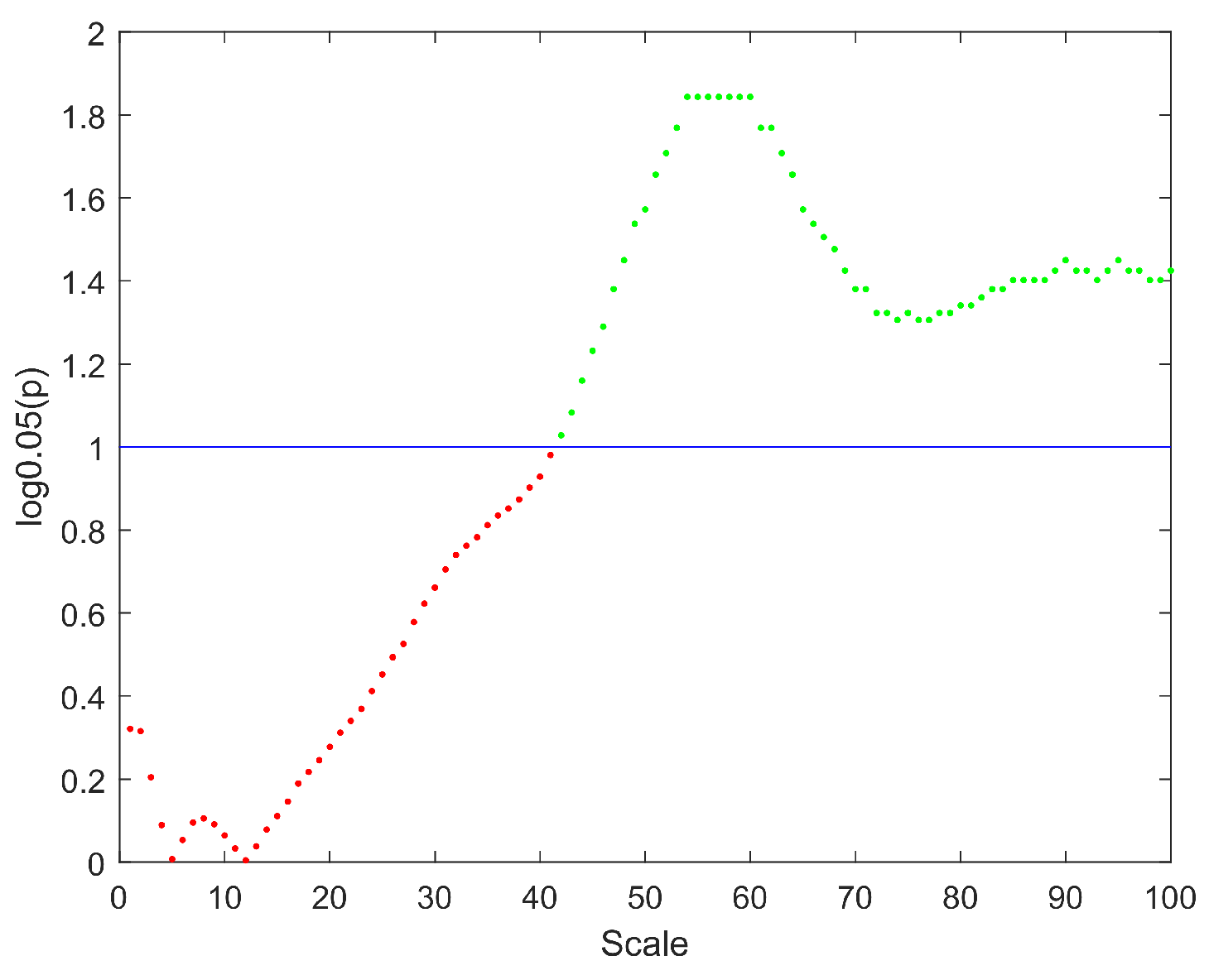
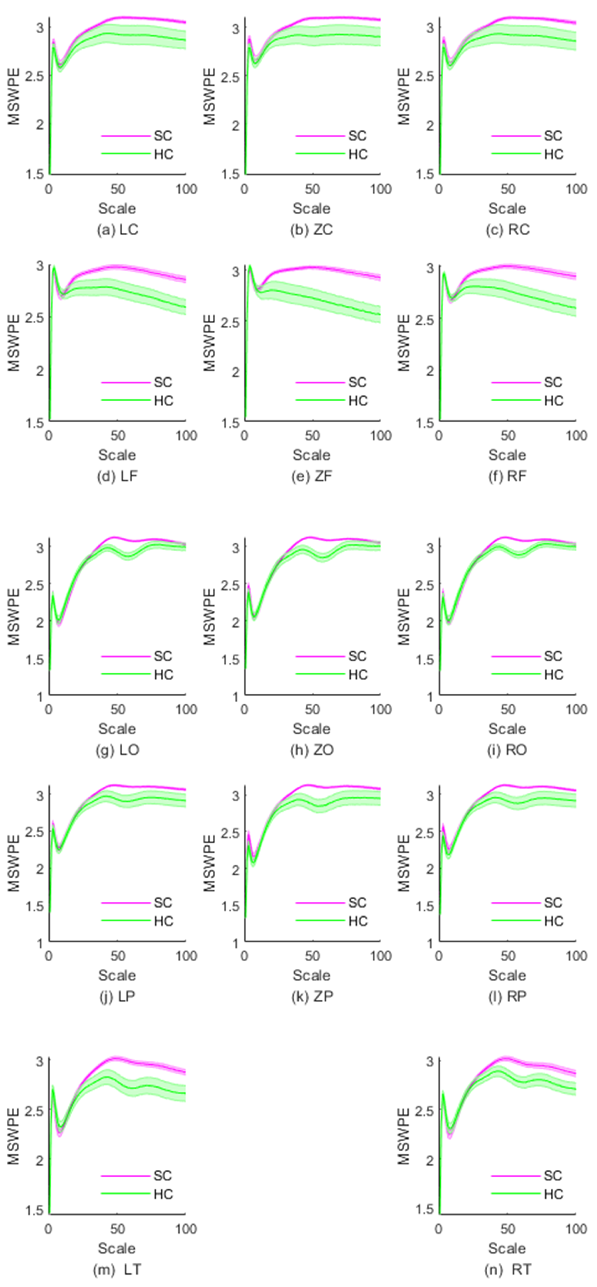
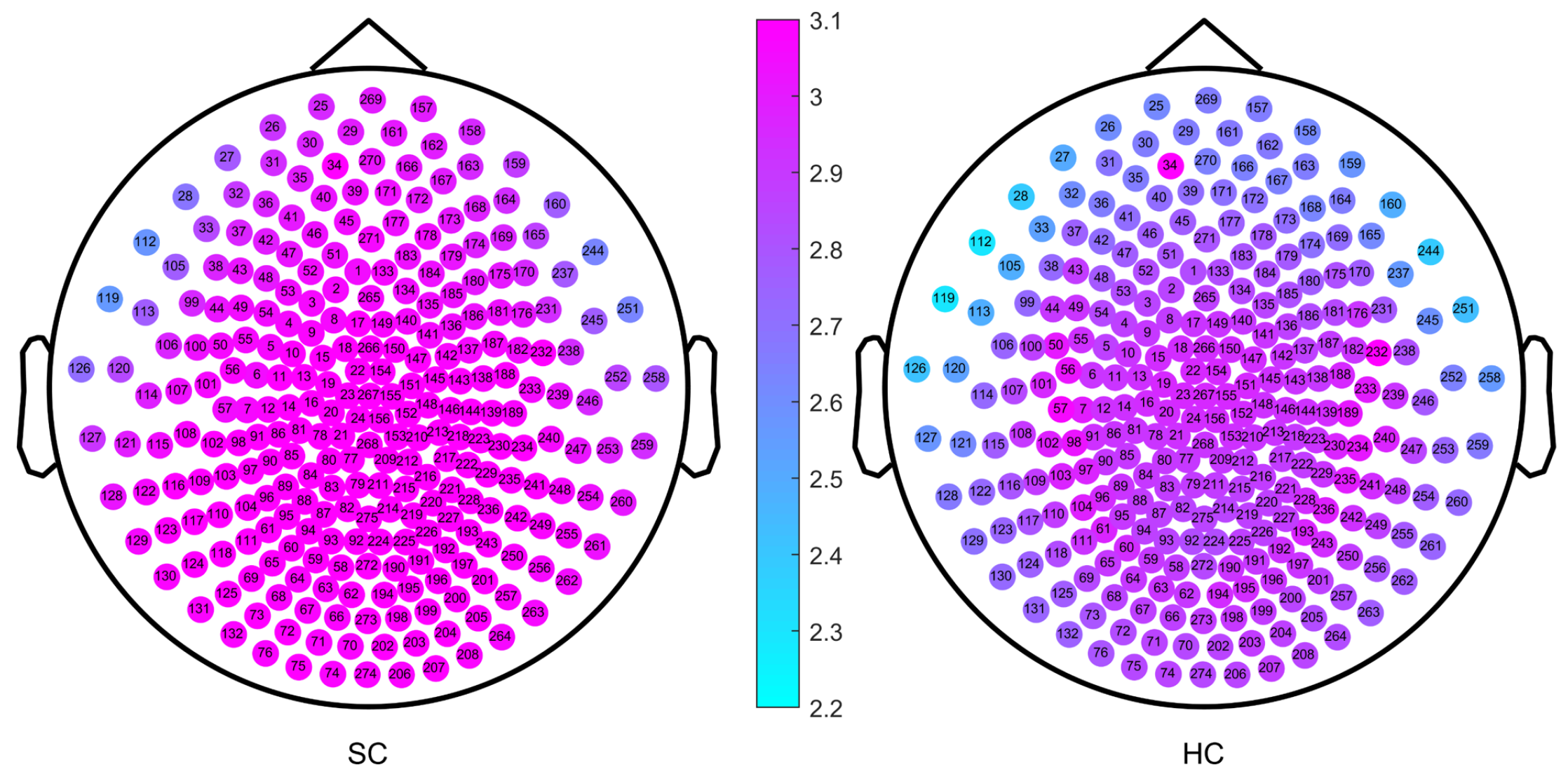
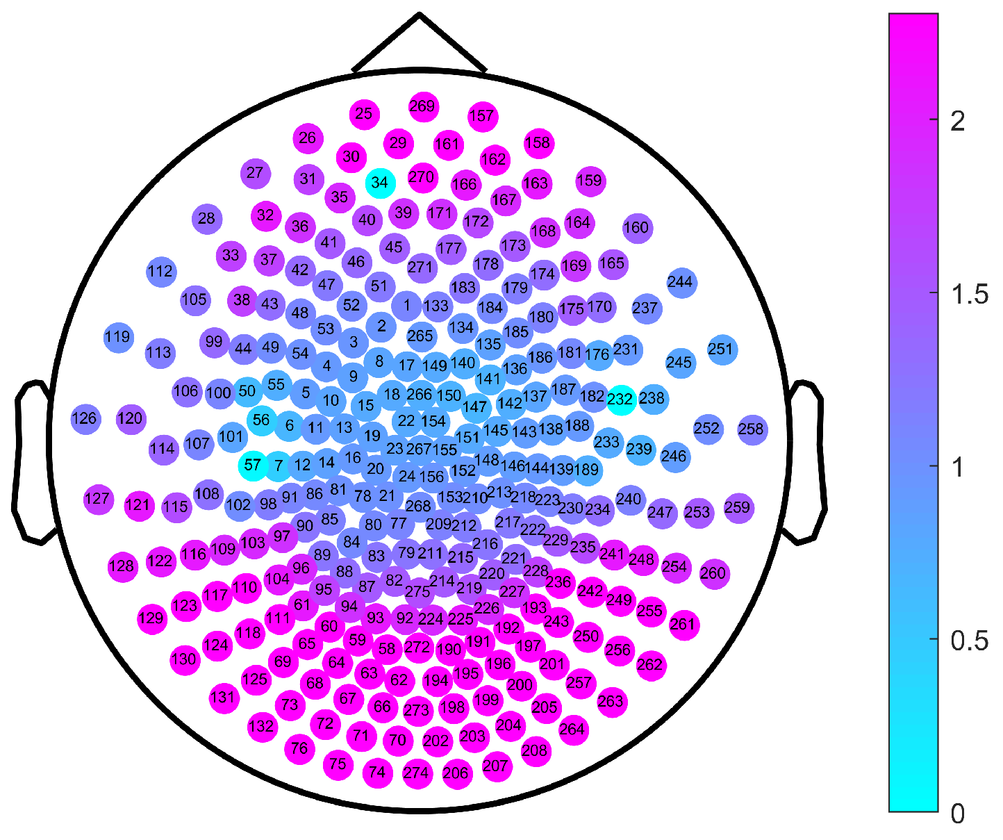
2. Results
3. Discussion
4. Materials and Methods
4.1. Participants
4.2. MEG Recording
4.3. Preprocessing of MEG Dataset
4.4. Multiscale Weighted Permutation Entropy
4.4.1. Coarse-Graining Process
4.4.2. Weighted Permutation Entropy
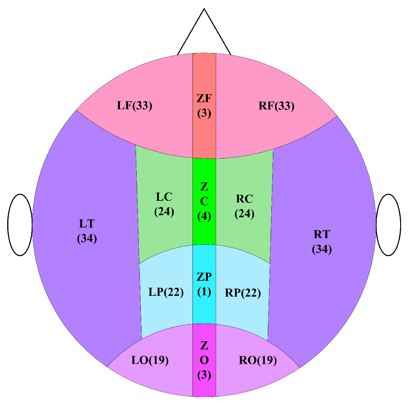
4.5. Division of Brain Regions
4.6. Statistical Analysis
5. Conclusions
Author Contributions
Funding
Institutional Review Board Statement
Informed Consent Statement
Data Availability Statement
Acknowledgments
Conflicts of Interest
Abbreviations
| MEG | Magnetoencephalogram |
| EEG | Electroencephalogram |
| fMRI | Functional magnetic resonance imaging |
| sMRI | Structural magnetic resonance imaging |
| PET | Positron emission tomography |
| CT | Computed tomography |
| LZ | Lempel-Ziv |
| PE | Permutation entropy |
| WPE | Weighted permutation entropy |
| MSE | Multiscale entropy |
| MSWPE | Multiscale weighted permutation entropy |
| FNN | False nearest neighbors |
| SC | Schizophrenia patients |
| HC | Healthy control |
| ECG | Electrocardiogram |
| EOG | Electrooculogram |
References
- World Health Organization Schizophrenia. January 2022. Available online: https://www.who.int/news-room/fact-sheets/detail/schizophrenia (accessed on 2 February 2022).
- Xu, T.; Stephane, M.; Parhi, K.K. Abnormal neural oscillations in schizophrenia assessed by spectral power ratio of MEG during word processing. IEEE Trans. Neural Syst. Rehabil. Eng. 2016, 24, 1148–1158. [Google Scholar] [CrossRef] [PubMed]
- Wang, M.; Huang, T.Z.; Fang, J.; Calhoun, V.D.; Wang, Y.P. Integration of imaging (epi) genomics data for the study of schizophrenia using group sparse joint nonnegative matrix factorization. IEEE/ACM Trans. Comput. Biol. Bioinform. 2019, 17, 1671–1681. [Google Scholar] [CrossRef] [PubMed]
- McCutcheon, R.A.; Marques, T.R.; Howes, O.D. Schizophrenia—An overview. JAMA Psychiatry 2020, 77, 201–210. [Google Scholar] [CrossRef] [PubMed]
- NIMH.Schizophrenia. Last Revised: May 2020. Available online: https://www.nimh.nih.gov/health/topics/schizophrenia/ (accessed on 2 February 2022).
- Müller, N. Inflammation in schizophrenia: Pathogenetic aspects and therapeutic considerations. Schizophr. Bull. 2018, 44, 973–982. [Google Scholar] [CrossRef] [PubMed] [Green Version]
- Millan, M.J.; Andrieux, A.; Bartzokis, G.; Cadenhead, K.; Dazzan, P.; Fusar-Poli, P.; Gallinat, J.; Giedd, J.; Grayson, D.R.; Heinrichs, M.; et al. Altering the course of schizophrenia: Progress and perspectives. Nat. Rev. Drug Discov. 2016, 15, 485–515. [Google Scholar] [CrossRef] [Green Version]
- Vita, A.; Barlati, S. Recovery from schizophrenia: Is it possible? Curr. Opin. Psychiatry 2018, 31, 246–255. [Google Scholar] [CrossRef]
- Edgar, J.C.; Guha, A.; Miller, G.A. Magnetoencephalography for Schizophrenia. Neuroimaging Clin. 2020, 30, 205–216. [Google Scholar] [CrossRef]
- Rojas, D.C. Review of schizophrenia research using MEG. In Magnetoencephalography: From Signals to Dynamic Cortical Networks; Springer Nature: Cham, Switzerland, 2019; pp. 1121–1146. [Google Scholar]
- Candelaria-Cook, F.T.; Schendel, M.E.; Ojeda, C.J.; Bustillo, J.R.; Stephen, J.M. Reduced parietal alpha power and psychotic symptoms: Test-retest reliability of resting-state magnetoencephalography in schizophrenia and healthy controls. Schizophr. Res. 2020, 215, 229–240. [Google Scholar] [CrossRef]
- Sauer, A.; Grent, T.; Jong, M.W.; Grube, M.; Singer, W.; Uhlhaas, P.J. A MEG Study of Visual Repetition Priming in Schizophrenia: Evidence for Impaired High-Frequency Oscillations and Event-Related Fields in Thalamo-Occipital Cortices. Front. Psychiatry 2020, 11, 561973. [Google Scholar] [CrossRef]
- Boutros, N.N.; Gjini, K.; Wang, F.; Bowyer, S.M. Evoked potentials investigations of deficit versus nondeficit schizophrenia: EEG-MEG preliminary data. Clin. EEG Neurosci. 2019, 50, 75–87. [Google Scholar] [CrossRef]
- Coffman, B.A.; Murphy, T.K.; Haas, G.; Olson, C.; Cho, R.; Ghuman, A.S.; Salisbury, D.F. Lateralized evoked responses in parietal cortex demonstrate visual short-term memory deficits in first-episode schizophrenia. J. Psychiatr. Res. 2020, 130, 292–299. [Google Scholar] [CrossRef] [PubMed]
- Alamian, G.; Hincapié, A.S.; Pascarella, A.; Thiery, T.; Combrisson, E.; Saive, A.L.; Martel, V.; Althukov, D.; Haesebaert, F.; Jerbi, K. Measuring alterations in oscillatory brain networks in schizophrenia with resting-state MEG: State-of-the-art and methodological challenges. Clin. Neurophysiol. 2017, 128, 1719–1736. [Google Scholar] [CrossRef]
- Roach, B.J.; D’Souza, D.C.; Ford, J.M.; Mathalon, D.H. Test-retest reliability of time-frequency measures of auditory steady-state responses in patients with schizophrenia and healthy controls. Neuroimage Clin. 2019, 23, 101878. [Google Scholar] [CrossRef] [PubMed]
- Braeutigam, S.; Dima, D.; Frangou, S.; James, A. Dissociable auditory mismatch response and connectivity patterns in adolescents with schizophrenia and adolescents with bipolar disorder with psychosis: A magnetoencephalography study. Schizophr. Res. 2018, 193, 313–318. [Google Scholar] [CrossRef] [PubMed]
- Zeev-Wolf, M.; Levy, J.; Jahshan, C.; Peled, A.; Levkovitz, Y.; Grinshpoon, A.; Goldstein, A. MEG resting-state oscillations and their relationship to clinical symptoms in schizophrenia. Neuroimage Clin. 2018, 20, 753–761. [Google Scholar] [CrossRef] [PubMed]
- Sklar, A.L.; Coffman, B.A.; Salisbury, D.F. Localization of Early-Stage Visual Processing Deficits at Schizophrenia Spectrum Illness Onset Using Magnetoencephalography. Schizophr. Bull. 2020, 46, 955–963. [Google Scholar] [CrossRef] [PubMed]
- Hamilton, A.; Northoff, G. Abnormal ERPs and Brain Dynamics Mediate Basic Self Disturbance in Schizophrenia: A Review of EEG and MEG Studies. Front. Psychiatry 2021, 12, 438. [Google Scholar] [CrossRef]
- Sanfratello, L.; Houck, J.M.; Calhoun, V.D. Relationship between MEG global dynamic functional network connectivity measures and symptoms in schizophrenia. Schizophr. Res. 2019, 209, 129–134. [Google Scholar] [CrossRef]
- Ohara, N.; Hirano, Y.; Oribe, N.; Tamura, S.; Nakamura, I.; Hirano, S.; Tsuchimoto, R.; Ueno, T.; Togao, O.; Hiwatashi, A.; et al. Neurophysiological Face Processing Deficits in Patients With Chronic Schizophrenia: An MEG Study. Front. Psychiatry 2020, 11, 554844. [Google Scholar] [CrossRef]
- Tang, L.; Yu, L.; Liu, F.; Xu, W. An integrated data characteristic testing scheme for complex time series data exploration. Int. J. Inf. Technol. Decis. Mak. 2013, 12, 491–521. [Google Scholar] [CrossRef]
- Zhao, Q.; Jiang, H.; Hu, B.; Li, Y.; Zhong, N.; Li, M.; Lin, W.; Liu, Q. Nonlinear dynamic complexity and sources of resting-state EEG in abstinent heroin addicts. IEEE Trans. Nanobiosci. 2017, 16, 349–355. [Google Scholar] [CrossRef] [PubMed]
- Ibáñez-Molina, A.J.; Lozano, V.; Soriano, M.; Aznarte, J.; Gómez-Ariza, C.J.; Bajo, M.T. EEG multiscale complexity in schizophrenia during picture naming. Front. Physiol. 2018, 9, 1213. [Google Scholar] [CrossRef] [PubMed] [Green Version]
- Tan, O.; Aydin, S.; HIZLI SAYAR, G.; Gürsoy, D. EEG complexity and frequency in chronic residual schizophrenia. Anatol. J. Psychiatry/Anadolu Psikiyatr. Derg. 2016, 17, 385–392. [Google Scholar] [CrossRef]
- Thilakvathi, B.; Shenbaga Devi, S.; Bhanu, K.; Malaippan, M. EEG signal complexity analysis for schizophrenia during rest and mental activity. Biomed. Res. India 2017, 28, 1–9. [Google Scholar]
- Fernández, A.; López-Ibor, M.I.; Turrero, A.; Santos, J.M.; Morón, M.D.; Hornero, R.; Gómez, C.; Méndez, M.A.; Ortiz, T.; López-Ibor, J.J. Lempel–Ziv complexity in schizophrenia: A MEG study. Clin. Neurophysiol. 2011, 122, 2227–2235. [Google Scholar] [CrossRef] [Green Version]
- Brookes, M.J.; Hall, E.L.; Robson, S.E.; Price, D.; Palaniyappan, L.; Liddle, E.B.; Liddle, P.F.; Robinson, S.E.; Morris, P.G. Complexity measures in magnetoencephalography: Measuring “disorder” in schizophrenia. PLoS ONE 2015, 10, e0120991. [Google Scholar] [CrossRef]
- Bandt, C.; Pompe, B. Permutation entropy: A natural complexity measure for time series. Phys. Rev. Lett. 2002, 88, 174102. [Google Scholar] [CrossRef]
- Bandt, C. Permutation Entropy and Order Patterns in Long Time Series. In Time Series Analysis and Forecasting; Springer: Berlin/Heidelberg, Germany, 2016; pp. 61–73. [Google Scholar]
- Yao, W.; Yao, W.; Yao, D.; Guo, D.; Wang, J. Shannon entropy and quantitative time irreversibility for different and even contradictory aspects of complex systems. Appl. Phys. Lett. 2020, 116, 014101. [Google Scholar] [CrossRef]
- Bai, Y.; Liang, Z.; Li, X. A permutation Lempel-Ziv complexity measure for EEG analysis. Biomed. Signal Process. Control 2015, 19, 102–114. [Google Scholar] [CrossRef]
- Rostaghi, M.; Azami, H. Dispersion entropy: A measure for time-series analysis. IEEE Signal Process. Lett. 2016, 23, 610–614. [Google Scholar] [CrossRef]
- Fadlallah, B.; Chen, B.; Keil, A.; Príncipe, J. Weighted-permutation entropy: A complexity measure for time series incorporating amplitude information. Phys. Rev. E 2013, 87, 022911. [Google Scholar] [CrossRef] [PubMed] [Green Version]
- Gao, X.; Chen, J.Y.; Zaki, M.J. Multiscale and multimodal analysis for computational biology. IEEE/ACM Trans. Comput. Biol. Bioinform. 2018, 15, 1951–1952. [Google Scholar] [CrossRef] [Green Version]
- Shi, J.; Zhao, J.; Liu, X.; Chen, L.; Li, T. Quantifying direct dependencies in biological networks by multiscale association analysis. IEEE/ACM Trans. Comput. Biol. Bioinform. 2018, 17, 449–458. [Google Scholar] [CrossRef] [PubMed]
- Costa, M.; Goldberger, A.L.; Peng, C.K. Multiscale entropy analysis of complex physiologic time series. Phys. Rev. Lett. 2002, 89, 068102. [Google Scholar] [CrossRef] [PubMed] [Green Version]
- Costa, M.; Goldberger, A.L.; Peng, C.K. Multiscale entropy analysis of biological signals. Phys. Rev. E 2005, 71, 021906. [Google Scholar] [CrossRef] [Green Version]
- Han, W.; Zhang, Z.; Tang, C.; Yan, Y.; Luo, E.; Xie, K. Power-Law Exponent Modulated Multiscale Entropy: A Complexity Measure Applied to Physiologic Time Series. IEEE Access 2020, 8, 112725–112734. [Google Scholar] [CrossRef]
- Yao, W.P.; Liu, T.B.; Wang, J. Multiscale permutation entropy analysis of electroencephalogram. Acta Phys. Sin. 2014, 63, 078704. [Google Scholar]
- Bai, D.; Yao, W.; Lv, Z.; Yan, W.; Wang, J. Multiscale multidimensional recurrence quantitative analysis for analysing MEG signals in patients with schizophrenia. Biomed. Signal Process. Control 2021, 68, 102586. [Google Scholar] [CrossRef]
- Li, R.; Wang, J. Interacting price model and fluctuation behavior analysis from Lempel–Ziv complexity and multi-scale weighted-permutation entropy. Phys. Lett. A 2016, 380, 117–129. [Google Scholar] [CrossRef]
- Chen, X.; Jin, N.D.; Zhao, A.; Gao, Z.K.; Zhai, L.S.; Sun, B. The experimental signals analysis for bubbly oil-in-water flow using multi-scale weighted-permutation entropy. Phys. A Stat. Mech. Its Appl. 2015, 417, 230–244. [Google Scholar] [CrossRef]
- Zheng, J.; Dong, Z.; Pan, H.; Ni, Q.; Liu, T.; Zhang, J. Composite multi-scale weighted permutation entropy and extreme learning machine based intelligent fault diagnosis for rolling bearing. Measurement 2019, 143, 69–80. [Google Scholar] [CrossRef]
- Kennel, M.B.; Brown, R.; Abarbanel, H.D. Determining embedding dimension for phase-space reconstruction using a geometrical construction. Phys. Rev. A 1992, 45, 3403–3411. [Google Scholar] [CrossRef] [PubMed] [Green Version]
- Kim, H.; Eykholt, R.; Salas, J. Nonlinear dynamics, delay times, and embedding windows. Phys. D Nonlinear Phenom. 1999, 127, 48–60. [Google Scholar] [CrossRef]
- Kang, S.S.; MacDonald III, A.W.; Chafee, M.V.; Im, C.H.; Bernat, E.M.; Davenport, N.D.; Sponheim, S.R. Abnormal cortical neural synchrony during working memory in schizophrenia. Clin. Neurophysiol. 2018, 129, 210–221. [Google Scholar] [CrossRef]
- Zhu, J.; Qian, Y.; Zhang, B.; Li, X.; Bai, Y.; Li, X.; Yu, Y. Abnormal synchronization of functional and structural networks in schizophrenia. Brain Imaging Behav. 2020, 14, 2232–2241. [Google Scholar] [CrossRef]
- Kelly, S.; Jahanshad, N.; Zalesky, A.; Kochunov, P.; Agartz, I.; Alloza, C.; Andreassen, O.; Arango, C.; Banaj, N.; Bouix, S.; et al. Widespread white matter microstructural differences in schizophrenia across 4322 individuals: Results from the ENIGMA Schizophrenia DTI Working Group. Mol. Psychiatry 2018, 23, 1261–1269. [Google Scholar] [CrossRef] [Green Version]
- Cetin-Karayumak, S.; Di Biase, M.A.; Chunga, N.; Reid, B.; Somes, N.; Lyall, A.E.; Kelly, S.; Solgun, B.; Pasternak, O.; Vangel, M.; et al. White matter abnormalities across the lifespan of schizophrenia: A harmonized multi-site diffusion MRI study. Mol. Psychiatry 2020, 25, 3208–3219. [Google Scholar] [CrossRef]
- Ivanov, P.C.; Amaral, L.A.N.; Goldberger, A.L.; Havlin, S.; Rosenblum, M.G.; Struzik, Z.R.; Stanley, H.E. Multifractality in human heartbeat dynamics. Nature 1999, 399, 461–465. [Google Scholar] [CrossRef] [Green Version]
- Akar, S.A.; Kara, S.; Latifoğlu, F.; Bilgiç, V. Analysis of the complexity measures in the EEG of schizophrenia patients. Int. J. Neural Syst. 2016, 26, 1650008. [Google Scholar] [CrossRef]
- Raghavendra, B.; Dutt, D.N.; Halahalli, H.N.; John, J.P. Complexity analysis of EEG in patients with schizophrenia using fractal dimension. Physiol. Meas. 2009, 30, 795–808. [Google Scholar] [CrossRef]
- Lee, S.H.; Choo, J.S.; Im, W.Y.; Chae, J.H. Nonlinear analysis of electroencephalogram in schizophrenia patients with persistent auditory hallucination. Psychiatry Investig. 2008, 5, 115–120. [Google Scholar] [CrossRef] [PubMed] [Green Version]
- Kay, S.R.; Fiszbein, A.; Opler, L.A. The positive and negative syndrome scale (PANSS) for schizophrenia. Schizophr. Bull. 1987, 13, 261–276. [Google Scholar] [CrossRef] [PubMed]
- Yao, W.P.; Yao, W.L.; Wang, J. Comparative analysis of the original and amplitude permutations. Phys. Lett. A 2022, 430, 127977. [Google Scholar] [CrossRef]

| Brain Region | Scale Intervals with Significant Differences | Minimum Value of p |
|---|---|---|
| LC | No significant difference | |
| ZC | No significant difference | |
| RC | No significant difference | |
| LF | [29, 100] | 0.001 |
| ZF | [24, 100] | |
| RF | [29, 100] | 0.001 |
| LO | [40, 72] | |
| ZO | [39, 72] | |
| RO | [40, 72] | |
| LP | [46, 64] | 0.016 |
| ZP | [41, 66] | 0.006 |
| RP | [44, 65] | 0.009 |
| LT | [41, 100] | 0.002 |
| RT | [44, 100] | 0.002 |
Publisher’s Note: MDPI stays neutral with regard to jurisdictional claims in published maps and institutional affiliations. |
© 2022 by the authors. Licensee MDPI, Basel, Switzerland. This article is an open access article distributed under the terms and conditions of the Creative Commons Attribution (CC BY) license (https://creativecommons.org/licenses/by/4.0/).
Share and Cite
Bai, D.; Yao, W.; Wang, S.; Wang, J. Multiscale Weighted Permutation Entropy Analysis of Schizophrenia Magnetoencephalograms. Entropy 2022, 24, 314. https://doi.org/10.3390/e24030314
Bai D, Yao W, Wang S, Wang J. Multiscale Weighted Permutation Entropy Analysis of Schizophrenia Magnetoencephalograms. Entropy. 2022; 24(3):314. https://doi.org/10.3390/e24030314
Chicago/Turabian StyleBai, Dengxuan, Wenpo Yao, Shuwang Wang, and Jun Wang. 2022. "Multiscale Weighted Permutation Entropy Analysis of Schizophrenia Magnetoencephalograms" Entropy 24, no. 3: 314. https://doi.org/10.3390/e24030314
APA StyleBai, D., Yao, W., Wang, S., & Wang, J. (2022). Multiscale Weighted Permutation Entropy Analysis of Schizophrenia Magnetoencephalograms. Entropy, 24(3), 314. https://doi.org/10.3390/e24030314